Continuous NMC Secure Against Permutations and Overwrites, with Applications to CCA Secure Commitments

Abstract

Non-Malleable Codes (NMC) were introduced by Dziembowski, Pietrzak and Wichs in ICS 2010 as a relaxation of error correcting codes and error detecting codes. Faust, Mukherjee, Nielsen, and Venturi in TCC 2014 introduced an even stronger notion of non-malleable codes called continuous non-malleable codes where security is achieved against continuous tampering of a single codeword without re-encoding.

We construct information theoretically secure CNMC resilient to bit permutations and overwrites, this is the first Continuous NMC constructed outside of the split-state model.

In this work we also study relations between the CNMC and parallel CCA commitments. We show that the CNMC can be used to bootstrap a Self-destruct parallel CCA bit commitment to a Self-destruct parallel CCA string commitment, where Self-destruct parallel CCA is a weak form of parallel CCA security. Then we can get rid of the Self-destruct limitation obtaining a parallel CCA commitment, requiring only one-way functions.

I. Damgård and M. Obremski—This work was supported by MPCPRO, ERC project nr. 669255.

T. Kazana—Supported by Polish National Science Centre (NCN) SONATA GRANT UMO-2014/13/D/ST6/03252.

L. Siniscalchi—This research received funding from: COST Action IC1306; “GNCS - INdAM”. The work of 5th author has been done in part while visiting Aarhus University, Denmark.

1 Introduction

In this paper, we study the interesting relationship between the notions of non-malleable codes and non-malleable commitments, and advance state of art for both of them. Before giving our results, we introduce the notions.

1.1 Introduction to Non-malleable Codes

Non-Malleable Codes (NMC) were introduced by Dziembowski, Pietrzak and Wichs [27] as a relaxation of error correcting codes and error detecting codes. An NMC takes a message m and encodes it as a possibly longer and randomized codeword $c \leftarrow {\mathsf {Enc}}(m)$. The adversary chooses and submits a tampering function $\mathsf {Tamper}$, that is applied to the code word to yield $c' = \mathsf {Tamper}(c)$. Applying the decoding algorithm yields a message $m' = \mathsf{{Dec}}(c')$. The security guarantee for an NMC now is that the decoded message $m'$ is either identical to the original message m or, in case of a decoding error, a message unrelated to m. Correspondingly, the adversary is given either $m'$ or a symbol “same” indicating that decoding was successful. Technically, we require that if $m' \ne m$, then $m'$ can be simulated using just the tampering function $\mathsf {Tamper}$, but without knowing anything about the tampered codeword $c'$.

It is generally impossible to give any meaningful guarantees if the tampering function is unrestricted (the tamper function could decode, and then encode a modified message). Therefore, the tampering function $\mathsf {Tamper}$ is always assumed to come from some class $\mathbb {T}$ of functions. An immediate example application of NM codes is for tamper resilient cryptography: if a secret key is stored in a hardware device, the adversary could try to tamper with the device and observe its behavior after the modification. But if the key is encoded with an NM code, the security guarantees immediately imply that either the tampering had no effect or the effect can be simulated without the device.

Continuous Non-Malleable Codes (CNMC). As mentioned in [37], non-malleable codes can provide protection against these kind of attacks if the device is allowed to freshly re-encode its state after each invocation to make sure that the tampering is applied to a fresh codeword at each step. After each execution the entire content of the memory is erased. While such perfect erasures may be feasible in some settings, they are rather problematic in the presence of tampering. Due to this reason, Faust et al. [28] introduced an even stronger notion of non-malleable codes called continuous non-malleable codes where security is achieved against continuous tampering of a single codeword without re-encoding. In this model the adversary can iteratively submit tampering functions $\mathsf {Tamper}_i$ and learn $m_i = \mathsf{{Dec}}(\mathsf {Tamper}_i(c))$. We call this the continuous tampering model. This stronger security notion is needed in many setting, for instance when using NMCs to make tamper resilient computations on von Neumann architectures [29].

Some additional restrictions are, however, necessary in the continuous tampering model. If the adversary was given an unlimited budget of tampering queries, then, given that the class of tampering functions is sufficiently expressive (e.g. it allows to overwrite single bits of the codeword), the adversary can efficiently learn the entire message just by observing whether tampering queries leave the codeword unmodified or lead to decoding errors, see e.g. [31].

To overcome this general issue, [28] assume a self-destruct mechanism which is triggered by decoding errors. In particular, once the decoder outputs a special symbol $\bot$ the device self-destructs and the adversary loses access to his tampering oracle. This model still allows an adversary many tamper attempts, as long as his attack remains covert. Jafargholi and Wichs [37] considered four variants of continuous non-malleable codes depending on

• Whether tampering is persistent in the sense that the tampering is always applied to the current version of the tampered codeword, and all previous versions of the codeword are lost. The alternative definition considers non-persistent tampering where the device resets after each tampering, and the tampering always occurs on the original codeword.

• Whether tampering to an invalid codeword (i.e., when the decoder outputs $\bot$) causes a “self-destruct” and the experiment stops and the attacker cannot gain any additional information, or alternatively whether the attacker can always continue to tamper and gain information.

A long line of research has tried to optimize the performance of NM codes with respect to the number of allowed tampering queries and the class of allowed tampering functions (see the related work section for details). In this paper we will be concerned with the case of CNMCs where there is no a priori bound on the number of queries. This model must include a self-destruct mechanism. Further we will be concerned with information theoretic NM codes where security holds for an unbounded adversary, and we will look at the single state model, where the tampering function is allowed to access the entire codeword. This is in contrast to the split-state model where the tamper function must consider disjoint parts of the codeword separately.

1.2 NMC- Our Result

We give a construction of a self-destruct, non-persistent continuous NMC (see Corollary 1 of Theorem 1) unconditionally secure against bit permutations composed with bit overwrites.

[5] gives a one time Non-Malleable Code resilient against bit permutations composed with bit-wise tampering. In [22] they construct a CNMC secure against bitwise tampering (but permutations are not allowed).

Unconditionally secure Continuous Non-Malleable Codes are notoriously hard to construct. Very little progress was made since CNMC were proposed in 2015:

• [22] authors construct a CNMC secure against bitwise tampering which is the variant of split-state model.

• [14] authors achieve a so-called many-many non-malleable code in the 2-split state model. Their construction achieves non-malleability as long as the number of rounds of tampering is at most $n^\gamma$ for some constant $\gamma < 1$, where n is the length of the codeword.

• [4] authors give the persistent continuous NMC construction for 2–split state.

• [3] gives Continuous NMC against 8–split state tampering (optimal number of states would be 3).

This makes our result the first known unconditionally secure construction of CNMC outside of split-state model.

1.3 NMC- Related Work

In [27] the authors construct an efficient code which is non-malleable with respect to bit-wise tampering, i.e., tampering functions that modify each bit of the codeword arbitrarily but independently of the value of the other bits of the codeword. Later works [2, 15, 17, 26, 42] provided stronger results by considering a model where the codeword is split into s parts called states, which can each be tampered arbitrarily but independently of the other states. explicit constructions were later given in [16, 30]. Other works considered tampering via permutations and perturbations [6], which are not captured in the split-state model. In [7] authors show how to construct efficient, unconditionally secure non-malleable codes for bounded output locality (i.e. when every bit of tampering output can depend on at most some $n^\delta$ bits of input for $\delta <1$).

The definition in [27] allows the adversary to be computationally unbounded. We call this an information theoretic NMC. Later works considered a notion of computational NMC where the adversary and tampering functions are restricted to efficient computations, see for instance [1, 8, 18, 46]. The definition in [27] allows the adversary to tamper the codeword only once. We call this one-shot tampering. Faust et al. [28] consider a stronger model where the adversary can iteratively submit tampering functions $\mathsf {Tamper}_i$ and learn $m_i = \mathsf{{Dec}}(\mathsf {Tamper}_i(c))$. We call this the continuous tampering model. This stronger security notion is needed in many setting, for instance when using NMCs to make tamper resilient computations on von Neumann architectures [29]. Some additional restrictions are, however, necessary in the continuous tampering model. If the adversary was given an unlimited budget of tampering queries, then, given that the class of tampering functions is sufficiently expressive (e.g. it allows to overwrite single bits of the codeword), the adversary can efficiently learn the entire message just by observing whether tampering queries leave the codeword unmodified or lead to decoding errors, see e.g. [31].

To overcome this general issue, [28] assume a self-destruct mechanism which is triggered by decoding errors. In particular, once the decoder outputs a special symbol $\bot$ the device self-destructs and the adversary loses access to his tampering oracle. This model still allows an adversary many tamper attempts, as long as his attack remains covert. Jafargholi and Wichs [37] provide a general study of when CNMCs can be built assuming a self-destruct mechanism.

Faust et al. [28] constructed a CNMC in the 2-state model which is secure against computationally bounded adversaries. It was shown in the same work that it is impossible to construct an information theoretic CNMC for the 2-state model.

Information-theoretic results for CNMC. In [22] authors construct a CNMC secure against bitwise tampering which is the simplest variant of split-state model. In [4] authors give the first information theoretic persistent continuous NMC construction for 2–split state. Finally in [3] authors give the first information theoretic construction of CNMC in 8–split state. Before [3] the only known result that achieves some sort of non-malleable codes secure against non-persistent continuous tampering was the result by Chattopadhyay, Goyal, and Li [14]. They achieve this by constructing a so-called many-many non-malleable code in the 2-split state model. Their construction achieves non-malleability as long as the number of rounds of tampering is at most $n^\gamma$ for some constant $\gamma < 1$, where n is the length of the codeword.

1.4 Application to Commitment Schemes

Commitment Schemes. The notion of commitment is perhaps the most fundamental concept in cryptographic protocol design. The idea is that a sender binds herself to a choice of a message m by exchanging some information with a receiver. The commitment should be hiding, i.e., the verifier does not learn the committed message. Later, the sender can choose to open the commitment, i.e., release more information allowing the receiver to determine m. The commitment should be binding, i.e., the sender cannot make the receiver output a message different from the one she had in mind at commit time.

The strongest possible security notion for commitment schemes is UC security, which intuitively asks that using the scheme is equivalent to giving m to a trusted party who will only release it on request from the committer. This is much stronger than simply asking for hiding and binding, e.g., we get security under general composition. But unfortunately, we know that UC security cannot be achieved without set-up assumptions. So a long line of research has been aimed at achieving weaker but meaningful security guarantees without set-up.

An important example of this is the notion of non-malleable (NM) commitments [24]. Here we consider an adversarial Man-in-the-middle (MiM), who on side receives a commitment from an honest sender to message m (the “left session”) and on the other side sends a commitment to an honest receiver (the“right session”), containing $m'$. The MiM wins if he succeeds in forming a new commitment on the right such that $m'$ has some non-trivial relation to m. The NM property does not follow from hiding and binding and is very important, for instance in making auctions where committed bid is fair, or towards implementing secure coin-flipping. Technically the NM property is captured by requiring a simulator that will simulate the left session without knowing m and still the MiM wins with essentially the same probability.

The strongest form of NM commitment security is concurrent NM commitments. Here, the MiM is allowed to start any number of left sessions and right sessions and can schedule them as he likes. One can also consider restricted versions of this, for instance a 1–1 NM commitment is secure if only 1 left and 1 right session is allowed. A restriction that we want to consider is self-destruct (SD) concurrent non-malleable commitment. In this version, once the MiM makes a invalid commitment in a right session, all commitment computed after that session are considered invalid and cannot be used to win the game. This notion is close in spirit to the one of the weak non-malleable commitments, which has been applied in multiple works.

An even stronger notion of commitment security is CCA security ([12]): we consider again a MiM, but he is now given an oracle that he can query on input a commitment from (one of) the right session(s), as long as it is not a copy of something from a left session. The requirement is that hiding holds for the left session(s), even in presence of the oracle. Intuitively, a CCA secure commitment is also NM secure, all other things being equal: if the MiM could break NM security and come up with a new commitment on the right side that is related to one from the left, he could submit it to the oracle in the CCA game and use the reply to break hiding on the left side. One restriction on CCA commitments that has been considered is parallel CCA security, where the MiM can ask only one query that may, however, contain an unbounded number of commitments. Another restriction is that of self-destruct (SD)-CCA, where the oracle stops working if the MiM submits an invalid commitment.

Parallel CCA Commitments from CNMC. In this second part we investigate possible applications our CNMC. In particular, we will show a bridge between (unconditionally secure) CNMC and (computational) cryptographic primitives secure in the concurrent setting.

For the stand-alone setting the result of [5] shows how to use a bit parallel CCA commitment¹ to construct a 1-1 string non-malleable commitment relying on stand-alone NM code. In particular, constructing string commitment from the corresponding 1-bit primitive, they first encode the input message with an NM code and then apply a 1-bit commitment scheme.

Following the same approach of [5] but using a CNMC (resilient to the same class of tampering functions of [5]) we are asking which flavor of non-malleability w.r.t. commitment we can achieve. In particular, is it enough to plug-in our CNMC in the construction of [5] to obtain a concurrent NM string commitment? The answer is only partially yes, due to the self-destruct limitation of CNMC. Indeed, a MiM adversary of NM commitments can compute multiple invalid commitments. Then, we show how to bypass this limitations requiring only OWFs.

In more details, we obtain a compiler that takes a CCA bit commitment and constructs an SD concurrent NM commitment. Due to the adaptiveness of our NM code we actually achieve a stronger security notion, namely a string SD-CCA commitment scheme. Furthermore we can relax the requirements on the CCA bit commitment: it just needs to be SD-CCA-secure instead of CCA-secure.

Summarizing, we show a compiler that on input a (non-tag based) SD-CCA bit commitment scheme and a continuous non-malleable code resilient against permutations and bit overwrites, outputs a (non-tag based) SD-CCA string commitment scheme. Our construction, like the one of [5], preserves the round complexity of the bit commitment scheme and does not require any additional assumption. Finally, we show that a SD-parallel CCA string commitment scheme can be upgraded to a parallel string commitment scheme without self-destruct, assuming only one-way functions. The construction is non-trivial (it requires very recent developed tecniques) and adds only two rounds of interaction.

Together with our compiler described above, this implies the first construction that exploit the CNMC property to obtain a parallel CCA commitment. Furthermore, parallel CCA commitment founds multiple applications like [10, 41]. Observe that parallel CCA commitment is not implied by parallel NM commitment (see [11]).

Previous Work on NMCs and NM Commitments. The literature presents works that exploit the properties of the non-malleable code to construct non-malleable commitments. Goyal et al. [35] use non-malleable codes in the split-state model to realize a 3-round one-one non-malleable commitment relying on one way permutations secure against a quasi-polynomial time adversary. Chandran et al. [13] show that block non-malleable codes with t blocks imply non-malleable commitments of $t-1$ rounds. As we discuss above, Agrawal et al. [5] showed that is possible to construct a one-one non-malleable commitment relying on a non-malleable code and a bounded parallel CCA bit commitment. However, no one before uses non-malleable codes to construct a parallel CCA commitment scheme. The aim of this second part is to build bridges between different notions of non-malleability, and to not construct a new NM commitment or a CCA commitment that are already available in literature. Indeed, there is a long line of research that tries to reduce the round complexity of NM commitment (e.g. [9, 19, 20, 24, 32, 33, 35, 36, 38, 39, 43, 45, 47,48,49]). Several constructions of CCA commitment are also available in literature (e.g. [12, 34, 40, 44]).

1.5 Technical Overview of Our CNMC Secure Against Permutations-and-Overwrites

Construction of Continuous Non-Malleable Code. Our code consists of an amalgamation of two different layers of encoding schemes.

The top layer is a Reed-Solomon code used here as a sharing scheme. We take a message m, append a random suffix and then encode it using Reed-Solomon to receive a codeword consisting of N blocks that may be seen as shares of $\lfloor \frac{N}{3} \rfloor$-out-of-N secret sharing scheme. The intuition behind this scheme is that the adversary needs to learn at least $\frac{N}{3}$ shares to learn anything about the initial message.

The bottom layer is using a Two-Split State Super Strong Non-Malleable Code (instantiated either by [4] or [42]). Each share $s_i$ from the above secret sharing scheme is converted into $(s_i||i)$ and then encoded using the two-split state code to get two shares $(L_i,R_i)$ (We also expect the bit-parity of $L_i$ to be 0 and the bit-parity of $R_i$ to be 1). The final code is $(L_1, R_1, ..., R_N, L_N)$.

To prove that the just described code is actually continuous non-malleable code, we first redefine the experiment in the definition of continuous codes. The new definition is obviously stronger, so it is sufficient to work with it. In the new definition, whenever an adversary tampers with a block $(L_i, R_i)$ with non-constant functions and succeeds in creating valid (from the point of view of Super Strong NMC decoder) output blocks $(L_i',R_i')$ (In particular, the parities of all $(L_i', R_i')$ must be correct), we will reveal blocks $(L_i, R_i)$ to the adversary.

As observed earlier, the adversary’s necessary task is to learn at least $\lfloor \frac{N}{3} \rfloor$ blocks of the underlying $s_i$ shares.

Since the adversary can only tamper bitwise and permute bits we can prove that if the adversary doesn’t know $\frac{N}{3}$ blocks and he tries to modify the codeword he will either get detected with probability exponentially close to 1, or he can attempt to learn some small amount information about the codeword (i.e. tamper with few blocks $L_i,R_i$ with non-constant function). However, using the bottom layer, we show that every attempt to learn even the smallest information about the codeword (i.e. by overwriting all but only few bits) yields some probability of detection which amplifies with amount of information adversary is trying to learn. We will therefore show that adversary can not (i.e. the probability is negligable) breach $\lfloor \frac{N}{3} \rfloor$ blocks threshold.

The argument consists of two main technical observations:

• If the adversary applies any non-constant functions f, g to single block $L_i,R_i$ then, due to combination of super strong nmc properties and parity requirements we have placed on $L_i,R_i$, adversary risks close to $\frac{1}{2}$ detection probability.

• If the adversary decides to mix bits between different blocks $(L_i, R_i)$ he has to risk violation of parity requirements on these blocks. This lemma is inspired by similar lemma for unary schemes from [6].

Using these ideas we can claim that if adversary tampers with k blocks using non-constant functions he also gets detected with a probability $1- p^{-k}$. The proof of this fact is more involved because we have to deal with minute cases. For example if we prove that mixing of bits will make the parity unpredictable for each block it still may happen that the events of error are correlated so not obviously amplify the error rate. Example 1. Assume adversary tampers only with $L_1$ and $L_2$, if he permutes bits in a way that output $L_1'$ contains first halfs of vectors $L_1, L_2$, $L_2'$ contains second halfs of $L_1, L_2$. Then parity of $L_1'$ is correct if and only if parity of $L_2'$ is correct. We handle this by picking only largest possible subset of independent parity checks. In this case we would focus only on parity of $L_1'$ and discard any other checks generated by $L_1, L_2, R_1, R_2$.

Example 2. Consider a tampering function which takes one bit from some blocks $(L_i,R_i)$ and permutes them to the last block $(L_N', R_N')$ while fixing all other $(L_i, R_i)$ to some constants. If $(L_N', R_N')$ has a correct parity and valid Super-Strong NMC decoding then we will reveal, to adversary, all blocks that’donated’ bits to $(L_N', R_N')$. Notice however that this will not reveal more bits then $|L_N|+|R_N|$ blocks.

Above examples illustrate how we bound number of blocks adversary can learn for each independent validity check he has to create.

1.6 Technical Overview of Our Self-destruct CCA Commitment and Parallel CCA Commitment

The Self-destruct CCA commitment scheme. We want to show that given a Self-destruct CCA bit commitment scheme (non-tag based), committing to each bit of the codeword individually, results in a Self-destruct CCA string commitment scheme. The security proof is based on the following high-level idea: if the adversary of the Self-destruct CCA string commitment is mauling, then, the attack on the commitment level can be “translated” into an attack on the non-malleable code. In other word, we can show an adversary $\mathcal {A}_{\mathsf {NMCode}}$ that breaks the security of the non-malleable code using the adversary $\mathcal {A}$ on the commitment level that distinguish a commitment of message $m_0$ from a commitment of message $m_1$. $\mathcal {A}_{\mathsf {NMCode}}$ will act as the sender in the left session with $\mathcal {A}$. Instead in the k-th right session (for $k=1,\dots , \mathtt{poly}(\lambda )$) $\mathcal {A}_{\mathsf {NMCode}}$ will act as a receiver of the string commitment. Then he needs to emulate the oracle $\mathcal {O}$ of the string commitment computing the following steps: (1) define a tamper function $f_k$ based on value v committed in the right session (note that he can obtain v querying the oracle of the bit commitment ²) (2) send back to $\mathcal {A}$ the decoding of $f_k(\mathsf{enc}_{m_b})$, where $\mathsf{enc}_{m_b}$ is an encoding of $m_b$ (received from the challenger of the non-malleable code game). At the end, $\mathcal {A}_{\mathsf {NMCode}}$ will output what $\mathcal {A}$ outputs. However we notice that the adversary that we described is not yet an adversary against the non-malleable code since the tamper functions can be dependent on what is committed on the left. We can demonstrate that the hiding of the Self-destruct CCA bit commitment ensures that the distribution of the tamper functions is computational independent from the message committed by the sender. Therefore the final adversary against the non-malleable code will simply commits to a random message on the left session. Finally, we crucially need that the non-malleable code is information theoretic secure since we have no guarantee that works in polynomial time.

Upgrade SD-PCCA Commitment Scheme to PCCA Commitment Scheme. At a very high level our PCCA string commitment scheme works as follows. The sender interacts with the receiver in order to compute a commitment $\tau$ of m using a Self-destruct PCCA string commitment. Furthermore, the receiver engages with the sender a protocol to allow the extraction of a trapdoor. We use the “trapdoor protocol” described in [20] where the trapdoor is represented by the knowledge of two signatures under a verification key sent by receiver in the 4th last round. In order to allow the extraction of the trapdoor, the receiver sends a signature of a randomly chosen message in the 3rd last round by the sender. Then, the sender executes a special witness-indistinguishable proof of knowledge (WIPoK) with the receiver in order to prove that he computed a valid commitment of m or that he knows a trapdoor.

Observe that if we use a 3-round WIPoK it is not clear how the proof of security will proceed. In particular, in the security proof there are some hybrids were we simulate the oracle of the parallel CCA commitment in polynomial time extracting the committed messages from the WIPoKs. Let us consider the hybrid were we switch the witness in one of the WIPoK. In the reduction to the WI we have to emulate the oracle of the parallel CCA commitments, since the reduction has to work in polynomial time. As we said, our hope to emulate the oracle is to extract the committed messages from the WIPoKs, however the extraction procedure rewinds also the challenger of the WI.

To overcome this problem we adopt the approach proposed in [20] relying on non-interactive primitives instead of 3-rounds WIPoK.

Therefore, similarly to [20], we construct this WIPoK relying on: instance-dependent trapdoor commitments (IDTC) and special honest-verifier zero knowledge (SHVZK).

In more details, let $({\mathsf {ls}}^1_{\mathsf {trap}},{\mathsf {ls}}^2_{\mathsf {trap}},{\mathsf {ls}}^3_{\mathsf {trap}},{\mathsf {ls}}^4_{\mathsf {trap}})$ be the transcript of a 4-round special HVZK delayed-input³ proof of knowledge (PoK). The transcript $({\mathsf {ls}}^1_{\mathsf {trap}},{\mathsf {ls}}^2_{\mathsf {trap}},{\mathsf {ls}}^3_{\mathsf {trap}},{\mathsf {ls}}^4_{\mathsf {trap}})$ is used to prove knowledge of two signatures of two different message w.r.t. a verification key sent by the receiver. The transcript $({\mathsf {ls}}^1_{\mathsf {trap}},{\mathsf {ls}}^2_{\mathsf {trap}},{\mathsf {ls}}^3_{\mathsf {trap}},{\mathsf {ls}}^4_{\mathsf {trap}})$ is used to prove the knowledge of the trapdoor.

At the 4th last round the sender sends an equivocal $\mathtt {com}$ obtained running IDTC. At last round the sender will equivocate $\mathtt {com}$ in order to send as opening $(\mathtt {dec}, {\mathsf {ls}}^2_{\mathsf {trap}})$. In the last round also ${\mathsf {ls}}^4_{\mathsf {trap}}$ is sent. The instance used for the IDTC is $\tau$, this means that the commitment $\mathtt {com}$ (computed using IDTC) can be opened to any value because $\tau$ is a well-formed commitment.

In the opening phase the sender sends the opening of the Self-destruct PCCA string commitment.

Note that the first two rounds of the “trapdoor protocol” can be run with the last two rounds of the Self-destruct commitment. Therefore the described construction has $t+2$ rounds (where t is the number of rounds of the Self-destruct PCCA string commitment).

Overview of the Security Proof. In the 1st experiment (the real game $RG_0$) the sender commits to $m_0$. We observe that due to the security of the signature scheme we can demonstrate that in the real game $\mathcal {A}$ is committing to a well-formed commitments in all parallel right sessions with non-negligible probability. Symmetrically there is the experiment $RG_1$ where the sender commits to $m_1$ and $\mathcal {A}$ is committing to a well-formed commitment in all parallel right sessions. Then we consider a hybrid game $\mathcal {H}_b^0$, for $b\in \{0,1\}$, where the sender commits to $m_b$ and the oracle is emulated extracting the committed values from the special WIPoK. Note that $\mathcal {H}_b^0$ is distributed statistically close to $RG_b$ until $\mathcal {A}$ receives the committed values, therefore we are ensured that we can extract the values committed in the right sessions. The 2nd hybrid game that we consider is $\mathcal {H}_b^1$ in which we switch the witness used to compute the transcript of the special WIPoK in the left sessions (i.e. we are using the trapdoor that is extracted by rewinding $\mathcal {A}$ in the left session). Using techniques that are similar to the one showed in [20] we are able to demonstrate that also in $\mathcal {H}_b^1$ we can extract the committed values in all parallel right sessions with non-negligible probability. Moreover, we can demonstrate that the distribution of the commitment values along with the view of $\mathcal {A}$ is indistinguishable between $\mathcal {H}_b^0$ and $\mathcal {H}_b^1$, for $b\in \{0,1\}$. Indeed, both in $\mathcal {H}_0^1$ and in $\mathcal {H}_1^1$ we are guaranteed that $\mathcal {A}$ is committing to a well-formed commitment in all parallel right sessions with non-negligible probability. Summing up, a detectable deviation from $\mathcal {H}_0^1$ and $\mathcal {H}_1^1$ implies a contradiction of the Self-destruct PCCA security of the underlining commitment. Finally we observe that the extraction procedure of the signatures does not interfere with the reductions since in the parallel right sessions the commitment phase made by $\mathcal {A}$ ends in the third last round. This observation concludes the high-level overview of the security proof.

2 Preliminaries

We denote the security parameter by $\lambda$ and use “||” as concatenation operator (i.e., if a and b are two strings then by a||b we denote the concatenation of a and b). We use the abbreviation ppt that stands for probabilistic polynomial time. We use $\mathtt{poly}(\cdot )$ to indicate a generic polynomial function and $\mathbb {N}$ to denote the set of positive integer.

A polynomial-time relation ${\mathsf {Rel}}$ (or polynomial relation, in short) is a subset of $\{0, 1\}^*\times \{0,1\}^*$ such that membership of (x, w) in ${\mathsf {Rel}}$ can be decided in time polynomial in |x|. For $(x,w)\in {\mathsf {Rel}}$, we call x the instance and w a witness for x. For a polynomial-time relation ${\mathsf {Rel}}$, we define the $\mathcal {N}\mathcal {P}$-language $L_{{\mathsf {Rel}}}$ as $L_{{\mathsf {Rel}}}=\{x|\exists w: (x, w)\in {\mathsf {Rel}}\}$.Analogously, unless otherwise specified, for an $\mathcal {N}\mathcal {P}$-language L we denote by ${\mathsf {Rel}}_\mathsf {L}$ the corresponding polynomial-time relation (that is, ${\mathsf {Rel}}_\mathsf {L}$ is such that $L=L_{{\mathsf {Rel}}_\mathsf {L}}$). We denote by $\hat{L}$ the language that includes both L and all well formed instances that do not have a witness. Moreover we require that membership in $\hat{L}$ can be tested in polynomial time. We implicitly assume that a PPT algorithm that is supposed to receive an instance in $\hat{L}$ will abort immediately if the instance does not belong to $\hat{L}$. Let A and B be two interactive probabilistic algorithms. We denote by $\langle A(\alpha ),B(\beta )\rangle (\gamma )$ the distribution of B’s output after running on private input $\beta$ with A using private input $\alpha$, both running on common input $\gamma$. Typically, one of the two algorithms receives $1^\lambda$ as input. A transcript of $\langle A(\alpha ),B(\beta )\rangle (\gamma )$ consists of the messages exchanged during an execution where A receives a private input $\alpha$, B receives a private input $\beta$ and both A and B receive a common input $\gamma$. Moreover, we will refer to the view of A (resp. B) as the messages it received during the execution of $\langle A(\alpha ),B(\beta )\rangle (\gamma )$, along with its randomness and its input. We say that a protocol (A, B) is public coin if B sends to A random bits only.

If $\mathcal{Z}$ is a set then $Z \leftarrow \mathcal{Z}$ will denote a random variable sampled uniformly from $\mathcal{Z}$. We start with some standard definitions and lemmas about the statistical distance. Recall that if X and $X'$ are random variables over the same set $\mathcal{X}$ then the statistical distance between X and $X'$ is denoted by $\varDelta (X;X')$, and defined as $\varDelta (X ; X') = \frac{1}{2} \sum _{x \in \mathcal{X}} |\Pr {X = x} - \Pr {X' = x}|$. If the variables X and $X'$ are such that $\varDelta (X ; X') \le \epsilon$ then we say that X is $\epsilon$-close to $X'$, and write $X \approx _{\epsilon } X'$. If $\mathcal{E},\mathcal{E}'$ are some events then by $\varDelta (X | \mathcal{E}\ ;\ X' | \mathcal{E}')$ we will denote the distance between variables $\widetilde{X}$ and $\widetilde{X}'$, distributed according to the conditional distributions $P_{X|\mathcal{E}}$ and $P_{X' | \mathcal{E}'}$.

If $U_{\mathcal{X}}$ is the uniform distribution over $\mathcal{X}$ then $d(X|\mathcal{E}) := \varDelta (X | \mathcal{E};U_\mathcal{X})$ is called statistical distance of X from uniform given the event $\mathcal{E}$. Moreover, if Y is independent from X then $d(X|Y) := \varDelta ((X,Y) ; (U_\mathcal{X},Y))$ is called statistical distance of X from uniform given the variable Y. More generally, if $\mathcal{E}$ is an event then $d(X | Y, \mathcal{E}) := \varDelta ((X,Y) | \mathcal{E}; (U_\mathcal{X},Y) | \mathcal{E})$. It is easy to see that d(X|Y) is equal to the average $\sum _{y} \Pr (Y = y) \cdot d(X | Y = y) = \mathbb {E}_y (d(X | Y = y))$.

Definition 1

((Average-) Min-Entropy). Let X have finite support $\mathcal{X}$. The min-entropy ${\mathbf {H}_{\infty }}(X)$ of X is defined by

$$\begin{aligned} {\mathbf {H}_{\infty }}(X) = - \log \max _{x \in \mathcal{X}} \Pr (X = x). \end{aligned}$$

For an event $\mathcal{E}$, the conditional min-entropy ${\mathbf {H}_{\infty }}(X | \mathcal{E})$ of X given $\mathcal{E}$ is defined by

$$\begin{aligned} {\mathbf {H}_{\infty }}(X | \mathcal{E}) = - \log \max _{x \in \mathcal{X}} \Pr (X = x | \mathcal{E}). \end{aligned}$$

For an event $\mathcal{E}$ and a random variable Y with finite support $\mathcal{Y}$, the average min-entropy ${\widetilde{\mathbf {H}}_{\infty }}(X | Y, \mathcal{E})$ of X given Y and $\mathcal{E}$ is defined by

$$\begin{aligned} {\widetilde{\mathbf {H}}_{\infty }}(X | Y, \mathcal{E}) = - \log \mathbb {E}_{y} \max _{x \in \mathcal{X}} \Pr (X = x | Y = y, \mathcal{E}). \end{aligned}$$

Randomness extractors will be the workhorses of our non-malleable code constructions.

Definition 2

(Flexible Two-Source Extractors). A function $\mathsf {Ext}: \mathcal{X}_1 \times \mathcal{X}_2 \rightarrow \mathcal{Z}$ is called a flexible $(\epsilon ,\delta )$-two-source extractor, if it holds for all tuples $((X_1,Y_1),(X_2.Y_2))$ for which $(X_1,Y_1)$ is independent of $(X_2,Y_2)$ and ${\widetilde{\mathbf {H}}_{\infty }}(X_1 | Y_1) + {\widetilde{\mathbf {H}}_{\infty }}(X_2 | Y_2) \ge \log (|\mathcal{X}|) + \log (|\mathcal{Y}|) - \delta$ that

$$\begin{aligned} d(\mathsf {Ext}(X_1,X_2) | Y_1,Y_2) \le \epsilon . \end{aligned}$$

A well known example of a flexible two-source extractor is the Hadamard extractor or inner-product-extractor.

Lemma 1

(Hadamard Extractor [2]). The function $\mathsf {Ext}: \mathbb {F}_q^n \times \mathbb {F}_q^n \rightarrow \mathbb {F}_q$ given by $\mathsf {Ext}(x,y) = \langle x,y \rangle$ is a flexible $(\epsilon ,\delta )$ extractor for $\delta \le (n-1)\log (q) - 2 \log (1 / \epsilon )$.

Lemma 2

(Entropy-preservation of inner-product for correlated distributions). Let X be random variable over $\mathcal{X}^l$, let C be random variable such that for every c we have ${\mathbf {H}_{\infty }}(X|C=c)\ge l\cdot \log |\mathcal{X}| - d$, where $d < \log |\mathcal{X}|$. Then for any non-zero $v\in \mathcal{X}^l$

$$\begin{aligned} {\mathbf {H}_{\infty }}(\langle X,v \rangle _{\mathcal{X}}\; | \;C=c)\ge \log |\mathcal{X}| -d \end{aligned}$$

for every c in $\mathsf {supp} (C)$.

We will now assemble a few basic technical lemmata that we will need for our proofs.

Lemma 3

(Bayes’ rule for statistical distance [26]). Let $(X,Y) \in \mathcal{X}\times \mathcal{Y}$ be a random variables, such that $d(X|Y) \le \epsilon$. Then for every $x \in \mathcal{X}$ we have

$$\begin{aligned} \varDelta (Y | X = x \ ; \ Y ) \le 2 |\mathcal{X}| \epsilon . \end{aligned}$$

Also if $\mathcal{A}$ is a random event such that $d(X|Y,\mathcal{A}) \le \epsilon$, we have:

$$\begin{aligned} \varDelta (Y | X = x, \mathcal{A}\ ; \ Y| \mathcal{A}) \le 2 |\mathcal{X}| \epsilon . \end{aligned}$$

Lemma 4

([25]). Let X, T be any arbitrarily correlated random variables and let $\mathcal{E}$ be random event then

$$\begin{aligned} {\widetilde{\mathbf {H}}_{\infty }}(X| T, \mathcal{E}) \ge {\widetilde{\mathbf {H}}_{\infty }}(X | T)- \log \frac{1}{\Pr (\mathcal{E})}. \end{aligned}$$

In the Appendix A the reader can find a series of standard definitions used in the rest of the paper.

2.1 Definitions Related to Non-Malleable Codes

Definition 3

(Coding Schemes). A coding scheme is a pair $({\mathsf {Enc}},\mathsf{{Dec}})$, where ${\mathsf {Enc}}: \mathcal{M}\rightarrow \mathcal{C}$ is a randomized function and $\mathsf{{Dec}}: \mathcal{C}\rightarrow \mathcal{M}\cup \{ \bot \}$ is a deterministic function, such that it holds for all $M \in \mathcal{M}$ that $\mathsf{{Dec}}({\mathsf {Enc}}(M)) = M$.

Definition 4

(Two-State Code). A coding scheme $({\mathsf {Enc}},\mathsf{{Dec}})$ where the counterdomain of ${\mathsf {Enc}}$ has the form $\mathcal{C}= \{0,1\}^k \times \{0,1\}^k$ is called a two-state code.

Definition 5

(Paritied Two-State Code). Let $({\mathsf {Enc}},\mathsf{{Dec}})$ (where ${\mathsf {Enc}}: \mathcal{M}\rightarrow \mathcal{C}= \mathcal{C}_1\times \mathcal{C}_2 = \{0,1\}^k \times \{0,1\}^k$) be a two-state code. Now let ${\mathsf {Enc}}^{par} : \mathcal{M}\rightarrow \mathcal{C}$ be a randomized function restricted to a condition that $parity({\mathsf {Enc}}(m)_1) = 0$ and $parity({\mathsf {Enc}}(m)_2) = 1$, where parity is a function calculating the parity of number of ones in a given vector (i.e. $parity(0101011) = 0$ and $parity(011111) = 1$).

More formally, the procedure computing ${\mathsf {Enc}}^{par}(m)$ can be described as follows: we run in a loop the encoding procudure $(c_1,c_2) \leftarrow {\mathsf {Enc}}(m)$ until $parity(c_1) = 0$ and $parity(c_2) = 1$.

Similarily, let $\mathsf{{Dec}}^{par}: \mathcal{C}\rightarrow \mathcal{M}\cup \{ \bot \}$ be defined as follows: for $c = (c_1, c_2) \in \mathcal{C}$, if $parity(c_1) \ne 0$ or $parity(c_2) \ne 1$ then $\mathsf{{Dec}}^{par}(c) := \bot$, otherwise $\mathsf{{Dec}}^{par}(c) := \mathsf{{Dec}}(c)$.

Now, the coding scheme $({\mathsf {Enc}}^{par}, \mathsf{{Dec}}^{par})$ is called a paritied two-state code.

We will now define the continuous tampering experiment. Our definition is a weaker version of [37]: instead of Super Strong Tampering experiment we will use the standard tamper experiment from [27].

Definition 6

((Continuous-) Tampering Experiment). We will define continuous non-persistent self-destruct non-malleable codes using [4] experiment, which is equivalent to original [27] experiment. Fix a coding scheme $({\mathsf {Enc}},\mathsf{{Dec}})$ with message space $\mathcal{M}$ and codeword space $\mathcal{C}$. Also fix a family of functions $\mathcal{F}: \mathcal{C}\rightarrow \mathcal{C}$. Let $\mathcal{D}=\{\mathcal{D}^f_{C}\}_{f\in \mathcal{F}, C \in \mathcal{C}}$ be some family of distributions over $\{0,1\}$, indexed by tampering function f and a codeword C. We will first define the tampering oracle $\mathsf {Tamper}^{\mathsf {state}}_{C,\mathcal{D}}(f)$, for which initially $\mathsf {state} = \mathtt {alive}$. For a tampering function $f \in \mathcal{F}$ and a codeword $C \in \mathcal{C}$ define the tampering oracle by

Fix a tampering adversary $\mathcal{A}$ and a codeword $C \in \mathcal{C}$. We define the continuous tampering experiment $\mathsf {CT}_{C,\mathcal{D}}(\mathcal{A})$ by

Definition 7

Let $({\mathsf {Enc}},\mathsf{{Dec}})$ be a coding scheme and $\mathsf {CT}$ be its corresponding continuous tampering experiment for a class $\mathcal{F}$ of tampering functions. We say that $({\mathsf {Enc}},\mathsf{{Dec}})$ is an $\epsilon$-secure continuously non-malleable code against $\mathcal{F}$, if there exists a family of distributions $\mathcal{D}=\{\mathcal{D}^f_{C}\}_{f\in \mathcal{F}, C \in \mathcal{C}}$ over $\{0,1\}$ such that for all tampering adversaries $\mathcal{A}$ and all pairs of messages $M_0,M_1 \in \mathcal{M}$ that

$$\begin{aligned} \mathsf {CT}_{C_0,\mathcal{D}}(\mathcal{A}) \approx _{\epsilon } \mathsf {CT}_{C_1,\mathcal{D}}(\mathcal{A}), \end{aligned}$$

where $C_0 \leftarrow {\mathsf {Enc}}(M_0)$ and $C_1 \leftarrow {\mathsf {Enc}}(M_1)$.

3 Continuous Non-Malleable Code Against Permutations-With-Overwrites

In this section we define a coding scheme $({\mathsf {Enc}}_c, \mathsf{{Dec}}_c)$ and prove it is a continuous non-malleable code against a class $\mathsf {PermOver}$ of permutations-with-overwrites (the actual definition will follow).

3.1 Coding Scheme

Let $\mathcal{M}= \{0,1\}^n$ and $\mathcal{C}= \mathcal{C}_1 \times \dots \times \mathcal{C}_N$, where each $\mathcal{C}_i = \{0,1\}^{k_1} \times \{0,1\}^{k_1}$. Let also $({\mathsf {Enc}}_2, \mathsf{{Dec}}_2)$ denote a two-state code (actually we need a two-state strong non-malleable code here, however the specific instantiation will be given later) and $h_N$ denote a $\lfloor N/3 \rfloor$-out-of-N secret sharing scheme (again, the specific instantiation will be given later). Now we are ready to introduce the (randomized) function (procedure) ${\mathsf {Enc}}_c: \mathcal{M}\rightarrow \mathcal{C}$:

For $m\in \mathcal{M}$ and a random $r \in \{0,1\}^n$, let $(d_1, \dots , d_N) \leftarrow h_N(m||r)$ where $(d_1, \dots , d_N) \in (\{0,1\}^{k_2})^N$ are shares for (m||r). Now, for each $d_i$ let $(L_i, R_i) \leftarrow {\mathsf {Enc}}_2^{par}(d_i || i)$.

Finally, we state $c_i \leftarrow (L_i, R_i)$ and ${\mathsf {Enc}}_s (m)$ outputs $(c_1, \dots , c_N)$.

The definition of $\mathsf{{Dec}}_c$ is simple and straightforward (forced by the definition of a coding scheme).

Remark 1

The above construction is not tight for a given message length n since it also depends on the choice of parameters $(N, k_1, k_2)$ and the specific definitions of both: the two-state code $({\mathsf {Enc}}_2, \mathsf{{Dec}}_2)$ and the secret sharing scheme $h_N$. However, before we pick adequate parameters and schemes, we need one definition more:

Definition 8

We call a two-split code $({\mathsf {Enc}}_2, \mathsf{{Dec}}_2)$ $\epsilon$-admissible if the scheme $({\mathsf {Enc}}_2^{par},\mathsf{{Dec}}_2^{par})$ fulfills the following requirements:

• 1. [Canonical encoding procedure:] ${\mathsf {Enc}}_2^{par}(m)$ is uniform in $\{c : \mathsf{{Dec}}_2^{par}(c)=m \}$.

• 2. [Detection of close to bijective tampering:] For any message m, if ${\mathsf {Enc}}_2^{par}(m)=(X,Y)$ then for any functions $f,g :\{0,1\}^{k_1} \rightarrow \{0,1\}^{k_1}$ such that ${\mathbf {H}_{\infty }}(f(X)),{\mathbf {H}_{\infty }}(g(Y)) \ge 2/3 \cdot k_1-1$ and (for any x or y) $f(x)\ne x$ or $g(y)\ne y$ it holds:

  $$\begin{aligned} \Pr (\mathsf{{Dec}}_2^{par}(f(X),g(Y))=\bot )\ge 1- \epsilon . \end{aligned}$$

• 3. [Detection of complete overwrite of one part:] For any constant $c\in \{0,1\}^{k_1}$, and any uniform $X, Y \in \{0,1\}^{k_1}$, such that parity of X is 0 and parity of Y is 1 we get,

  $$\begin{aligned} \Pr (\mathsf{{Dec}}_2(X,c)=\bot )\ge 1-\epsilon , \\ \Pr (\mathsf{{Dec}}_2(c,Y)=\bot )\ge 1-\epsilon \end{aligned}$$

• 4. [Leakage resilient storage:] For any message m, if ${\mathsf {Enc}}_2^{par}(m)=(X,Y)$ then for any functions $f,g :\{0,1\}^{k_1} \rightarrow \{0,1\}^{k_1}$ such that ${\widetilde{\mathbf {H}}_{\infty }}(X|f(X)) \ge 1/3 \cdot k_1$ and ${\widetilde{\mathbf {H}}_{\infty }}(Y|f(Y)) \ge 1/3 \cdot k_1$ we get

  $$\begin{aligned} \varDelta \left[ \left( f(X),Y \right) ; \left( f(U_0),U_1 \right) \right] \le \epsilon \ ,\\ \varDelta \left[ \left( X,g(Y) \right) ; \left( U_0,g(U_1) \right) \right] \le \epsilon \ , \end{aligned}$$

  where $U_0,U_1$ are independent uniformly distributed over $\{0,1\}^{k_1}$, such that parity of $U_i$ is equal i.

In the full version of the paper [23], we discuss possible instantiations (for an appropriate $\epsilon _c$) of Definition 8:

• with [4]: ${{\mathsf {Enc}}_{\mathsf {AKO}}}: \{0,1\}^m \rightarrow \left( \{0,1\}^{O(m^6)}\right) ^2$ is $2^{-O(m)}-$ admissible,

• with [42]:${{\mathsf {Enc}}_{\mathsf {Li}}}: \{0,1\}^m \rightarrow \left( \{0,1\}^{O(m\cdot \log m)}\right) ^2$ is $2^{-O(m)}-$ admissible.

(Of course the second code of the above gives better parameters. However we argue for both above statements.)

Through the rest of the paper we always refer to the second of the above specific two-state code and the specific error probability when notation $({\mathsf {Enc}}_2, \mathsf{{Dec}}_2)$ and $\epsilon _c$ is used.

3.2 Definition of the Class of Tampering Functions

Here we define the class $\mathsf {PermOver}$ of tampering functions. Through this paper functions from this class $\mathsf {PermOver}$ are called permutations-with-overwrites.

Let us consider a set $\{0,1\}^q$ of vectors of q bits (q-vectors, for short). Now, let denote $\varPi _q$ the class of permutations of bits of q-vectors. Denote also $O_q$ the class of functions $f : \{0,1\}^q \rightarrow \{0,1\}^q$, such that:

for all i, either $f(x)_i = x_i$ or $f(x)_i = b_i$ for a fixed $b_i$.

Loosely speaking: any function from $O_q$, independently for each bit, either leaves it unchanged or sets it into a fixed value (i.e. overwrites it).

Now we simply define the class $\mathsf {PermOver}_q = O_q \circ \varPi _q$. For our application we will equate $\mathcal{C}= (\{0,1\}^{k_1} \times \{0,1\}^{k_1})^N$ with $\{0,1\}^{2k_1N}$ and consider $\mathsf {PermOver}= \mathsf {PermOver}_{2k_1N}$ as a tampering class for $\mathcal{C}$.

The above description of course finishes the definition of our class of tampering functions, however we want a few further related definitions.

Related definitions. Let us fix a tampering function $t \in \mathsf {PermOver}$. As mentioned above we will think of t as a function from $\mathcal{C}_1 \times \dots \times \mathcal{C}_N$ to $\mathcal{C}_1 \times \dots \times \mathcal{C}_N$. Now, for each $i \in \{1, \dots , N\}$ we say that t either leaves or overwrites or modifies the i-th block. These phrases stand for the following:

If $t(c)_i = c_i$ then t leaves the i-th block. If $t(c)_i = a$ for some a independent of c then t overwrites the i-th block. Finally, if none of the previous occurs, then we say that t modifies the i-th block.

If t overwrites i-th block, two cases are possible. Either $c_i$ is independent of f(c) or some bits of $c_i$ are moved to some modified blocks. In the first case we say that t strong-overwrites i-th block and in the second case, it weak-overwrites.

Touched blocks are blocks either modified or weak-overwritten. In that case we say that t touches these blocks.

For a function $t\in \mathsf {PermOver}$ and a codeword $c\in \mathcal{C}$ we denote touch(t, c) the set of all touched blocks and its indices, more formally: $touch(t,c) = \{ (c_i, i) |$t$\text { touches } c_i \}$.

Example. The above definitions may look a little bit obscure at first sight, so – to make things clearer – we give an example.

Let $N = 4$ and each $\mathcal{C}_i = \{0,1\}^6$. Now let us consider:

$$\begin{aligned} t&\Big ( (b_1^1, b_2^1, b_3^1, b_4^1, b_5^1, b_6^1), (b_1^2, b_2^2, b_3^2, b_4^2, b_5^2, b_6^2), (b_1^3, b_2^3, b_3^3, b_4^3, b_5^3, b_6^3), (b_1^4, b_2^4, b_3^4, b_4^4, b_5^4, b_6^4) \Big ) = \\&\Big ( (0,0,0,1,1,1), (b_1^2, b_2^2, b_3^2, b_4^2, b_5^2, b_6^2), (0,1,0,1,0,1), (0, b_5^1, b_4^4, 1, b_2^4, b_1^1) \Big ). \end{aligned}$$

Obviously $t\in \mathsf {PermOver}$ and we have that: t leaves the second block, overwrites the first and the 3-rd block and modifies the 4-th block. The first block is weak-overwritten (because the 5-th block gets one bit from the first block) and the 3-rd block is strongly overwritten. Function t touches the blocks of the indices 1 and 4 so, for exemplary

$$c = ((0,0,1,1,0,0),(0,0,1,1,1,1),(1,1,1,1,0,0),(1,0,0,0,0,1)),$$

we have:

$$ touch(t,c) = \{ \big ((0,0,1,1,0,0),1\big ), \big ((1,0,0,0,0,1),4\big ) \} .$$

3.3 Statement and Proof

The main statements for the whole Sect. 3 are the following:

Theorem 1

The coding scheme $({\mathsf {Enc}}_c, \mathsf{{Dec}}_c)$ is an $(\alpha + 2 \epsilon _c)^{\lfloor N/3 \rfloor }$-secure continuous non-malleable code against $\mathsf {PermOver}$ for $\alpha = (0.5)^{\frac{1}{8\cdot k_1}}$.

Corollary 1

Instantiation for the above code with $(N, k_2, k_1) =$

$(6 \lceil n^{2/3} \rceil , \lceil n^{1/3} \rceil , c \lceil n^{1/3} \rceil \log {\lceil n^{1/3} \rceil })$, with $({\mathsf {Enc}}_2, \mathsf{{Dec}}_2) = ({{\mathsf {Enc}}_{\mathsf {Li}}},{\mathsf{{Dec}}_{\mathsf {Li}}})$ (see the end of Sect. 3.1) and $h_N = RS_N$ (see Appendix B) gives us a continuous non-malleable code against $\mathsf {PermOver}$ such that:

• the code rate is $O(\log n)$, and

• the error rate is $O(2^{-O(n^{1/3})})$.

Proof

The message length is n and the codeword length is $N \cdot 2 \cdot k_1 \approx 6 n^{2/3} \cdot 2 \cdot c n^{1/3} \frac{1}{3} \log n = 4 c n \log n$, so the code rate is approximately $4 c \log n = O(\log n)$. (Remark: c is a constant from ${{\mathsf {Enc}}_{\mathsf {Li}}}$ rate.) The error rate is:

$$ (\alpha + 2 \epsilon _c)^{\lfloor N/3 \rfloor } = ((0.5)^{\frac{1}{8\cdot k_1}} + 2 \epsilon _c)^{\lfloor N/3 \rfloor } \le (2^{-O\left( \frac{1}{n^{1/3} \log n}\right) } + 2^{-O(n)})^{n^{2/3} + 1} = 2^{-O(n^{1/3})}.$$

Before the actual proof of Theorem 1 we want to introduce a slightly modified version of continuous tampering experiment for $({\mathsf {Enc}}_c, \mathsf{{Dec}}_c)$ and $\mathsf {PermOver}$ and a definition of a specific type of distribution that we call block-wise distribution.

The described below experiment is obviously stronger (from adversary’s point of view) then the original one so it is sufficient to prove that our coding scheme is secure against $\mathsf {PermOver}$ for the modified experiment:

Definition 9

((Modified) Continuous Tampering Experiment). Let us consider a tampering oracle $\mathsf {ModTamp}^{\mathsf {state}}_C(t)$, for which initially $\mathsf {state} = \mathtt {alive}$. For a tampering function $t \in \mathsf {PermOver}$ and a codeword $C \in \mathcal{C}$ define the tampering oracle by

Fix a tampering adversary $\mathcal{A}$ and a codeword $C \in \mathcal{C}$. We define the (modified) continuous tampering experiment $\mathsf {MCT}_{C}(\mathcal{A})$ by

Remark 2

The main difference of the above experiment and the original one is the output of the oracle when $\mathsf{{Dec}}_c(C') = \mathsf{{Dec}}_c(C)$. In this case in our definition we give the adversary additionally all touched blocks.

Definition 10

(Block-wise Distribution). For $\mathcal{C}= \mathcal{C}_1 \times \ldots \times \mathcal{C}_N$ the distribution D over $\mathcal{C}$ is a block-wise distribution if (informally speaking) each block $\mathcal{C}_i$ is either fixed or uniform and independent of the other blocks.

Formally, we say that D is a block-wise distribution if there exists a set of indices $I \subset [1, 2, \ldots , N]$ such that for all $i\in I$ there exists $c_i \in \mathcal{C}_i$ such that:

$P_D (\mathcal{C}_i = c_i) = 1$, and

the conditional distribution $(D | \mathcal{C}_i = c_i \text { for all } i)$ is uniform.

Remark 3

If $|I| = l$ in the above definition, then we will sometimes say that D has l constant blocks or that the adversary knows l blocks.

Proof sketch for Theorem 1. Our key observation is that after each oracle call in the tampering experiment, the distribution of the codewords (from the perspective of the adversary) is almost always block-wise. Moreover, to increase the number of known (constant) blocks, the adversary must take a risk of receiving $\bot$. This idea is expressed in the following Lemma 5. Notice, that from basic properties of secret sharing schemes, the tampering experiment is independent from the message m while the number of known blocks is smaller then $\lfloor N/3 \rfloor$. So, the only way for the adversary to distinguish between two different messages is to learn at least $\lfloor N/3 \rfloor$ blocks. However (from Lemma 5) this happens with probability at most $(\alpha + 2\epsilon _c)^{\lfloor N/3 \rfloor }$ (for $\alpha =(0.5)^{\frac{1}{8\cdot k_1}}$) so this observation finishes the proof for Theorem 1.    $\square$

Before the statement of the key Lemma 5, we need one definition more:

Definition 11

For a block-wise distribution D and a tampering function $t \in \mathsf {PermOver}$ we say that t freshly-touches the i-th block if t touches this block and this block is not known in context of D.

Lemma 5

Let $\alpha =(0.5)^{\frac{1}{8\cdot k_1}}$, let $l_1, l_2 \in \mathbb {N}$ such that $l_1 + l_2 < \lfloor N/3 \rfloor$, and let D be a block-wise distribution over C with $l_1$ constant blocks and let $t\in \mathsf {PermOver}$ be a tampering function freshly-touching $l_2$ blocks. Then, with probability at least ($1 - (\alpha + 2 \epsilon _c)^{l_2}$) a call $\mathsf {ModTamp}^{\mathsf {state}}_C(t)$ will return $\bot$. Moreover – with probability at least $(1 - 2^{-n})$ – the distribution D conditioned on the answer from the oracle will be block-wise with $l_1+l_2$ constant blocks.

The formal proof can be found in the full version of the paper [23].

4 SD-CCA Commitment Scheme

4.1 Definition of CCA Secure Commitment Schemes

We assuming that the reader has familiarity with the standard definition of commitment scheme and proof system.

Self-destruct CCA Secure Commitment Schemes. Let $\varPi =(\mathsf {Sen}, \mathsf {Rec})$ be a commitment scheme. The Self-destruct CCA-oracle $\mathcal {O}^\mathsf {sdcca}$ for $\varPi =(\mathsf {Sen}, \mathsf {Rec})$ acts as follows in an interaction with an adversary $\mathcal {A}$: it participates with $\mathcal {A}$ in polynomially many sessions of the commit phase of $\varPi$ as an honest receiver. At the end of each session, if the session is valid, the oracle returns the unique value m committed in the interaction. The oracle outputs $\bot$ and implements the Self-destruct mode, (i.e. the oracle will respond with $\bot$ for all subsequent commitment queries) if one of the following cases happen: (1) a session has multiple valid committed values⁴; (2) the commitment is invalid; (3) if the committed value m is equal to a special Self-destruct symbol $\bot$.

More precisely, let us consider the following probabilistic experiment $\mathsf {IND}^\mathsf {sdcca}_b(\varPi =(\mathsf {Sen},\mathsf {Rec}), \lambda , z, \mathcal {A})$. Let $\mathcal {O}^\mathsf {sdcca}$ be the SD CCA-oracle for $\varPi$. The adversary has access to $\mathcal {O}^\mathsf {sdcca}$ during the entire course of the experiment. On input $1^\lambda$, and $z\in \{0,1\}^\star$ the adversary $\mathcal {A}^{\mathcal {O}^\mathsf {sdcca}}$ sends two strings $m_0$ and $m_1$ with $|m_0| = |m_1|$ to the experiment. The experiment randomly selects a bit $b\leftarrow \{0,1\}$ and commits to $m_b$ to $\mathcal {A}^{\mathcal {O}^\mathsf {sdcca}}$. Note that if $\mathcal {A}$ queries the oracle with a commitment of m s.t. $m\in \{m_0,m_1\}$⁵ then, the oracle returns the special symbol $\mathtt {same}$. Finally $\mathcal {A}^{\mathcal {O}^\mathsf {sdcca}}$ sends a bit y to the experiment. The output of the experiment is replaced by $\bot$ if $\mathcal {A}^{\mathcal {O}^\mathsf {sdcca}}$ sends a commitment to $\mathcal {O}^\mathsf {sdcca}$ whose transcript is identical to the one computed on the left. Otherwise, the output of the experiment is y. Let ${\mathtt {IND}}^\mathsf {sdcca}_b(\varPi =(\mathsf {Sen},\mathsf {Rec}), \lambda , z, \mathcal {A})$ denote the output of the experiment described above.

Definition 12

(Self-destructCCA (SD-CCA) secure string commitment scheme). Let $\varPi (\mathsf {Sen}, \mathsf {Rec})$ be a commitment scheme and $\mathcal {O}^\mathsf {sdcca}$ be the Self-destruct CCA-oracle for $\varPi _\mathsf {sdcca}$. We say that $\varPi _\mathsf {sdcca}$ is Self-destruct CCA-secure (w.r.t. the committed-value oracle), if for every ppt-adversary $\mathcal {A}$ and all $z\in \{0,1\}^\star$ it holds that:

$$\{{\mathtt {IND}}^\mathsf {sdcca}_0(\varPi =(\mathsf {Sen}, \mathsf {Rec}), \lambda , z, \mathcal {A}) \}\approx \{{\mathtt {IND}}^\mathsf {sdcca}_1(\varPi =(\mathsf {Sen}, \mathsf {Rec}), \lambda , z, \mathcal {A})\} $$

Definition 13

(Self-destruct parallel CCA (SD-PCCA) secure string commitment scheme). The Self-destruct parallel CCA oracle is defined like the Self-destruct CCA-oracle, except that the adversary is restricted to a parallel query, i.e., the adversary can only send a single query that may contain multiple commitments sent in parallel. Let ${\mathtt {IND}}^\mathsf {sdpcca}_b(\varPi =(\mathsf {Sen}, \mathsf {Rec}), \lambda , z, \mathcal {A})$ define the output of the security game for Self-destruct parallel CCA security. The formal definition is then analogous to the definition of SD-CCA security.

Note that any SD-CCA commitment scheme is also a SD-PCCA commitment scheme.

Definition 14

(Parallel CCA secure (PCCA) string commitment scheme [11, 41]). The parallel CCA oracle is defined like Self-destruct parallel CCA-oracle, except that the oracle does not implement the Self-destruct mode. In more details, when a commitment is not valid, or a session has multiple valid committed values the oracle returns $\bot$, and the committed messages (or the symbol $\mathtt {same}$) in all the other cases. Let ${\mathtt {IND}}^\mathsf {sdpcca}_b(\varPi =(\mathsf {Sen}, \mathsf {Rec}), \lambda , z, \mathcal {A})$ define the output of the security game for parallel CCA security (PCCA). The formal definition is then analogous to the definition of SD-PCCA security.

In this paper we also consider a Self-destruct (parallel) CCA secure bit commitment scheme that is defined as in Definition 12 (13), except that the message space is $\{0,1\}$ and the oracle never returns $\mathtt {same}$.

In all the paper we denote by $\tilde{\delta }$ a value associated with the right session (where the adversary $\mathcal {A}$ plays with the oracle) where $\delta$ is the corresponding value in the left session. For example, the sender commits to v in the left session while $\mathcal {A}$ commits to $\tilde{v}$ in the right session.

4.2 SD-CCA Commitment Scheme from NMCode

In this subsection we describe our $\varPi _\mathsf {sdcca}=(\mathsf {Sen_\mathsf {sdcca}}, \mathsf {Rec_\mathsf {sdcca}})$ a t-round (non-tag based) Self-destruct CCA string commitment scheme, that makes use of the following tools.

• 1. is a t-round (non-tag based) Self-destruct CCA bit commitment scheme.

• 2. $\varPi _{\mathsf {NMCode}}=(\mathsf{{Enc}}, \mathsf{{Dec}})$ is a continuos non-malleable code resilient against $\mathsf {PermOver}$. The procedure $\mathsf{{Enc}}$ outputs a codeword that is n-bits long.

Our SD-CCA commitment scheme is described in Fig. 1.

Fig. 1.

Description of our SD-CCA string commitment scheme.

Theorem 2

If is a t-round (non-tag based) Self-destruct CCA bit commitment scheme and $\varPi _{\mathsf {NMCode}}=(\mathsf{{Enc}}, \mathsf{{Dec}})$ is a continuous non-malleable code resilient against $\mathsf {PermOver}$, then $\varPi _\mathsf {sdcca}=(\mathsf {Sen_\mathsf {sdcca}}, \mathsf {Rec_\mathsf {sdcca}})$ is a a t-round (non-tag based) Self-destruct CCA string commitment scheme.

The formal proof can be found in the full version of the paper [23].

4.3 Parallel CCA Commitment Scheme from SD-PCCA Commitment Scheme

In this subsection we describe our $\varPi _\mathsf {pcca}=(\mathsf {Sen_\mathsf {pcca}}, \mathsf {Rec_\mathsf {pcca}})$ a $t+2$-round (non-tag based) PCCA string commitment scheme, that makes use of the following tools.

• 1. $\varPi _\mathsf {sdpcca}=(\mathsf {Sen}_\mathsf {sdcca}, \mathsf {Rec}_\mathsf {sdcca})$ is a t-round (non-tag based) SD-PCCA string commitment scheme.

• 2. a 2-round IDTC scheme $\varPi =(\mathsf {Sen}, \mathsf {Rec}, {\mathsf {TFake}})$ for the following $\mathcal {N}\mathcal {P}$-language $L =\{ \tau _\mathsf {sdcca}: (m, \mathtt {dec}_\mathsf {sdcca})$ s.t. $\mathsf {Rec}_\mathsf {sdcca}$ on input $(m, \mathtt {dec}_\mathsf {sdcca})$ accepts m as a decommitment of $\tau _\mathsf {sdcca}\}$.

• 3. $\varPi _\mathsf {sign}=(\mathsf {Gen}, \mathsf {Sign}, \mathsf {Verify})$ is a signature scheme.

• 4. A 4-round delayed-input public coin ${\mathsf {LS}}_{\mathsf {trap}}=(\mathcal {P}_{\mathsf {trap}},\mathcal {V}_{\mathsf {trap}})$ with SHVZK simulator $S_{\mathsf {trap}}$. ${\mathsf {LS}}_{\mathsf {trap}}=(\mathcal {P}_{\mathsf {trap}},\mathcal {V}_{\mathsf {trap}})$ is adaptive-input PoK for the $\mathcal {N}\mathcal {P}$-relation ${\mathsf {Rel}}_{L_{\mathsf {trap}}}$ where $L_{\mathsf {trap}}=\{(\mathsf{vk}: \exists \ (\sigma _1, \mathsf{msg}_1, \sigma _2,\mathsf{msg}_2)\ \text {s.t.}\ \mathsf {Verify}(\mathsf{vk}, \mathsf{msg}_1, \sigma _1)=1\ \text {AND}\ \mathsf {Verify}(\mathsf{vk}, \mathsf{msg}_2, \sigma _2)=1\ \text {AND}\ \mathsf{msg}_1\ne \mathsf{msg}_2 \}.$ We denote with $\ell _{\mathsf {trap}}$ the dimension of the instances belonging to ${\mathsf {LS}}_{\mathsf {trap}}$.

Our $\varPi _\mathsf {pcca}=(\mathsf {Sen_\mathsf {pcca}}, \mathsf {Rec_\mathsf {pcca}})$ is described in Fig. 2.

Theorem 3

If $\varPi _\mathsf {sdpcca}=(\mathsf {Sen}_\mathsf {sdpcca}, \mathsf {Rec}_\mathsf {sdpcca})$ is a t-round (non-tag based) Self-destruct PCCA string commitment scheme and OWFs exists, then $\varPi ^\mathsf {sdcca}=(\mathsf {Sen_\mathsf {pcca}}, \mathsf {Rec_\mathsf {pcca}})$ is a a $t+2$-round (non-tag based) PCCA string commitment scheme.

The formal proof can be found in the full version of the paper [23].

Fig. 2.

Description of our Parallel CCA string commitment scheme.

Appendices

A Definition and Tools

Definition 15

(One-way function (OWF)). A function $f: \{0,1\}^\star \rightarrow \{0,1\}^\star$ is called one way if the following two conditions hold:

• there exists a deterministic polynomial-time algorithm that on input y in the domain of f outputs f(y);

• for every ppt algorithm $\mathcal {A}$ there exists a negligible function $\nu$, such that for every auxiliary input $z\in \{0,1\}^{\mathtt{poly}(\lambda )}$:

$$\begin{aligned} {\mathrm {Prob}} [y {\leftarrow } \{0,1\}^\star : \mathcal {A}(f(y), z)\in f^{-1}(f(y)) ] <\nu (\lambda ). \end{aligned}$$

Definition 16

(Following the notation of  [50]). A triple of ppt algorithms $(\mathsf {Gen},\mathsf {Sign},\mathsf {Verify})$ is called a signature scheme if it satisfies the following properties.

• Validity: For every pair $(s,v) \leftarrow \mathsf {Gen}(1^\lambda )$, and every $m \in \{0,1\}^\lambda$, we have that

  $$\begin{aligned} \mathsf {Verify}(v, m,\mathsf {Sign}(s, m))=1. \end{aligned}$$

• Security: For every ppt $\mathcal {A}$, there exists a negligible function $\nu$, such that for all auxiliary input $z\in \{0,1\}^\star$ it holds that:

  $$\begin{aligned} \begin{aligned} \Pr [(s,v) \leftarrow \mathsf {Gen}(1^\lambda ); (m,\sigma )\leftarrow \mathcal {A}^{\mathsf {Sign}(s,\cdot )}(z,v) \wedge \mathsf {Verify}(v,m,\sigma )=1 \wedge m \notin Q] < \nu (\lambda ) \end{aligned} \end{aligned}$$

  where Q denotes the set of messages whose signatures were requested by $\mathcal {A}$ to the oracle $\mathsf {Sign}(s,\cdot )$.

Definition 17

(Proof/argument system). A pair of ppt interactive algorithms $\varPi =(\mathcal {P},\mathcal {V})$ constitute a proof system (resp., an argument system) for an $\mathcal {N}\mathcal {P}$-language L, if the following conditions hold:

• Completeness: For every $x\in L$ and w such that $(x,w)\in {\mathsf {Rel}}_\mathsf {L}$, it holds that:

  $$\text{ Pr }\left[ \;\langle \mathcal {P}(w), \mathcal {V}\rangle (x) =1\;\right] =1.$$

• Soundness: For every interactive (resp., ppt interactive) algorithm $\mathcal {P}^{\star }$, there exists a negligible function $\nu$ such that for every $x \notin L$ and every z:

  $$\text{ Pr }\left[ \;\langle \mathcal {P}^{\star }(z), \mathcal {V}\rangle (x) =1\;\right] < \nu (|x|).$$

A proof/argument system $\varPi =(\mathcal {P},\mathcal {V})$ for an $\mathcal {N}\mathcal {P}$-language L, enjoys delayed-input completeness if $\mathcal {P}$ needs x and w only to compute the last round and $\mathcal {V}$ needs x only to compute the output. Before that, $\mathcal {P}$ and $\mathcal {V}$ run having as input only the size of x. The notion of delayed-input completeness was defined in [21]. An interactive protocol $\varPi =(\mathcal {P},\mathcal {V})$ is public coin if, at every round, $\mathcal {V}$ simply tosses a predetermined number of coins (i.e. a random challenge) and sends the outcome to the prover. Moreover we say that the transcript $\tau$ of an execution $b=\langle \mathcal {P}(z), \mathcal {V}\rangle (x)$ is accepting if $b=1$.

Definition 18

(Proof of Knowledge [43]). A protocol $\varPi =(\mathcal {P}, \mathcal {V})$ that enjoys completeness is a proof of knowledge (PoK) for the relation ${\mathsf {Rel}}_\mathsf {L}$ if there exists a probabilistic expected polynomial-time machine $\mathsf {Ext}$, called the extractor, such that for every algorithm $\mathcal {P}^\star$, there exists a negligible function $\nu$, every statement $x\in \{0,1\}^\lambda$, every randomness $r\in \{0,1\}^\star$ and every auxiliary input $z\in \{0,1\}^\star$,

$\text{ Pr }\left[ \;\langle \mathcal {P}_{r}^{\star }(z), \mathcal {V}\rangle (x)=1\;\right] \le \text{ Pr }\left[ \;w \leftarrow \mathsf {Ext}^{\mathcal {P}_{r}^{\star }(z)} (x) :(x,w) \in {\mathsf {Rel}}_\mathsf {L}\;\right] +\nu (\lambda ).$

We also say that an argument system $\varPi$ is a argument of knowledge (AoK) if the above condition holds w.r.t. any ppt $\mathcal {P}^\star$.

In this paper we also consider the adaptive-input PoK/AoK property for all the protocols that enjoy delayed-input completeness. Adaptive-input PoK/AoK ensures that the PoK/AoK property still holds when a malicious prover can choose the statement adaptively at the last round.

A 3-round protocol $\varPi =(\mathcal {P}, \mathcal {V})$ for a relation ${\mathsf {Rel}}_{L}$ is an interactive protocol played between a prover $\mathcal {P}$ and a verifier $\mathcal {V}$ on common input x and private input w of $\mathcal {P}$ s.t. $(x,w)\in {\mathsf {Rel}}_{L}$. In a 3-round protocol the first message a and the third message z are sent by $\mathcal {P}$ and the second messages c is played by $\mathcal {V}$. At the end of the protocol $\mathcal {V}$ decides to accept or reject based on the data that he has seen, i.e. x, a, c, z.

We usually denote the message c sent by $\mathcal {V}$ as a challenge, and as challenge length the number of bit of c.

Definition 19

($\varSigma$-Protocol). A 3-round public-coin protocol $\varPi =(\mathcal {P}, \mathcal {V})$ for a relation ${\mathsf {Rel}}_{L}$ is a $\varSigma$-Protocol if the following properties hold:

• Completeness: if $(\mathcal {P}, \mathcal {V})$ follow the protocol on input x and private input w to $\mathcal {P}$ s.t. $(x,w)\in {\mathsf {Rel}}_{L}$, $\mathcal {V}$ always accepts.

• Special soundness: if there exists a polynomial time algorithm such that, for any pair of accepting transcripts on input x, $(a, c_1, z_1), (a, c_2, z_2)$ where $c_1 \ne c_2$, outputs witness w such that $(x,w)\in {\mathsf {Rel}}_{L}$.

• Special Honest Verifier Zero-knowledge (Special HVZK): there exists a ppt simulator algorithm ${\mathcal {S}}$ that for any $x\in L$, security parameter $\lambda$ and any challenge c works as follow: $(a, z) \leftarrow {\mathcal {S}}(1^\lambda , x, c)$. Furthermore, the distribution of the output of ${\mathcal {S}}$ is computationally indistinguishable from the distribution of a transcript obtained when $\mathcal {V}$ sends c as challenge and $\mathcal {P}$ runs on common input x and any w such that $(x,w)\in {\mathsf {Rel}}_{L}$.

1.1 A.1 2-Round Instance-Dependent Trapdoor Commitments

Here we define a special commitment scheme based on an $\mathcal {N}\mathcal {P}$-language L where sender and receiver also receive as input an instance x. While correctness and computational hiding hold for any x, we require that statistical binding holds for $x \not \in L$ and knowledge of a witness for $x \in L$ allows to equivocate. Finally, we require that a commitment along with two different openings allows to compute the witness for $x \in L$. We recall that $\hat{L}$ denotes the language that includes L and all well formed instances that are not in L.

Definition 20

Let $1^\lambda$ be the security parameter, L be an $\mathcal {N}\mathcal {P}$-language and ${\mathsf {Rel}}_\mathsf {L}$ be the corresponding $\mathcal {N}\mathcal {P}$-relation. A triple of ppt algorithms $\varPi =(\mathsf {Sen}, \mathsf {Rec}, \mathsf {Sen})$ is a 2-Round Instance-Dependent Trapdoor Commitment scheme if the following properties hold.

• Correctness. In the 1st round, $\mathsf {Rec}$ on input $1^\lambda$ and $x \in \hat{L}$ outputs $\rho$. In the 2nd round $\mathsf {Sen}$ on input the message m, $1^\lambda$, $\rho$ and $x \in L$ outputs $(\mathtt {com},\mathtt {dec})$. We will refer to the pair $(\rho ,\mathtt {com})$ as the commitment of m. Moreover we will refer to the execution of the above two rounds including the exchange of the corresponding two messages as the commitment phase. Then $\mathsf {Rec}$ on input m, x, $\mathtt {com}$, $\mathtt {dec}$ and the private coins used to generate $\rho$ in the commitment phase outputs 1. We will refer to the execution of this last round including the exchange of $\mathtt {dec}$ as the decommitment phase. Notice that an adversarial sender $\mathsf {Sen}^\star$ could deviate from the behavior of $\mathsf {Sen}$ when computing and sending $\mathtt {com}$ and $\mathtt {dec}$ for an instance $x \in \hat{L}$. As a consequence $\mathsf {Rec}$ could output 0 in the decommitment phase. We will say that $\mathtt {dec}$ is a valid decommitment of $(\rho ,\mathtt {com})$ to m for an instance $x \in \hat{L}$, if $\mathsf {Rec}$ outputs 1.

• Hiding. Given a ppt adversary $\mathcal {A}$, consider the following hiding experiment $\mathsf {ExpHiding}^b_{\mathcal {A},\varPi }(\lambda ,x)$ for $b=0,1$ and $x\in \hat{L}_R$:

  • On input $1^\lambda$ and x, $\mathcal {A}$ outputs a message m, along with $\rho$.

  • The challenger on input $x, m, \rho , b$ works as follows: if $b=0$ then it runs $\mathsf {Sen}$ on input m, x and $\rho$, obtaining a pair $(\mathtt {com},\mathtt {dec})$, otherwise it runs ${\mathsf {TFake}}$ on input x and $\rho$, obtaining a pair $(\mathtt {com},\mathtt {aux})$. The challenger outputs $\mathtt {com}$.

  • $\mathcal {A}$ on input $\mathtt {com}$ outputs a bit $b'$ and this is the output of the experiment.

  We say that hiding holds if for any ppt adversary $\mathcal {A}$ there exist a negligible function $\nu$, s.t.:

  $$\Big | \text{ Prob }\left[ \;\mathsf {ExpHiding}^0_{\mathcal {A},\varPi }(\lambda ,x)=1\;\right] - \text{ Prob }\left[ \; \mathsf {ExpHiding}^1_{\mathcal {A},\varPi }(\lambda ,x)=1\;\right] \Big | <\nu (\lambda ).$$

• Special Binding. There exists a ppt algorithm $\mathsf {Ext}$ that on input a commitment $(\rho ,\mathtt {com})$, the private coins used by $\mathsf {Rec}$ to compute $\rho$, and two valid decommitments $(\mathtt {dec},\mathtt {dec}')$ of $(\rho ,\mathtt {com})$ to two different messages m and $m'$ w.r.t. an instance $x \in L$, outputs w s.t. $(x,w)\in {\mathsf {Rel}}_\mathsf {L}$ with overwhelming probability.

• Trapdoorness. For any ppt adversary $\mathcal {A}$ there exist a negligible function $\nu$, s.t. for all $x \in L$ it holds that: $\Big |\text{ Prob }\left[ \;\mathsf {ExpCom}_{\mathcal {A},\varPi }(\lambda , x)=1\;\right] -$ $\text{ Prob }\left[ \;\mathsf {ExpTrapdoor}_{\mathcal {A},\varPi }(\lambda ,x)=1\;\right] \Big | <\nu (\lambda )$ where $\mathsf {ExpCom}_{\mathcal {A},\varPi }(\lambda ,x)$ and $\mathsf {ExpTrapdoor}_{\mathcal {A},\varPi }(\lambda ,x)$ are defined below⁶.

  

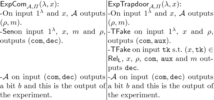
B Instantiation of a Secret Sharing Scheme

In this section we aim for a coding scheme $RS_N : \{0,1\}^{2n} \rightarrow (\{0,1\}^{k_2})^N$ that holds the $\lfloor N/3 \rfloor$-out-of-N secret sharing property. We show such construction for all parameters such that $\lfloor N/3 \rfloor \cdot k_2 \ge 2n$.

It turns out that the only we need for this purpose is the Reed-Solomon error correcting code c with following parameters:

• alphabet size $= 2^{k_2}$,

• block length $= N$,

• message length $M = 2 \cdot \lceil \frac{2n}{k_2} \rceil$.

Now our coding scheme may be defined as: $RS_N(m) = c(m || x)$, where x is a randomness of the same size as m.

We omit the simple proof that the above code actually holds the $\lfloor N/3 \rfloor$-out-of-N secret sharing property.

References

Aggarwal, D., Agrawal, S., Gupta, D., Maji, H.K., Pandey, O., Prabhakaran, M.: Optimal computational split-state non-malleable codes. In: Kushilevitz, E., Malkin, T. (eds.) TCC 2016, Part II. LNCS, vol. 9563, pp. 393–417. Springer, Heidelberg (2016). https://doi.org/10.1007/978-3-662-49099-0_15
Aggarwal, D., Dodis, Y., Lovett, S.: Non-malleable codes from additive combinatorics. In: STOC. ACM (2014)
Aggarwal, D., Döttling, N., Nielsen, J.B., Obremski, M., Purwanto, E.: Information theoretic continuously non-malleable codes in the constant split-state model. In: Presented at IMS Workshop on Information Theoretic Cryptography in NUS, Singapore (2016). Unpublished Manuscript, available on eprint
Aggarwal, D., Kazana, T., Obremski, M.: Inception makes non-malleable codes stronger. In: Kalai, Y., Reyzin, L. (eds.) TCC 2017. LNCS, vol. 10678, pp. 319–343. Springer, Cham (2017). https://doi.org/10.1007/978-3-319-70503-3_10
Agrawal, S., Gupta, D., Maji, H.K., Pandey, O., Prabhakaran, M.: Explicit non-malleable codes against bit-wise tampering and permutations. In: Gennaro, R., Robshaw, M. (eds.) CRYPTO 2015. LNCS, vol. 9215, pp. 538–557. Springer, Heidelberg (2015). https://doi.org/10.1007/978-3-662-47989-6_26
Agrawal, S., Gupta, D., Maji, H.K., Pandey, O., Prabhakaran, M.: A rate-optimizing compiler for non-malleable codes against bit-wise tampering and permutations. In: Dodis, Y., Nielsen, J.B. (eds.) TCC 2015. LNCS, vol. 9014, pp. 375–397. Springer, Heidelberg (2015). https://doi.org/10.1007/978-3-662-46494-6_16
Ball, M., Dachman-Soled, D., Kulkarni, M., Malkin, T.: Non-malleable codes for bounded depth, bounded fan-in circuits. Cryptology ePrint Archive, Report 2016/307 (2016). https://eprint.iacr.org/2016/307
Ball, M., Dachman-Soled, D., Kulkarni, M., Malkin, T.: Non-malleable codes from average-case hardness: Ac0, decision trees, and streaming space-bounded tampering. Cryptology ePrint Archive, Report 2017/1061 (2017). https://eprint.iacr.org/2017/1061
Barak, B.: Constant-round coin-tossing with a man in the middle or realizing the shared random string model. In: 43rd Symposium on Foundations of Computer Science (FOCS 2002), 16–19 November 2002, Vancouver, BC, Canada, Proceedings, pp. 345–355 (2002)
Broadnax, B., Döttling, N., Hartung, G., Müller-Quade, J., Nagel, M.: Concurrently composable security with shielded super-polynomial simulators. In: Coron, J.-S., Nielsen, J.B. (eds.) EUROCRYPT 2017. LNCS, vol. 10210, pp. 351–381. Springer, Cham (2017). https://doi.org/10.1007/978-3-319-56620-7_13
Broadnax, B., Fetzer, V., Müller-Quade, J., Rupp, A.: Non-malleability vs. CCA-security: the case of commitments. In: Abdalla, M., Dahab, R. (eds.) PKC 2018. LNCS, vol. 10770, pp. 312–337. Springer, Cham (2018). https://doi.org/10.1007/978-3-319-76581-5_11
Canetti, R., Lin, H., Pass, R.: Adaptive hardness and composable security in the plain model from standard assumptions. In: 51th Annual IEEE Symposium on Foundations of Computer Science, FOCS 2010, 23–26 October 2010, Las Vegas, Nevada, USA, pp. 541–550. IEEE Computer Society (2010)
Chandran, N., Goyal, V., Mukherjee, P., Pandey, O., Upadhyay, J.: Block-wise non-malleable codes. In: Chatzigiannakis, I., Mitzenmacher, M., Rabani, Y., Sangiorgi, D. (eds.) 43rd International Colloquium on Automata, Languages, and Programming, ICALP 2016, 11–15 July 2016, Rome, Italy, LIPIcs, vol. 55, pp. 31:1–31:14. Schloss Dagstuhl - Leibniz-Zentrum fuer Informatik (2016)
Chattopadhyay, E., Goyal, V., Li, X.: Non-malleable extractors and codes, with their many tampered extensions. In: Proceedings of the Forty-Eighth Annual ACM Symposium on Theory of Computing, pp. 285–298. ACM (2016)
Chattopadhyay, E., Zuckerman, D.: Non-malleable codes in the constant split-state model. iN: FOCS (2014)
Cheraghchi, M., Guruswami, V.: Capacity of non-malleable codes. In: Naor, M. (ed.) Innovations in Theoretical Computer Science, ITCS 2014, Princeton, NJ, USA, 12–14 January 2014, pp. 155–168. ACM (2014). https://doi.org/10.1145/2554797.2554814
Cheraghchi, M., Guruswami, V.: Non-malleable coding against bit-wise and split-state tampering. In: Lindell, Y. (ed.) TCC 2014. LNCS, vol. 8349, pp. 440–464. Springer, Heidelberg (2014). https://doi.org/10.1007/978-3-642-54242-8_19
Choi, S.G., Kiayias, A., Malkin, T.: BiTR: built-in tamper resilience. In: Lee, D.H., Wang, X. (eds.) ASIACRYPT 2011. LNCS, vol. 7073, pp. 740–758. Springer, Heidelberg (2011). https://doi.org/10.1007/978-3-642-25385-0_40
Ciampi, M., Ostrovsky, R., Siniscalchi, L., Visconti, I.: Concurrent non-malleable commitments (and More) in 3 rounds. In: Robshaw, M., Katz, J. (eds.) CRYPTO 2016. LNCS, vol. 9816, pp. 270–299. Springer, Heidelberg (2016). https://doi.org/10.1007/978-3-662-53015-3_10
Ciampi, M., Ostrovsky, R., Siniscalchi, L., Visconti, I.: Four-round concurrent non-malleable commitments from one-way functions. In: Katz, J., Shacham, H. (eds.) CRYPTO 2017. LNCS, vol. 10402, pp. 127–157. Springer, Cham (2017). https://doi.org/10.1007/978-3-319-63715-0_5
Ciampi, M., Persiano, G., Scafuro, A., Siniscalchi, L., Visconti, I.: Improved OR-composition of sigma-protocols. In: Kushilevitz, E., Malkin, T. (eds.) TCC 2016. LNCS, vol. 9563, pp. 112–141. Springer, Heidelberg (2016). https://doi.org/10.1007/978-3-662-49099-0_5
Coretti, S., Maurer, U., Tackmann, B., Venturi, D.: From single-bit to multi-bit public-key encryption via non-malleable codes. In: Dodis, Y., Nielsen, J.B. (eds.) TCC 2015. LNCS, vol. 9014, pp. 532–560. Springer, Heidelberg (2015). https://doi.org/10.1007/978-3-662-46494-6_22
Damgård, I., Kazana, T., Obremski, M., Raj, V., Siniscalchi, L.: Continuous NMC secure against permutations and overwrites, with applications to CCA secure commitments. Cryptology ePrint Archive, Report 2018/596 (2018). https://eprint.iacr.org/2018/596
Dolev, D., Dwork, C., Naor, M.: Non-malleable cryptography (extended abstract). In: Proceedings of the 23rd Annual ACM Symposium on Theory of Computing, 5–8 May 1991, New Orleans, Louisiana, USA, pp. 542–552 (1991)
Döttling, N., Nielsen, J.B., Obremski, M.: Information theoretic continuously non-malleable codes in the constant split-state model. iN: Presented at IMS Workshop on Information Theoretic Cryptography in NUS, Singapore (2016). Unpublished Manuscript, available on eprint
Dziembowski, S., Kazana, T., Obremski, M.: Non-malleable codes from two-source extractors. In: Canetti, R., Garay, J.A. (eds.) CRYPTO 2013. LNCS, vol. 8043, pp. 239–257. Springer, Heidelberg (2013). https://doi.org/10.1007/978-3-642-40084-1_14
Dziembowski, S., Pietrzak, K., Wichs, D.: Non-malleable codes. In: ICS, pp. 434–452. Tsinghua University Press (2010)
Faust, S., Mukherjee, P., Nielsen, J.B., Venturi, D.: Continuous non-malleable codes. In: Lindell, Y. (ed.) TCC 2014. LNCS, vol. 8349, pp. 465–488. Springer, Heidelberg (2014). https://doi.org/10.1007/978-3-642-54242-8_20
Faust, S., Mukherjee, P., Nielsen, J.B., Venturi, D.: A tamper and leakage resilient von neumann architecture. In: Katz, J. (ed.) PKC 2015. LNCS, vol. 9020, pp. 579–603. Springer, Heidelberg (2015). https://doi.org/10.1007/978-3-662-46447-2_26
Faust, S., Mukherjee, P., Venturi, D., Wichs, D.: Efficient non-malleable codes and key-derivation for poly-size tampering circuits. In: Nguyen, P.Q., Oswald, E. (eds.) EUROCRYPT 2014. LNCS, vol. 8441, pp. 111–128. Springer, Heidelberg (2014). https://doi.org/10.1007/978-3-642-55220-5_7
Gennaro, R., Lysyanskaya, A., Malkin, T., Micali, S., Rabin, T.: Algorithmic tamper-proof (ATP) security: theoretical foundations for security against hardware tampering. In: Naor, M. (ed.) TCC 2004. LNCS, vol. 2951, pp. 258–277. Springer, Heidelberg (2004). https://doi.org/10.1007/978-3-540-24638-1_15
Goyal, V.: Constant round non-malleable protocols using one way functions. In: Proceedings of the 43rd ACM Symposium on Theory of Computing, STOC 2011, San Jose, CA, USA, 6–8 June 2011, pp. 695–704 (2011)
Goyal, V., Lee, C., Ostrovsky, R., Visconti, I.: Constructing non-malleable commitments: A black-box approach. In: 53rd Annual IEEE Symposium on Foundations of Computer Science, FOCS 2012, New Brunswick, NJ, USA, 20–23 October 2012, pp. 51–60 (2012)
Goyal, V., Lin, H., Pandey, O., Pass, R., Sahai, A.: Round-efficient concurrently composable secure computation via a robust extraction lemma. In: Dodis, Y., Nielsen, J.B. (eds.) TCC 2015. LNCS, vol. 9014, pp. 260–289. Springer, Heidelberg (2015). https://doi.org/10.1007/978-3-662-46494-6_12
Goyal, V., Pandey, O., Richelson, S.: Textbook non-malleable commitments. In: Wichs, D., Mansour, Y. (eds.) Proceedings of the 48th Annual ACM SIGACT Symposium on Theory of Computing, STOC 2016, Cambridge, MA, USA, 18–21 June 2016, pp. 1128–1141. ACM (2016)
Goyal, V., Richelson, S., Rosen, A., Vald, M.: An algebraic approach to non-malleability. In: 55th IEEE Annual Symposium on Foundations of Computer Science, FOCS 2014, Philadelphia, PA, USA, 18–21 October 2014, pp. 41–50 (2014)
Jafargholi, Z., Wichs, D.: Tamper detection and continuous non-malleable codes. In: Dodis, Y., Nielsen, J.B. (eds.) TCC 2015. LNCS, vol. 9014, pp. 451–480. Springer, Heidelberg (2015). https://doi.org/10.1007/978-3-662-46494-6_19
Khurana, D.: Round optimal concurrent non-malleability from polynomial hardness. In: Kalai, Y., Reyzin, L. (eds.) TCC 2017. LNCS, vol. 10678, pp. 139–171. Springer, Cham (2017). https://doi.org/10.1007/978-3-319-70503-3_5
Khurana, D., Sahai, A.: How to achieve non-malleability in one or two rounds. In: Umans, C. (ed.) 58th IEEE Annual Symposium on Foundations of Computer Science, FOCS 2017, Berkeley, CA, USA, 15–17 October 2017, pp. 564–575. IEEE Computer Society (2017)
Kiyoshima, S.: Round-efficient black-box construction of composable multi-party computation. In: Garay, J.A., Gennaro, R. (eds.) CRYPTO 2014. LNCS, vol. 8617, pp. 351–368. Springer, Heidelberg (2014). https://doi.org/10.1007/978-3-662-44381-1_20
Kiyoshima, S.: Statistical concurrent non-malleable zero-knowledge from one-way functions. In: Gennaro, R., Robshaw, M. (eds.) CRYPTO 2015. LNCS, vol. 9216, pp. 85–106. Springer, Heidelberg (2015). https://doi.org/10.1007/978-3-662-48000-7_5
Li, X.: Improved non-malleable extractors, non-malleable codes and independent source extractors. In: STOC (2017). https://arxiv.org
Lin, H., Pass, R.: Constant-round non-malleable commitments from any one-way function. In: Fortnow, L., Vadhan, S.P. (eds.) Proceedings of the 43rd ACM Symposium on Theory of Computing, STOC 2011, San Jose, CA, USA, 6–8 June 2011, pp. 705–714. ACM (2011)
Lin, H., Pass, R.: Black-box constructions of composable protocols without set-up. In: Safavi-Naini, R., Canetti, R. (eds.) CRYPTO 2012. LNCS, vol. 7417, pp. 461–478. Springer, Heidelberg (2012). https://doi.org/10.1007/978-3-642-32009-5_27
Lin, H., Pass, R., Soni, P.: Two-round and non-interactive concurrent non-malleable commitments from time-lock puzzles. In: Umans, C. (ed.) 58th IEEE Annual Symposium on Foundations of Computer Science, FOCS 2017, Berkeley, CA, USA, 15–17 October 2017, pp. 576–587. IEEE Computer Society (2017)
Liu, F.-H., Lysyanskaya, A.: Tamper and leakage resilience in the split-state model. In: Safavi-Naini, R., Canetti, R. (eds.) CRYPTO 2012. LNCS, vol. 7417, pp. 517–532. Springer, Heidelberg (2012). https://doi.org/10.1007/978-3-642-32009-5_30
Pass, R., Rosen, A.: New and improved constructions of non-malleable cryptographic protocols. In: Gabow, H.N., Fagin, R. (eds.) Proceedings of the 37th Annual ACM Symposium on Theory of Computing, Baltimore, MD, USA, 22–24 May 2005, pp. 533–542. ACM (2005)
Pass, R., Wee, H.: Constant-round non-malleable commitments from sub-exponential one-way functions. In: Gilbert, H. (ed.) EUROCRYPT 2010. LNCS, vol. 6110, pp. 638–655. Springer, Heidelberg (2010). https://doi.org/10.1007/978-3-642-13190-5_32
Wee, H.: Black-box, round-efficient secure computation via non-malleability amplification. In: 51th Annual IEEE Symposium on Foundations of Computer Science, FOCS 2010, 23–26 October 2010, Las Vegas, Nevada, USA, pp. 531–540. IEEE Computer Society (2010)
Chung, K-M., Pass, R., Seth, K.: Non-black-box simulation from one-way functions and applications to resettable security. In: Boneh, D., Roughgarden, T., Feigenbaum, J. (eds.) Symposium on Theory of Computing Conference, STOC 2013, Palo Alto, CA, USA, 1–4 June 2013, pp. 231–240. ACM (2013). https://doi.org/10.1145/2488608.2488638
Acknowledgments
We thank Michele Ciampi for several discussions on the applications of our CNMC.
Author information
Authors and Affiliations
Corresponding author
Editor information
Editors and Affiliations