Exploring Errors in Reading a Visualization via Eye Tracking Models Using Stochastic Geometry

Abstract

Information visualizations of quantitative data are rapidly becoming more complex as the dimension and volume of data increases. Critical to modern applications, an information visualization is used to communicate numeric data using objects such as lines, rectangles, bars, circles, and so forth. Via visual inspection, the viewer assigns numbers to these objects using their geometric properties of size and shape. Any difference between this estimation and the desired numeric value we call the “visual measurement error”. The research objective of this paper is to propose models of the visual measure error utilizing stochastic geometry. The fundamental technique in building our models is the conceptualization of eye fixation points as might be determined by an eye-tracking experiment of viewers estimating size and shape of a visualization’s object configurations. The fixation points are first considered as a stochastic point process whose characteristics require comment before proceeding to the statistical shape analysis of the visualization. Once clarified the fixation points are reinterpreted as a sampling of the shape and size of the landmark configurations of geometric landmarks on the visualization. The ultimate end of these models is to find optimal shape and size parameters leading to minimum visual measurement error.

1 Introduction

Information visualizations of quantitative data are rapidly becoming more complex as the dimension and volume of data increases [1]. Critical to modern applications, an information visualization is used to communicate numeric data using objects such as lines, rectangles, bars, circles, and so forth. Via visual inspection, the viewer assigns numbers to these objects using their geometric properties of size and shape [2]. Any difference between this estimation and the desired numeric value we call the “visual measurement error”. The research objective of this paper is to propose models of the visual measurement error utilizing stochastic geometry. The fundamental technique in building these models is to abstract the accumulation of eye fixation points produced during an eye-tracking experiment [3]. Participants will be asked to “measure” the size of objects with the visualization configuration. The fixation points are first viewed as a spatial point pattern of a spatial stochastic point process. We will look at its properties and see various shortcomings when applied to the analysis of the structure of information visualization. At this point, the research takes a novel turn. The fixation points are reinterpreted as a sampling of the landmark configuration of a visualization construct. The study of visualization measurement error will utilize Bookstein’s analysis of the size and shape of a triangle. An error model will be given under strongly simplifying assumptions.

2 Eye Tracking Analysis of Information Visualization

We pose the following abstract usability experiment. A group of people is shown the simple bar chart seen in Fig. 1. They are given the task of measuring bar A against the ruler and estimate it’s “height” according to the ruler’s scale. (We will use the term height as if the scale where in inches.). While doing so they are monitored using an eye tracker. Previous related research [22] showed the fixation points of the search appeared as in the right-hand side of Fig. 1. Of course, the striking feature is the formation of three clustered regions. To understand the information stored in these clusters, it is necessary to build a mathematical framework to describe the experiment. We will follow the lines of development and definitions used in [4] and [5].

Fig. 1.

The left picture shows the visualization. The right picture shows the fixation points from the eye tracking data.

Denote $\tilde{S}$ as a set of fixation points in ${\mathbb{R}}^{2}$. Mathematically, it is viewed as a spatial point pattern.

Definition 1:

A spatial point pattern is a set of points in the plane denoted as:

$$ \{ {\mathbf{x}}_{1} ,{\mathbf{x}}_{2} , \ldots ,{\mathbf{x}}_{k} \} $$

(1)

where

$$ \varvec{x}_{j} = \left[ {\begin{array}{*{20}c} {x_{j} } \\ {y_{j} } \\ \end{array} } \right]. $$

Each person in the experiment will compare the Bar A to the axis to the left as shown in Fig. 1 then report the bar’s height they observed, $\hat{h}.$ Meanwhile, we collected the data produced by the eye tracker. In an idealized sense, we have captured the formation of a spatial point pattern $\hat{S}$ during the measurement process. For each test subject, we obtain the pairing $(\hat{S},\hat{h})$. If there are $n$ participants in the experiment, we collect a set of information of the form

$$ \{ (\tilde{S}_{1} ,\tilde{h}_{1} ),(\tilde{S}_{2} ,\tilde{h}_{2} ), \ldots ,(\tilde{S}_{n} ,\tilde{h}_{n} )\} . $$

(2)

2.1 Addressing Error

Error is the difference between $h$ and $\tilde{h}$. The determination of the measurement $\tilde{h}$ is the result of a complex system of interactions between the eye, brain, and visualization. Identifying every possible physiological and cognitive effect leading to $\tilde{h}$ is beyond our current level of understanding [2]. However, it is the hope of usability research that many of these complexities are encapsulated in the eye’s motion during the measurement process [6, 7]. Eye tracking can be view then as an indirect sampling of unobservable processes. Unless the measurement of $\tilde{h}$ is the result of a completely random process, it seems reasonable any underlying process could be influenced by observable factors such as lengths, widths, and areas. Expressing this influence will occupy the rest of this paper.

3 Modeling

The purpose of this research is to propose models of visual measurement error. Some models we will simply offer for future consideration. For other models, we will discuss their reasonableness. Since we are using eye-tracking experiments as our inspirational gateway into this topic, all of our models begin with a spatial point pattern. Based on this, our models can be divided into approaches: spatial point processes and spatial shape processes. Introductory ideas, including motivation, and some basic results will be included in this section. The details of more involved models will be deferred to the particular application. (We assume the reader is familiar with basic probabilities theory a little measure theory.)

4 Stochastic Point Processes

4.1 Basic Premises

For beginners, the mathematical definition of a point process is surprising complex (see [8] or [9]). To simplify our situation as much as possible, we will consider a point process a random mechanism whose outcomes are spatial point patterns. Believing there are only a finite number of fixation points on a visualization, we restrict attention to finite point processes; bringing us to the following definition [4]:

Definition 2:

A finite point process ${\mathbf{X}}$ is a random mechanism for which,

• 1. Every possible outcome is a spatial point pattern with a finite number of points,

• 2. For all test sets (closed and bounded) subsets $B$ of ${\mathbb{R}}^{2}$, the number of points of ${\mathbf{X}}$ in $B$ is finite, denoted as $N({\mathbf{X}} \cap B)$, is a well-defined random variable.

In considering spatial point pattern realizations of the underlying point process, people seek answers to standards questions. Is the density (number of points per area) constant? Are the points distributed “evenly” or “uniformly” across some region? Are there voids (empty regions)? Has the data clustered? Is there evidence of point or area interaction? What is the distribution function of the random processes at play? We continue by following the presentation of Baddeley, Rubak, and Turner in their excellent book [4].

4.2 Complete Spatial Randomness

Our first objective is to define complete spatial randomness (CSR). This is important because our approach to building models is inspired by eye tracking. It is reasonable to believe seemingly random motion of the eye demonstrates a certain lack of understanding or interest on the part of the viewer and will provide little insight into geometric structure.

Formulating CSR requires several characteristics of the finite point distribution. We want the spatial pattern to have no preferred location so they the points appear to be distributed uniformly. This introduces the concept of a spatial probability density. To comply with Definition 2 part (2), we will need the probability distribution of the count functions $N(X \cap B).$

We begin with the notion of a spatial pattern being uniformly distributed. To keep things simple, we begin considering how to place a point in a window set $W$ uniformly. First, suppose that location of the single point $(u_{1} ,u_{2} )$ in Fig. 2 is expressed by random variables $U_{1}$ and $U_{2}$ with joint probability distribution $\lambda (u_{1} ,u_{2} )$. The probability that $U = (U_{1} ,U_{2} )$ lies in the so-called test set $B$ is

Fig. 2.

Uniformly distributed random points. Right: point is in a test set. left: point is given coordinates as realization of random variables

$$ {\mathbb{P}}(U \in B) = \int\limits_{B} {\lambda (u_{1} ,u_{2} )d} u_{1} du_{2} . $$

(3)

Since the Lebesgue measure is non-atomic, Eq. (3) is different than

$$ {\mathbb{P}}((U_{1} ,U_{2} ) = (u_{1} ,u_{2} )) = 0 $$

(4)

If we require the probability density function $\lambda (u_{1} ,u_{2} )$ to be a bivariate uniform distribution on $W$, we have

$$ \lambda (u_{1} ,u_{2} ) = \left\{ {\begin{array}{*{20}c} {1/\left| W \right|} & {(u_{1} ,u_{2} ) \in W} \\ 0 & {\text{otherwise}} \\ \end{array} } \right. $$

(5)

Here and elsewhere $\left| W \right|$ is the two-dimensional Lebesgue measure of $W$, which is its area. Using Eq. (5) in Eq. (3),

$$ {\mathbb{P}}(U \in B) = \int\limits_{B} {\lambda (u_{1} ,u_{2} )d} u_{1} du_{2} = \frac{1}{W}\int\limits_{B} 1 du_{1} du_{2} = \frac{\left| B \right|}{\left| W \right|}. $$

(6)

This is intuitively pleasing as the probability a spatial point “hits” the test set is the proportion of area it occupies. Let us call this probability $p(B)$.

Suppose now that we wish to place $n$ points uniformly in $W$. To this end, we define a finite point process ${\mathbf{X}} = \{ U_{1} ,U_{2} , \ldots ,U_{n} \}$ where each $U_{j}$ is a uniformly distribution random point as per the proceeding the paragraph. Let $B$ be a test set. If we associate a “hit” with a “success”, we are counting the number of successes out of $n$ trials. If we suppose that each trial is independent of the others but share the same probability of hitting $B$, we have from Eq. (6)

$$ {\mathbb{P}}(U_{j} \in B) = \left| B \right|/\left| W \right| = p(B){\text{ for }}i = 1,2, \ldots ,n. $$

(7)

From this, we quickly recognize that $N({\mathbf{X}} \cap B)$ has the binomial distribution [10]

$$ {\mathbb{P}}(N({\mathbf{X}} \cap B) = k) = \frac{n!}{{k!\left( {n - k} \right)!}}p(B)^{k} (1 - p(B))^{n - k} . $$

(8)

The expected value of a binomial process [10] is

$$ {\mathbb{E}}[N({\mathbf{X}} \cap B)] = np(B). $$

(9)

From Eq. (6),

$$ {\mathbb{E}}[N({\mathbf{X}} \cap B)] = n({\mathbf{X}})\frac{\left| B \right|}{\left| W \right|} = \frac{{n({\mathbf{X}})}}{\left| W \right|}\left| B \right| = \hat{\lambda }({\mathbf{X}})\left| B \right|. $$

(10)

Here

$$ \hat{\lambda }({\mathbf{X}}) = \frac{{n({\mathbf{X}})}}{\left| W \right|}. $$

(11)

The notation $n({\mathbf{X}})$ means the number of points in the process ${\mathbf{X}}$. Likewise, $\hat{\lambda }({\mathbf{X}})$ is the expected number of points in a set $B$. We call this the intensity of ${\mathbf{X}}.$

The utility of intensity warrants a formal definition. For a general point process ${\mathbf{X}},$

$$ {\mathbb{E}}[N({\mathbf{X}} \cap B)] = \int\limits_{B} {\lambda (u)du} $$

(12)

If it exists, $\lambda (u)$ is called the intensity function. We call a process homogeneous if the intensity is constant,

$$ {\mathbb{E}}[N({\mathbf{X}} \cap B)] = \lambda \left| B \right|. $$

(13)

A final issue of primary importance concerns the probability distribution of the random variable $N({\mathbf{X}} \cap B)$ as referred to in (2) of Definition 2. Assuming the process is homogeneous; using Eq. (13) it can be shown $N({\mathbf{X}} \cap B)$ Poisson distributed [11].

Definition 3:

A non-negative integer-valued random variable $Y$ has the Poisson distribution [ 10 ] (denoted $P(\mu )$ ) if

$$ {\mathbb{P}}[Y = k] = \text{e}^{ - \mu } \frac{{\mu^{k} }}{k!}{\text{ for }}k = 0,1,2, \ldots $$

(14)

An important property of this distribution is

$$ {\mathbb{E}}[{\mathbf{Y}}] = \mu {\text{ and V}}[{\mathbf{Y}}] = \mu $$

(15)

We are now ready to define what it means for process to be spatially random [4].

Definition 4:

A homogenous Poisson Point Process ${\mathbf{X}}$ with $\lambda > 0$ has the following properties:

• 1. Poisson Counts: the random variable $N({\mathbf{X}} \cap B)$ has a Poisson distribution $P(\mu )$ with

  $$ \mu (B) = \int\limits_{B} {\lambda (u)du} = \lambda \left| B \right| ; $$

  (16)

• 2. Homogeneous Intensity: the expected number of points hitting a test set $B$ is

  $$ {\mathbb{E}}[N({\mathbf{X}} \cap B)] = \lambda \left| B \right|; $$

  (17)

• 3. Independence: if $B_{1} ,B_{2} , \ldots$ are disjoint regions of the plane, then $N({\mathbf{X}} \cap B_{1} ),N({\mathbf{X}} \cap B_{2} ), \ldots$ are independent random variables.

  Fig. 3.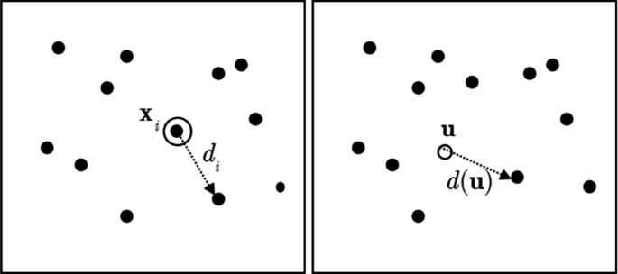

  

  Right: Shows the nearest neighbor distance is a from point to point in the process. Left: shows the empty-space distance is from a fixed location to a point in the process

5 Point Process Error Models

Returning to the eye tracking experiment, we are asking test subjects to visually measure the height of a bar $(h)$ using a ruler which is $d$ units away. As is suggested in the picture on the right in Fig. 1, the measurement effort leads to the formation of an eye tracking spatial point pattern as a cluster around the point ${\mathbf{h}}$. (We will use the notation ${\mathbf{h}} = (0,h)$ when referring to the point in the plane and $h$ for its length.). From out of this cluster, the subject produces a number $\hat{h}_{j}$ most often different from $h$ leading to a difference $\varepsilon_{j}$, which we are calling the visual measurement error.

To quantify this, we begin with a spatial point pattern given in Definition 1. In order to specify the magnitude $\varepsilon_{j}$, we need an appropriate distance measure [4]. A natural approach is the classic Euclidean norm for the plane and use it to define the pairwise distances

$$ d_{ij} = \left\| {{\mathbf{x}}_{i} - {\mathbf{x}}_{j} } \right\| = \sqrt {(x_{i} - x_{j} )^{2} + (y_{i} - y_{j} )^{2} } $$

(18)

This distance is defined independent of the eye tracking behavior, which is a concern, since we are trying to understand the impact of visualization design on the visual measurement error.

We are modelling through the lens of the eye tracking patterns. Therefore, it is reasonable we consider whether there is a characteristic of the pattern that reveals the estimated height. This means we seek a “process specific” distance measure. Choosing a point in the process, say ${\mathbf{x}}_{i}$, we define the nearest neighbor distance (Fig. 3) as

$$ d_{i} = {\rm min}_{j \ne i} d_{ij} $$

(19)

In our situation, we need to identify areas of interest (AOI) and measure how the process behaves in and around them. For example, we might question if the process enters a disk around ${\mathbf{h}}$. This leads us to a final measure of distance. The empty-space distance

$$ d({\mathbf{u}}) = {\rm min}_{j} \left\| {{\mathbf{u}} - {\mathbf{x}}_{j} } \right\| . $$

(20)

It is the distance from a fixed reference location ${\mathbf{u}}$ to the nearest point in the process.

6 Analysis of Fixation Point Process

The first question we must face is whether the fixation points are randomly generated by the eye. In what follows, we do two things. First, we consider whether a reasonable error model derived, assuming the fixation points, satisfies complete spatial randomness (CSR) criteria. Second, we will show that CSR does not provide any of the desired implications of geometric structure.

6.1 Nearest Neighbor

Let us consider the cluster of fixation points about the point ${\mathbf{h}} = (0,h)$. The experiment asks the test subject is to estimate $h$. Suppose that $\hat{h}$ is returned. Odds are they are different. We have been calling this the visual measurement error. We have now reached the beginning of the modelling process. The first issue we face is to define the error metric to be used. This is more challenging than it seems. Of course, the distance $\left| {h - \hat{h}} \right|$ is obvious but it contains no information about the point process.

As a starting point, we will suppose fixation points form a homogenous Poisson process called ${\mathbf{X}}$. To include the point of ${\mathbf{X}}$ in the measurement process, we could reason as follows. While we do not know how the brain does the visual measurement, it seems safe to believe the points of ${\mathbf{X}}$ nearest ${\mathbf{h}}$ contribute the most information. Suppose we place a disk around ${\mathbf{h}}$ with radius $\varepsilon$. We then increase the radius until the disk makes contact with a point of ${\mathbf{X}}$. This is the empty space distance discuss above. It is a random variable with a known probability distribution function [9]

$$ H_{S} (r) = 1 - \exp ( - \lambda \pi r^{2} ) . $$

(21)

Using this, we derive the mean empty space distance is

$$ m_{s} = \frac{1}{2\sqrt \lambda }. $$

(22)

This tells us that the expected difference between the observed and actual height of the bar. Is this a good error model? We note the mean is independent of $h$. Another feature is the mean is proportional to the inverse square root of the intensity $\lambda$. This is curious. If we increase by four the number of points about ${\mathbf{h}}$, we will reduce the error by only a half. It would seem that increasing the amount of visual activity by so much produced too little.

6.2 Stationary Process

It already seems as though modeling eye tracking as a spatially random point process has issues. We now see another. CSR is stationary or translation invariant [4]. Formally, we say a point process ${\mathbf{X}}$ stationary if for every vector ${\mathbf{v}}$, the process ${\mathbf{X}} + {\mathbf{v}}$ has the same statistical properties as ${\mathbf{X}}$.

Suppose that ${\mathbf{X}}$ is a stationary process associated with an eye tracking experiment. Consider the vector ${\mathbf{v}} = (d,0)$ and form the translated process ${\mathbf{X^{\prime}}} = {\mathbf{X}} + {\mathbf{v}}$. Being stationary ${\mathbf{X^{\prime}}}$ has the same properties at $(d,h)$ as ${\mathbf{X}}$ at $(0,h)$. This would say that the error inherent in measuring the bar height by looking at the ruler is no different than looking at the bar.

Does this seem reasonable? Let us perform a simple analysis. If we think of the eyes as tracing gaze paths generally along $y = h$ from the bar to the ruler, it is seems plausible the paths can be bounded by a triangle¹, as show in Fig. 4. This shows that a small angle error in “shooting” a path from the bar to ruler can result in an error of the form

Fig. 4.

This suggests that if the eye makes a small error in tracing along the line from the bar to the ruler, then the resulting error grows linearly in the distance.

$$ \varepsilon = d\tan (\theta ). $$

(23)

While not rigorous, it supports a belief the visual measurement error depends on the distance of the bar from the ruler.

6.3 Inhomogeneous Processes

Based on the preceding discussion, homogeneous point processes make poor models of visual measurement error. Therefore, our next step along this path is to find a good model with a non-constant intensity. The numerical covariate of the distance from a selected point to say $(0,h)$ might serve as an excellent effect to build into the model. It could represent the challenge/ease one has in concentrating on ${\mathbf{h}}$. This is a good subject to explore in upcoming work.

The most obvious characteristic we have not addressed in our error modeling discussion is that the fixation points cluster around areas critical to measuring the height of bar A. See Fig. 1. Cluster formation is typically modelled in steps similar to growing a forest. First, a process places parent points (trees). Then in a region about the parent, child points (seedlings) are placed according to another distribution. Most of the popular cluster models assign independence to these clusters meaning what happens around one tree does not affect another. (Trees are not interacting with each other.). This confronts another issue. Are the clusters are spatially correlated? Correlation is likely as judging the height of the bar requires looking at both the bar and the ruler.

Gathering our thoughts, a useful cluster model needs the parents to be fixed with clusters forming around them. Consideration needs to be given to how the children in different clusters interact. For example, the eye fixating on a point near the bar might then quickly skip to the ruler. One approach to modeling this skipping behavior is to choose a child in each cluster and connect them by line. The simplest way to connect all three clusters is to build triangles with vertices in each point cluster.

This, then, has led us to statistical shape processes as a reasonable basis for visual measurement error modeling.

7 Stochastic Geometry Processes

We are exploring the relationship between visual measurement error and the geometrical shape of subcomponents of a visualization. In the first part, we viewed the eye as sampling data at points in the picture. We then built models utilizing random point processes. These mechanisms place points “randomly” around the plane based on underlying premises.

We now make a major change of philosophy. While we track fixation points, we suggest that the brain is seeing geometry in our case triangles. As show conceptually in Fig. 5, we propose to consider a mechanism placing triangles randomly on the visualization. To the best of our knowledge, stochastic geometry has yet to be utilized in usability analysis of information visualizations.

Fig. 5.

A random triangle process

To this end, we must introduce the notions of landmark configurations and shape. We follow the approach introduced by Kendall [13]. Herein, we use the presentation by Dryden and Mardia [14].

7.1 Landmark Configurations

Consider a family of bar graphs. Any single bar graph is a collection of rectangles positioned on some (normally unspecified) coordinate system. In order to relate the family of bar graphs to each other, we introduce landmarks [14, 15].

As shown in Fig. 6 the landmarks are chosen as the corners of the bar. The landmarks ensure that a family of bar graphs, which varies the parameters $d$, $w$ and $h$, maps the corners correctly. In practice, a heuristic approach is taken to landmark selection [14]. For visualizations of count data, landmarks might be assigned to corners of rectangles, the intersection of lines and so forth.

Fig. 6.

The landmark configuration of a single bar with the triangle shape needed to capture error in visual measurement

Definition 5:

A landmark is a point of correspondence on each object that matches between and within populations.

Definition 6:

A configuration is the set of landmarks on a particular object:

$$ \{ {\mathbf{x}}_{1} ,{\mathbf{x}}_{2} , \ldots ,{\mathbf{x}}_{k} \} $$

(24)

For the planar case,

$$ \varvec{x}_{j} = \left( {\begin{array}{*{20}c} {x_{j} } \\ {y_{j} } \\ \end{array} } \right) $$

(25)

7.2 Shape and Size

Consider the triangle in Fig. 6. It seems reasonable that where the triangle occurs in the visualization does not affect its intrinsic geometric properties. In most bar graphs, the bar rectangles are either horizontal or vertical. Which one is used will cause the triangle to rotate. Again, one would suspect that rotation does not change the intrinsic properties of the triangle. As a viewer can zoom in or out, the geometric properties should remain unchanged. Translation, rotation, and scaling comprise the so-called Euclidean similarity transformations (see [14] for precise definitions).

With these ideas in mind, Kendall [13] proposed the following definitions of shape and size.

Definition 7:

Shape is all of the geometric information that remains after location, scale, and rotational effects are filtered out of an object.

Definitions require examples. Let us consider the triangle in Fig. 7. If it is translated, the angles do not change. If it is rotated, the angles do not change. If the triangle is dilated, the angles do not change. Hence, the angles invariant under the set of Euclidean similarity transformations. Another item to note is that $\alpha + \beta + \gamma = 180^{ \circ }$. Therefore, we need to know only two of the three angles to identify the shape of the triangle. This little observation was made profound by Kendall ([16,17,18]). In practice however, using all three angles as shape parameters has proven to be problematic particularly in the possibility of a degenerate case of a flat triangle. We will use the shape parameters proposed by Bookstein [15, 19].

Fig. 7.

The internal angles of a triangle describe the shape of the triangle.

Definition 8:

The size-and-shape is all of the geometric information that remains after location and rotational effects are filtered out of an object.

The notion of the size of an object being is invariant over scaling is odd. It means that size is internal. A common version is the sum of the lengths from a vertex to the centroid. We will introduce another in the next section.

7.3 Bookstein’s Approach to Triangles

Rather than continuing this discussion in an abstract sense, let us focus on the case of the triangles in the plane. We will use Bookstein’s approach [15, 19] as it illustrate the concept of stochastic triangles fairly well.

We begin the following statistical model:

$$ {\mathbf{p}}_{k} = {\mathbf{z}}_{k} + {\mathbf{d}}_{k} {\text{ for }}k = 1,2,3 $$

(26)

We interpret ${\mathbf{p}}_{k}$ as the sampling of kth landmark ${\mathbf{z}}_{k}$, in which encountered an error of ${\mathbf{d}}_{k}$. In coordinate form

$$ \left[ {\begin{array}{*{20}c} {x_{k} } \\ {y_{k} } \\ \end{array} } \right] = \left[ {\begin{array}{*{20}c} {z_{kx} } \\ {z_{ky} } \\ \end{array} } \right] + \left[ {\begin{array}{*{20}c} {d_{kx} } \\ {d_{ky} } \\ \end{array} } \right]{\text{ for }}k = 1,2,3 $$

(27)

The error terms are random variables with a normal distribution,

$$ d_{kx} ,d_{ky} \sim N(0,\sigma_{k}^{2} ) $$

(28)

As shown in Fig. 8 left picture, there are three clusters of fixation points. For simplicity, we will assume that each has $M$ of these. We draw a point from each cluster to form the j^th sample configuration

Fig. 8.

Left: Connect any three points from each cluster. Right: Bookstein’s approach to a random configuration

$$ {\mathbf{P}}^{j} = \{ {\mathbf{p}}_{1}^{j} ,{\mathbf{p}}_{2}^{j} ,{\mathbf{p}}_{3}^{j} \} {\text{ for }}j = 1, \ldots ,n{\text{ where }}n = M^{3} . $$

(29)

What can we hope to learn from this information? We will not be able to recover the original landmarks since our data might have been subject to translation, rotation, or scaling changes. Therefore, we must focus on the size and shape parameters. For the purpose of this paper, size characteristics will suffice.

7.4 Configuration Sizes

In our original triangle derived from the eye tracking experiment, we have

$$ z_{1} = (d + w,0) \, z_{2} = (d + w,h) \, z_{{}} = (d + w,h) $$

(30)

As nothing in what is to follow will distinguish $d$ from $w$, let us relabel $d + w$ as $d$.

By Eq. (17),

$$ d_{12} = \left\| {{\mathbf{z}}_{2} - {\mathbf{z}}_{1} } \right\| = h\ \ d_{23} = \left\| {{\mathbf{z}}_{3} - {\mathbf{z}}_{2} } \right\| = d\ \ d_{13} = \left\| {{\mathbf{z}}_{3} - {\mathbf{z}}_{1} } \right\| = \sqrt {d^{2} + h^{2} } $$

(31)

Using the data from the j^th configuration, we estimate the distances with

$$ \hat{d}^{j}_{12} = \left\| {{\mathbf{p}}_{2}^{j} - {\mathbf{p}}_{1}^{j} } \right\|\ \ \hat{d}^{j}_{23} = \left\| {{\mathbf{p}}_{3}^{j} - {\mathbf{p}}_{2}^{j} } \right\|\ \ \hat{d}^{j}_{13} = \left\| {{\mathbf{p}}_{3}^{j} - {\mathbf{p}}_{1}^{j} } \right\| $$

(32)

Let us now integrate the stochastic elements. In Fig. 9, we show a simplified calculation of the type in Eq. (32) in which we translated to the origin. By Eq. (28),

Fig. 9.

Approximating the edge length with the distance between sample points

$$ \begin{aligned} \eta = d_{2x} - d_{1x} \, \eta \sim {\text{N(0,}}\sigma_{12}^{2} ) \, \hfill \\ \xi = d_{2y} - d_{1y} \, \xi \sim {\text{N(0,}}\sigma_{12}^{2} ) \, \hfill \\ \end{aligned} $$

(33)

With $\sigma_{12}^{2} = \sigma_{1}^{2} + \sigma_{2}^{2}$

In Fig. 9, we show how an edge of the triangle is calculated based upon the eye tracking fixation points. The edge shown corresponds to the height of the Bar A. The random variable length $D$ represents the measure reported by the test subject so our visual measurement error corresponds to $\left| {h - D} \right|$.

The quantity $D/\sigma_{12}$, introduced in Fig. 9, has the non-central Chi-distribution with 2 degrees of freedom and non-centrality parameter $\lambda = h^{2} /\sigma_{12}^{2}$ [5]. Its probability density function [20] is

$$ \frac{x}{{\sigma^{2} }}\exp \left( {\frac{{ - (x^{2} + h^{2} )}}{{2\sigma^{2} }}} \right)\text{I}_{0} \left( {\frac{xh}{{\sigma^{2} }}} \right). $$

(34)

Here $\text{I}_{0}$ is the Modified Bessel Function of the First Kind [21] with series expansion

$$ 1 + \frac{{x^{2} }}{4} + \frac{{x^{4} }}{64} + \frac{{x^{6} }}{2304} + \frac{{x^{8} }}{147456} + \frac{{x^{10} }}{14745600} + O\left( {x^{11} } \right) $$

(35)

The mean of the distribution of $D$ [20] as shown in Fig. 9 is

$$ {\mathbb{E}}[D] = \sqrt {\frac{\pi }{2}} *\sigma *\text{L}_{1/2} \left( { - \frac{{h^{2} }}{{2\sigma^{2} }}} \right) $$

(36)

In our notation, $\text{L}_{1/2} (x)$ is the generalized Laguerre polynomial [10]. This is

$$ \text{L}_{1/2} (x) = {}_{1}\text{F}_{1} \left( { - \frac{1}{2};1,x} \right) $$

(37)

This introduces the Confluent Hypergeometric Functions (Kummer’s Functions) [10] into our model. This is equivalent to [10]

$$ {}_{1}\text{F}_{1} \left( { - \frac{1}{2};1,\left( { - \frac{{h^{2} }}{{2\sigma^{2} }}} \right)} \right) = \frac{1}{{2\sigma^{2} }}\text{e}^{{ - \frac{{h^{2} }}{{4\sigma^{2} }}}} \left( {h^{2} \text{I}_{1} \left( {\frac{{h^{2} }}{{4\sigma^{2} }}} \right) + \left( {h^{2} + 2\sigma^{2} } \right)\text{I}_{0} \left( {\frac{{h^{2} }}{{4\sigma^{2} }}} \right)} \right) $$

(38)

Combining the previous three equations, we get

$$ {\mathbb{E}}[D] = \sqrt {\frac{\pi }{{8\sigma^{2} }}} \text{e}^{{ - \frac{{h^{2} }}{{4\sigma^{2} }}}} \left( {h^{2} \text{I}_{1} \left( {\frac{{h^{2} }}{{4\sigma^{2} }}} \right) + \left( {h^{2} + 2\sigma^{2} } \right)\text{I}_{0} \left( {\frac{{h^{2} }}{{4\sigma^{2} }}} \right)} \right). $$

(39)

Figure 9 on the left shows our conceptual construction of the line segment with length $D$. A simple means to predicting the expected length would be to believe the two clusters are unrelated and will “average themselves out” regardless of the spread of the fixation points. Hence, we might suspect

$$ {\mathbb{E}}[D] = h. $$

(40)

However, the expression for the expected value in Eq. (39) might cast some doubt on this suspicion. Now we must balance intuition with mathematical analysis.

In Fig. 10 we show $\left| {h - {\mathbb{E}}[D]} \right|$ for different values of the standard deviation of the spatial point pattern ($\sigma$). The difference is astounding. If we simply view the point pattern as having a standard normal spatial distribution then the errors are on the size $h$ itself, nearly 100% error. For $\sigma = 5$, the error is so large it is senseless. Now let us go to the other end. If the standard deviations of the fixation point pattern on both ends are small, the expected length of that edge is very close to the actual bar height, particularly for taller bars.

Fig. 10.

Notice how the smaller variances in the fixation patterns lead to smaller expected visual measurement error

After some thought, we see that $\lambda = h^{2} /\sigma^{2}$ is the critical factor. If $1 \ll \lambda$ then Eq. (40) is approximately true. Hence, there is little visual measurement error on average. However, if $\lambda \approx 1$ then there is significant difference leading to large visual measurement error. In his paper, Bookstein commented that his model needs $1 \ll \lambda$ to be sensible and have reliable statistics. If the spread of the point patterns from both ends of the bar essentially cover the bar, the model allows for large expected lengths of the bar since such long bar lengths can be “drawn” randomly. If we are thinking “point processes”, this conversation makes no sense, as we have seen. However, thinking in terms of a triangle process helps us see the issues in visualizing length and not location.

We should also mention, we have not yet discussed the “rest” of the triangle. We can learn several things from the lengths. What can we learn from the shapes? This question is unexplored. Much work remains, but this discussion seems to justify considering stochastic shape processes in modeling eye patterns on information visualizations.

8 Conclusion

Let us summarize what we have discussed in this paper. The problem at hand is visual measurement error encounter in information visualizations. We explored the simplest of all visual tasks: determine the height of a bar relative to a given “ruler”. Simple, but we know from experience, answers can vary wildly. As designers of visualizations, we would like to know which qualities of the visualization contribute to the erroneous measurements. It is easy to see that the geometry of the layout of the influences measurement error. Place a bar next to the scale and there is likely to be little error. Move the bar across the page and error would worsen. In modelling error, we need to include geometric factors.

In this paper, we explored the use of eye tracking data to help us understand error models based on the geometry of the figure. In the first half of the paper, we focused on stochastic point processes as a way to model the fixation points. After looking at the qualities of several classical processes, we found they gave no usable information about the error measurement and the underlying geometry.

In the second half of the paper, approached the fixation point data from a completely novel perspective: stochastic shape processes. To this end, we viewed the point patterns as centering on various landmarks of an underlying geometric entity, in our case a triangle. We introduced the size and shape models for landmark data based on Bookstien [15]. Though we focused on just the side of the triangle related to our Bar A, we managed to demonstrate a working approach to the measurement error. We were able to discuss probability distributions and expected value of this error. In the end, we saw there are issue to be considered when building a bar graph. For example, the bar needs to be long enough to separate the cluster of focal points.

This is a new approach to error modeling in information visualization. We believe it has great promise in both experimental design and analytical analysis of visualizations.

References

Michalos, M., Tselenti, P., Nalmpantis, S.: Visualization techniques for large datasets. J. Eng. Sci. Technol. Rev. 5, 72–76 (2012)
Cleveland, W.S., McGill, R.: Graphical perception: the visual decoding of quantitative information on graphical displays of data. J. Roy. Stat. Soc. Ser. A (Gen.) 150, 192–229 (1987)
Matzen, Laura E., Haass, Michael J., Divis, Kristin M., Stites, Mallory C.: Patterns of attention: how data visualizations are read. In: Schmorrow, Dylan D., Fidopiastis, Cali M. (eds.) AC 2017. LNCS (LNAI), vol. 10284, pp. 176–191. Springer, Cham (2017). https://doi.org/10.1007/978-3-319-58628-1_15
Baddeley, A., Rubak, E., Turner, R.: Spatial Point Patterns: Methodology and Applications with R. Chapman and Hall/CRC (2015)
Stoyan, D., Stoyan, H.: Fractals, Random Shapes, and Point Fields: Methods of Geometrical Statistics. Wiley, Hoboken (1994)
Jacob, R.J., Karn, K.S.: Eye tracking in human-computer interaction and usability research: ready to deliver the promises. In: The Mind’s Eye, pp. 573–605. Elsevier (2003)
Manhartsberger, M., Zellhofer, N.: Eye tracking in usability research: what users really see. In: Usability Symposium, pp. 141–152 (2005)
Moller, J., Waagepetersen, R.P.: Statistical Inference and Simulation for Spatial Point Processes. Chapman and Hall/CRC (2003)
Chiu, S.N., Stoyan, D., Kendall, W.S., Mecke, J.: Stochastic Geometry and Its Applications. Wiley, Hoboken (2013)
Johnson, N.L., Kemp, A.W., Kotz, S.: Univariate Discrete Distributions. Wiley, Hoboken (2005)
Kingman, J.F.C.: Poisson Processes. Clarendon Press (1992)
Kendall, W.S.: A diffusion model for Bookstein triangle shape. Adv. Appl. Probab. 30, 317–334 (1998)
Kendall, D.G.: The diffusion of shape. Adv. Appl. Probab. 9, 428–430 (1977)
Dryden, I., Mardia, K.: Statistical Analysis of Shape. Wiley, Hoboken (1998)
Bookstein, F.L.: Size and shape spaces for landmark data in two dimensions. Stat. Sci. 1, 181–222 (1986)
Kendall, D.G.: Shape manifolds, procrustean metrics, and complex projective spaces. Bull. Lond. Math. Soc. 16, 81–121 (1984)
Kendall, D.G.: Exact distributions for shapes of random triangles in convex sets. Adv. Appl. Probab. 17, 308–329 (1985)
Kendall, D.G.: Further developments and applications of the statistical theory of shape. Theor. Probab. Appl. 31, 407–412 (1987)
Bookstein, F.L.: A statistical method for biological shape comparisons. J. Theor. Biol. 107, 475–520 (1984)
Johnson, N.L., Kotz, S., Balakrishnan, N.: Continuous Univariate Distributions, Volume 2 of Wiley Series in Probability and Mathematical Statistics: Applied Probability and Statistics. Wiley, New York (1995)
Olver, F.W., Lozier, D.W., Boisvert, R.F., Clark, C.W.: NIST Handbook of Mathematical Functions Hardback and CD-ROM. Cambridge University Press, Cambridge (2010)
Bylinskii, Z., Borkin, M.A., Kim, N.W., Pfister, H., Oliva, A.: Eye fixation metrics for large scale evaluation and comparison of information visualizations. In: Burch, M., Chuang, L., Fisher, B., Schmidt, A., Weiskopf, D. (eds.) ETVIS 2015. MATHVISUAL, pp. 235–255. Springer, Cham (2017). https://doi.org/10.1007/978-3-319-47024-5_14
Author information
Authors and Affiliations
Corresponding author
Editor information
Editors and Affiliations
Rights and permissions
Copyright information
© 2019 Springer Nature Switzerland AG
About this paper
Cite this paper
Hilgers, M.G., Burke, A. (2019). Exploring Errors in Reading a Visualization via Eye Tracking Models Using Stochastic Geometry. In: Nah, FH., Siau, K. (eds) HCI in Business, Government and Organizations. Information Systems and Analytics. HCII 2019. Lecture Notes in Computer Science(), vol 11589. Springer, Cham. https://doi.org/10.1007/978-3-030-22338-0_5
Download citation
DOI: https://doi.org/10.1007/978-3-030-22338-0_5
Published:
Publisher Name: Springer, Cham
Print ISBN: 978-3-030-22337-3
Online ISBN: 978-3-030-22338-0
eBook Packages: Computer ScienceComputer Science (R0)