Adaptively Secure Garbling Schemes for Parallel Computations

Abstract

We construct the first adaptively secure garbling scheme based on standard public-key assumptions for garbling a circuit $C: \{0, 1\}^n \mapsto \{0, 1\}^m$ that simultaneously achieves a near-optimal online complexity $n + m + \textsf {poly} (\lambda , \log |C|)$ (where $\lambda$ is the security parameter) and preserves the parallel efficiency for evaluating the garbled circuit; namely, if the depth of C is d, then the garbled circuit can be evaluated in parallel time $d \cdot \textsf {poly} (\log |C|, \lambda )$. In particular, our construction improves over the recent seminal work of [GS18], which constructs the first adaptively secure garbling scheme with a near-optimal online complexity under the same assumptions, but the garbled circuit can only be evaluated gate by gate in a sequential manner. Our construction combines their novel idea of linearization with several new ideas to achieve parallel efficiency without compromising online complexity.

We take one step further to construct the first adaptively secure garbling scheme for parallel RAM (PRAM) programs under standard assumptions that preserves the parallel efficiency. Previous such constructions we are aware of is from strong assumptions like indistinguishability obfuscation. Our construction is based on the work of [GOS18] for adaptively secure garbled RAM, but again introduces several new ideas to handle parallel RAM computation, which may be of independent interests. As an application, this yields the first constant round secure computation protocol for persistent PRAM programs in the malicious settings from standard assumptions.

Kai-Min Chung is partially supported by the Ministry of Science and Technology, Taiwan, under Grant no. MOST 106-2628-E-001-002-MY3 and the Academia Sinica Career Development Award under Grant no. 23-17.

1 Introduction

Garbled Circuits. The notion of garbled circuits were introduced by Yao [Yao82] for secure computations. Yao’s construction of garbled circuits is secure in the sense that given a circuit C and an input x, the scheme gives out a garbled circuit $\tilde{C}$ and a garbled input $\tilde{x}$ such that it only allows adversaries to recover C(x) and nothing else. The notion of garbled circuits has found an enormous number of applications in cryptography. It is well established that garbling techniques is one of the important techniques in cryptography [BHR12b, App17].

Garbled RAM. Lu and Ostrovsky [LO13] extended the garbling schemes to the RAM settings and its applications to delegating database and secure multiparty RAM program computation, and it has been an active area of research in garbling ever since [GHL+14, GLOS15, GLO15, CH16, CCC+16]. Under this settings, it is possible to reduce the size of the garbled program to grow only linearly in the running time of the RAM program (and sometimes logarithmically in the size of the database), instead of the size of the corresponding circuit (which must grow linearly with the size of the database).

Parallel Cryptography. It is a well established fact that parallelism is able to speed up computation, even exponentially for some problems. Yao’s construction of garbled circuits is conceptually simple and inherently parallelizable. Being able to evaluate in parallel is more beneficial in the RAM settings where the persistent database can be very large, especially when it is applied to big data processing. The notion of parallel garbled RAM is introduced by Boyle et al. [BCP16]. A black-box construction of parallel garbled RAM is known from one-way function [LO17].

Adaptively Secure Garbling. Bellare, Hoang, and Rogaway [BHR12a] showed that in many applications of garbling, a stronger notion of adaptive security is usually required. We note that the notion of adaptive security is tightly related to efficiency.

For the circuit settings, the adversary is allowed to pick the input x to the program C after he has seen the garbled version of the program $\tilde{C}$. In particular, for the circuit settings, we refer to the size of $\tilde{C}$ as offline complexity and that of the garbled input $\tilde{x}$ as online complexity. The efficiency requirement says that the online complexity should not scale linearly with the size of the circuit¹. Constructing adaptively secure garbling schemes for circuits with small online complexity has been an active area of investigation [HJO+16, JW16, JKK+17, JSW17, GS18].

For the RAM settings, the adversary is allowed to adaptively pick multiple programs $\Pi _1, ..., \Pi _t$ and their respective inputs $x_1, ..., x_t$ to be executed on the same persistent database D, after he has seen the garbled version of the database $\tilde{D}$, and having executed some garbled programs on the database and obtained their outputs $\Pi _i(x_i)$. Furthermore, he can choose his input after having seen the garbled program. The efficiency requirement is that the time for garbling the database, each program (and therefore the size of the garbled program) and the respective input should depend linearly only on the size of the database, the program, and the input respectively (up to poly logarithmic factors). Adaptively secure garbled RAM is also known from indistinguishability obfuscation [CCHR16, ACC+16].

Parallel Complexity of Adaptively Secure Garbling. In two recent seminal works [GS18, GOS18], Garg et al. introduce an adaptively secure garbling scheme for circuits with near-optimal online complexity as well as for RAM programs. However, both constructions explicitly (using a linearization technique for circuits) or implicitly (serial execution of RAM programs) requires the evaluation process to proceed in a strict serial manner. Note that this would cause the parallel evaluation time of garbled circuits to blow up exponentially if the circuit depth is exponentially smaller than the size of the circuit. We also note that the linearization technique is their main technique for achieving near-optimal online complexity. On the other hand, such requirement seems to be at odds with evaluating the garbled version in parallel, which is something previous works [HJO+16] can easily achieve (however, Hemenway et al.’s construction has asymptotically greater online complexity). It’s also not clear how to apply the techniques used in [GOS18] for adaptive garbled RAM to garble parallel RAM (PRAM) programs. In this work, we aim to find out whether such trade-off is inherent, namely,

Can we achieve adaptively secure garbling with parallel efficiency from standard assumptions?

1.1 Our Results

In this work, we obtained a construction of adaptively secure garbling schemes that allows for parallel evaluation, incurring only a logarithmic loss in the number of processors in online complexity based on the assumption that laconic oblivious transfer exists. Laconic oblivious transfer can be based on a variety of public-key assumptions [CDG+17, DG17, BLSV18, DGHM18]. More formally, our main results are:

Theorem 1

Let $\lambda$ be the security parameter. Assuming laconic oblivious transfer, there exists a construction of adaptively secure garbling schemes,

• for circuits C with optimal online communication complexity up to additive $\textsf {poly} (\lambda , \log |C|)$ factors, and can be evaluated in parallel time $d \cdot \textsf {poly} (\lambda , \log |C|)$ given w processors, where d and w are the depth and width of circuit C respectively;

• for PRAM programs on persistent database D, and can be evaluated in parallel time $T \cdot \textsf {poly} (\lambda , \log M, \log |D|, \log T)$, where M is the number of processors and T is the parallel running time for the original program.

This result closes the gap between parallel evaluation and online complexity for circuits, and also is the first adaptively secure garbling scheme for parallel RAM program from standard assumptions. Previous construction for adaptively secure garbled parallel RAM we are aware of is from strong assumptions like indistinguishability obfuscation [ACC+16].

We present our construction for circuit formally in Sect. 4. Please see the full version of our paper for the construction for PRAM.

1.2 Applications

In this section, we briefly mention some applications of our results.

Applications for Parallelly Efficient Adaptive Garbled Circuits. Our construction of parallel adaptively secure garbled circuits can be applied the same way as already mentioned in previous works like [HJO+16, GS18], e.g. to one-time program and compact functional encryption. Our result enables improved parallel efficiency for such applications.

Applications for Adaptive Garbled PRAM. This yields the first constant round secure computation protocol for persistent PRAM programs in the malicious settings from standard assumptions [GGMP16]. Prior works did not support persistence in the malicious setting. As a special case, this also allows for evaluating garbled PRAM programs on delegated persistent database.

2 Techniques

2.1 Parallelizing Garbled Circuits

Our starting point is to take Garg and Srinivasan’s construction of adaptively secure garbled circuit with near-optimal online complexity [GS18] and allow it to be evaluated in parallel. Recall that the main idea behind their construction is to “linearize” the circuit before garbling it. Unfortunately, such transformation also ruins the parallel efficiency of their construction. We first explain why linearization is important to achieving near-optimal online complexity.

Pebbling Game. Hemenway et al. [HJO+16] introduced the notion of somewhere equivocal encryption, which enables us to equivocate a part of the garbled “gate” circuits and send them in the online phase. By using such technique, online complexity only needs to grow linearly in the maximum number of equivocated garbled gates at the same time over the entire hybrid argument, which could be much smaller than the length of the entire garbled circuit. Since an equivocated gate can be opened to be any gate, the simulator can simulate the gate according to the input chosen by the adversary, and send the simulated gate in the online phase. The security proof involves a hybrid argument, where in each step we change which gates we equivocate and show that this change is indistinguishable to the adversary. At a high level, this can be abstracted into a pebbling game.

Given a directed acyclic graph with a single sink, we can put or remove a pebble on a node if its every predecessor has a pebble on it or it has no predecessors. The game ends when there is a pebble on the unique sink. The goal of the pebble game is to minimize the maximum number of pebbles simultaneously on the graph throughout the game. In our case, the graph we need to pebble is what is called simulation dependency graph, where nodes represent garbled gates in the construction; and an edge from A to B represents that the input label for a piece B is hardcoded in A, thus to turn B into simulation mode, it is necessary to first turn A also into simulation mode. The simulation dependency graph directly corresponds to the circuit topology. The game terminates when the output gate is turned into simulation mode. As putting pebbles corresponds to equivocating the circuit in the online phase, the goal of the pebbling game also directly corresponds to the goal of minimizing online complexity.

Linearizing the Circuit. It is known that there is a strong lower bound $\Omega (\frac{n}{\log n})$ for pebbling an arbitrary graph with n being the size of the graph [PTC76]. Since the circuits to be garbled can also be arbitrary, this means that the constructions of Hemenway et al. still have large online complexity for those “bad” circuits. Thus, Garg and Srinivasan pointed out that some change in the simulation dependency graph was required. In their work, they were able to change the simulation dependency graph to be a line, i.e. the simulation of any given garbled gate depends on only one other garbled gate. There’s a good pebbling strategy using only $O(\log n)$ pebbles. On the other hand, using such technique also forces the evaluation to proceed sequentially, which would cause the parallel time complexity of wide circuits to blow up, in the worst case even exponentially.

We now describe how they achieved such linearization. In their work, instead of garbling the circuit directly, they “weakly” garble a special RAM program that evaluates the circuit. Specifically, this is done by having an external memory storing the values of all the intermediate wires and then transforming the circuit into a sequence of CPU step circuit, where each step circuit evaluates a gate and performs reads and writes to the memory to store the results. The step circuits are then garbled using Yao’s garbling scheme and the memory is protected with one-time pad and laconic oblivious transfer ($\ell OT$). This garbling is weak since it does not protect the memory access pattern (which is fixed) and only concerns this specific type of program. Note that with this way, the input and output to the circuit can be revealed by revealing the one-time pad protecting the memory that store the circuit output, which only takes online complexity $n + m$.

Overview of Our Approach. A natural idea is that we can partially keep the linear topology, for which we know a good pebbling strategy; and at the same time, we would use M processors for each time step, each evaluating a gate in parallel. We then store the evaluation results by performing reads and writes on our external memory.

However, there are two challenges with this approach.

• Parallel writes. Read procedure in the original $\ell OT$ scheme can be simply evaluated in parallel for parallel reads. On the other hand, since (as we will see later) the write procedure outputs an updated digest of the database, some coordination is obviously required, and simply evaluating writes in serial would result in a blow up in parallel time complexity. Therefore, we need to come up with a new parallel write procedure for this case.

• Pebbling complexity. Since now there are M gates being evaluated in parallel and looking ahead, they also need to communicate with each other to perform parallel writes, this will introduce complicated dependencies in the graph, and in the end, we could incur a loss in online complexity. Therefore, we must carefully layout our simulation dependency graph and find a good pebbling strategy for that graph.

Laconic OT. As mentioned earlier, we cannot use the write procedure in laconic oblivious transfer in a black-box way to achieve parallel efficiency. Thus, first we will elaborate on laconic oblivious transfer. Laconic oblivious transfer allows a receiver to commit to a large input via a short message of length $\lambda$. Subsequently, the sender responds with a single short message (which is also referred to as $\ell OT$ ciphertext) to the receiver depending on dynamically chosen two messages $m_0, m_1$ and a location $L \in [|D|]$. The sender’s response, enables the receiver to recover $m_{D[L]}$, while $m_{1 - D[L]}$ remains computationally hidden. Note that the commitment does not hide the database and one commitment is sufficient to recover multiple bits from the database by repeating this process. $\ell OT$ is frequently composed with Yao’s garbled circuits to make a long process non-interactive. There, the messages will be chosen as input labels to the garbled circuit.

First, we briefly recall the original construction of $\ell OT$. The novel technique of laconic oblivious transfer was introduced in [CDG+17], where the scheme is constructed as a Merkle tree of “laconic oblivious transfer with factor-2 compression”, which we denote as $\ell OT_{\textsf {const} }$, where the database is of length $2\lambda$ instead of being arbitrarily large. For the read procedure, we simply start at the root digest, traverse down the Merkle tree by using $\ell OT_{\textsf {const} }$ to read out the digest for the next layer. Such procedure is then made non-interactive using Yao’s garbled circuits. For writes, similar techniques apply except that in the end, a final garbled circuit would take another set of labels for the digests to evaluate the updated root digest.

From the view of applying $\ell OT$ to garbling RAM programs, an $\ell OT$ scheme allows to compress a large database into a small digest of length $\lambda$ that binds the entire database. In particular, given the digest, one can efficiently (in time only logarithmic in the size of the database) and repeatedly (ask the database holder to) read the database (open the commitment) or update the database and obtain the (correctly) updated digest. For both cases, as the evaluation results are returned as labels, the privacy requirement achieves “authentication”, meaning the result has to be evaluated honestly as the adversary cannot obtain the other label.

Now, we will describe how we solve these two challenges.

Solving Parallel Writes

First Attempt. Now we address how to parallelize $\ell OT$ writes, in particular the garbled circuit evaluating the updated digest. First, we examine the task of designing a parallel algorithm with M processors that jointly compute the updated digest after writing M bits. At a high level, this can be done using the following procedure: all processors start from the bottom, make their corresponding modifications, and hash their ways up in the tree to compute the new digest; in each round, if two processors move to the same node, one of them is marked inactive and moved to the end using a sorting network. This intuitive parallel algorithm runs in parallel time $\textsf {poly} (\log M, \log |C|, \lambda )$. By plugging such parallel algorithm back to the single write procedure for $\ell OT$, we obtain a parallel write procedure for $\ell OT$.

However, there are some issues for online complexity when we combine this intuitive algorithm with garbling and somewhere equivocal encryption. First, if we garble the entire parallel write circuit using Yao’s garbling scheme, we would have to equivocate the entire parallel write circuit in the online phase at some point. Since the size of such circuit must be $\Omega (M)$, this leads to a large block length and we will get high online complexity. Therefore, we will have to split the parallel write circuit into smaller components and garble them separately so that we can equivocate only some parts of the entire write circuit in the online phase. However, this does not solve the problem completely, as in the construction of parallel writes for $\ell OT$ given above, inter-CPU communications like sorting networks take place. In the end, this causes high pebbling complexity of $\Omega (M)$. This is problematic since M can be as large as the width of the circuit.

Block-Writing ${\ell OT}$. To fix this issue, we note that for circuits, we can arbitrarily specify the memory locations for each intermediate wires, and this allows us to arrange the locations such that the communication patterns can be simplified to the extent that we can reduce the pebbling complexity to $O(\log M)$. One such good arrangement is moving all M updated locations into a single continuous block.

We give a procedure for handling such special case of updating the garbled database with $\ell OT$. Recall that in $\ell OT$, memory contents are hashed together using Merkle trees. Here, to simplify presentation, we assume the continuous block to be an entire subtree of the Merkle tree. In this case, it’s easy to compute the digest of the entire subtree efficiently in parallel, after which we can just update the rest of the Merkle tree using a single standard but truncated writing procedure with time $\textsf {poly} (\log |C|, \lambda )$, as we only need to pass and update the digest of the root of that sub-tree; and the security proof is analogous to that of a single write.

Pebbling Strategy. Before examining the pebbling strategy, we first give the description of the evaluation procedure and our transformed simulation dependency graph using the ideas mentioned in the previous section. In each round, M garbled circuits take the current database digest as input and each outputs a $\ell OT$ ciphertext that allows the evaluator to obtain the input for a certain gate. Another garbled circuit would then take the input and evaluate the gate and output the label for the output for that gate. In order to hash together the output of M values for the gates we just evaluated, we use a Merkle tree of garbled circuits where each circuit would be evaluating a $\ell OT$ hash with factor-2 compression. At the end of the Merkle tree, we would obtain the digest of the sub-tree we wish to update, which would then allow us to update the database and compute the updated digest. We can then use the updated digest to enable the evaluation of the next round.

Roughly, the pebbling graph we are dealing with is a line of “gadgets”, and each gadget consists of a tree with children with an edge to their respective parents. One illustration of such gadget can be seen in Fig. 9. One important observation here is that in order to start putting pebbles on any gadget, one only needs to put a pebble at the end of the previous gadget. Therefore, it’s not hard to prove that the pebbling cost for the whole graph is the pebbling cost for a single gadget plus the pebbling cost for a line graph, whose length is the parallel time complexity of evaluating the circuit.

Pebbling Line Graph. Garg and Srinivasan used a pebbling strategy for pebbling line graphs with the number of pebbles logarithmic in the length of the line graph. Such strategy is optimal for the line graph [Ben89].

Pebbling the Gadget. For the gadget, the straightforward recursive strategy works very well:²

• 1. To put a pebble at the root, we first recursively put a pebble at its two children respectively;

• 2. Now we can put pebble at the root;

• 3. We again recursively remove the pebbles at its two children.

By induction, it’s not hard to prove that such strategy uses the number of pebbles linear in the depth of the tree (note that at any given time, there can be at most 2 pebbles in each depth of the tree) and the number of steps is polynomial in the size of the graph.

Putting the two strategy together, we achieve online complexity $n + m + \textsf {poly} (\lambda , \log |C|, \log M)$, where n, m is the length of the input and the output respectively. Note that M is certainly at most |C|, so the online complexity is in fact $n + m + \textsf {poly} (\lambda , \log |C|)$, which matches the online complexity in [GS18].

2.2 Garbling Parallel RAM

Now we expand our previous construction of garbled circuits (which is a “weak” garbling of a special PRAM program) to garble more general PRAM programs, employing similar techniques from the seminal work of [GOS18]. We start by bootstrapping the garbling scheme into an adaptive garbled PRAM with unprotected memory access (UMA).

As with parallelizing adaptive garbled circuits, here we also face the issue of handling parallel writes. Note that here the previous approach of rearranging write locations would not work since due to the nature of RAM programs, the write locations can depend dynamically on the input. Therefore, we have to return to our first attempt of parallel writes and splitting the parallel evaluation into several circuits so that we can garble them separately for equivocation. Again, we run into the issue of communications leading to high pebbling complexity.

Solution: Parallel Checkpoints. Our idea is to instead put the parallel write procedure into the PRAM program and use a technique called “parallel checkpoints” to allow for arbitrary inter-CPU communications. At a high level, at the end of each parallel CPU step, we store all the CPUs’ encrypted intermediary states into a second external memory and compute a digest using laconic oblivious transfer. Such digest can then act like a checkpoint in parallel computation, which is then used to retrieve the states back from the new database using another garbled circuit and $\ell OT$.

Fig. 1.

Transforming a toy sorting network using “parallel checkpoints.” The undashed vertices corresponds to the step circuits that do the actual sorting.

To see how this change affects the simulation dependency graph and why it solves the complexity issue, consider the following toy example where we have a small sorting network, as seen in the left side of Fig. 1. Note that applying the two pebbling strategies from [HJO+16] directly on the untransformed network will result in an online complexity linear in either the number of processors M, or the running time T (and in this case also a security loss exponential in T). However, by doing the transformation as shown in Fig. 1, we can pebble this graph with only $O(\log M)$ pebbles, by moving the pebble on the final node of each layer forward (and we can move the pebble forward by one layer using $O(\log M)$ pebbles). We can also see that using this change, the size of the garbled program will only grow by a factor of 2, and the parallel running time will only grow by a factor of $\log M$. In general, this transformation allows us to perform arbitrary inter-CPU communications without incurring large losses in online complexity, which resolves the issue.

For a more extended version of this construction, please refer to the full version.

Pebbling Game for Parallel Checkpoints. As mentioned above, such parallel checkpoints are implemented via creating a database using $\ell OT$. Thus the same strategy for pebbling the circuit pebble graph can be directly applied here. The key size of somewhere equivocal encryption is therefore only $\textsf {poly} (\lambda , \log |D|, \log M, \log T)$.

With preprocessing and parallel checkpoints, we can proceed in a similar way to construct adaptively secure garbled PRAM with unprotected memory access. In order to bootstrap it from UMA to full security, the same techniques, i.e. timed encryption and oblivious RAM compiler from [GOS18] can be used in a similar way to handle additional complications in the RAM settings. In particular, we argue that the oblivious parallel RAM compiler from [BCP16] can be modified in the same way to achieve their strengthened notion of strong localized randomness in the parallel setting and handle the additional subtleties there. In the end, this allows us to construct a fully adaptively secure garbled PRAM.

3 Preliminaries

3.1 Garbled Circuits

In this section, we recall the notion of garbled circuits introduced by Yao [Yao82]. We will follow the same notions and terminologies as used in [CDG+17]. A circuit garbling scheme GC is a tuple of PPT algorithms $(\textsf {GCircuit} , \textsf {GCEval} )$.

• $\tilde{\textsf {C} } \leftarrow \textsf {GCircuit} \left( 1^\lambda , \textsf {C} , \{\textsf {key} _{w, b}\}_{w \in \textsf {inp} (\textsf {C} ), b \in \{0, 1\}}\right) .$ It takes as input a security parameter $\lambda$, a circuit C, a set of labels $\textsf {key} _{w, b}$ for all the input wires $w \in \textsf {inp} (\textsf {C} )$ and $b \in \{0, 1\}$. This procedure outputs a garbled circuit $\tilde{\textsf {C} }$.

• $y \leftarrow \textsf {GCEval} \left( \tilde{\textsf {C} }, \{\textsf {key} _{w, x_w}\}_{w \in \textsf {inp} (\textsf {C} )}\right)$. Given a garbled circuit $\tilde{\textsf {C} }$ and a garbled input represented as a sequence of input labels $\{\textsf {key} _{w, x_w}\}_{w \in \textsf {inp} (\textsf {C} )}$, GCEval outputs y.

Correctness. For correctness, we require that for any circuit ${\textsf {C} }$ and input $x \in \{0, 1\}^m$, where m is the input length to C, we have that

$$ \Pr \left[ \textsf {C} (x) = \textsf {GCEval} \left( \tilde{\textsf {C} }, \{\textsf {key} _{w, x_w}\}_{w \in \textsf {inp} (\textsf {C} )}\right) \right] = 1, $$

where $\tilde{\textsf {C} } \leftarrow \textsf {GCircuit} \left( 1^\lambda , \textsf {C} , \{\textsf {key} _{w, b}\}_{w \in \textsf {inp} (\textsf {C} ), b \in \{0, 1\}}\right)$.

Security. We require that there is a PPT simulator GCircSim such that for any $\textsf {C} , x$, and for $\{\textsf {key} _{w, b}\}_{w \in \textsf {inp} (\textsf {C} ), b \in \{0, 1\}}$ uniformly sampled,

$$\begin{aligned} \left( \tilde{\textsf {C} }, \{\textsf {key} _{w, x_w}\}_{w \in \textsf {inp} (\textsf {C} )}\right) \overset{c}{\approx }\left( \textsf {GCircSim} \left( 1^\lambda , 1^{|\textsf {C} |}, \{\textsf {key} _{w, x_w}\}_{w \in \textsf {inp} (\textsf {C} )}, y\right) , \{\textsf {key} _{w, x_w}\}_{w \in \textsf {inp} (\textsf {C} )}\right) , \end{aligned}$$

where $\tilde{\textsf {C} } \leftarrow \textsf {GCircuit} \left( 1^\lambda , \textsf {C} , \{\textsf {key} _{w, b}\}_{w \in \textsf {inp} (\textsf {C} ), b \in \{0, 1\}}\right)$ and $y = \textsf {C} (x)$.

Parallel Efficiency. For parallel efficiency, we require that the parallel runtime of GCircuit on a PRAM machine with M processors is $\textsf {poly} (\lambda ) \cdot |C|/M$ if $|C| \ge M$, and the parallel runtime of GCEval on a PRAM machine with w processors is $\textsf {poly} (\lambda ) \cdot d$, where w, d is the width and depth of the circuit respectively.

3.2 Somewhere Equivocal Encryption

In this section, we recall the definition of Somewhere Equivocal Encryption from the work of [HJO+16].

Definition 1

A somewhere equivocal encryption scheme with block-length s, message length n (in blocks) and equivocation parameter t (all polynomials in the security parameter) is a tuple of PPT algorithms $(\textsf {KeyGen} , \textsf {Enc} , \textsf {Dec} , \textsf {SimEnc} , \textsf {SimDec} )$ such that:

• $\textsf {key} \leftarrow \textsf {KeyGen} (1^\lambda )$: It takes as input the security parameter $\lambda$ and outputs a key key.

• $\bar{c} \leftarrow \textsf {Enc} (\textsf {key} , \bar{m})$: It takes as input a key key and a vector of messages $\bar{m} = m_1 ... m_n$ with each $m_i \in \{0, 1\}^s$ and outputs a ciphertext $\bar{c}$.

• $\bar{m} \leftarrow \textsf {Dec} (\textsf {key} , \bar{c})$: It is a deterministic algorithm that takes as input a key key and a ciphertext $\bar{c}$ and outputs a vector of messages $\bar{m} = m_1 ... m_n$.

• $(\textsf {st} , \bar{c}) \leftarrow \textsf {SimEnc} ((m_i)_{i \not \in I}, I)$: It takes as input a set of indices $I \subseteq [n]$ and a vector of messages $(m_i)_{i \not \in I}$ and outputs a ciphertext $\bar{c}$ and a state st.

• $\textsf {key} ' \leftarrow \textsf {SimKey} (\textsf {st} , (m_i)_{i \in I})$: It takes as input the state information st and a vector of messages $(m_i)_{i \in I}$ and outputs a key $\textsf {key} '$.

It is required to satisfy the following properties:

Correctness. For every $\textsf {key} \leftarrow \textsf {KeyGen} (1^\lambda )$, every $\bar{m} \in \{0, 1\}^{s \times n}$, we require that

$$ \textsf {Dec} (\textsf {key} , \textsf {Enc} (\textsf {key} , \bar{m})) = \bar{m}. $$

Simulation with No Holes. We require that simulation when $I = \emptyset$ is identical to the honest key generation and encryption, i.e. the distribution of $(\bar{c}, \textsf {key} )$ computed via $(\textsf {st} , \bar{c}) \leftarrow \textsf {SimEnc} (\bar{m}, \emptyset )$ and $\textsf {key} \leftarrow \textsf {SimKey} (\textsf {st} , \emptyset )$ to be identical to $\textsf {key} \leftarrow \textsf {KeyGen} (1^\lambda )$ and $\bar{c} \leftarrow \textsf {Enc} (\textsf {key} , \bar{m})$.

Security. For any non-uniform PPT adversary $\mathcal {A} = (\mathcal {A}_1, \mathcal {A}_2)$, for any $I \subseteq [n]$ s.t. $|I| \le t$, $j \in [n] - I$ and vector $(m_i)_{i \not \in I}$, there exists a negligible function $\textsf {negl} (\cdot )$ s.t.

$$ |\Pr [\textsf {SimEncExpt} ^0(1^\lambda , \mathcal A) = 1] - \Pr [\textsf {SimEncExpt} ^1(1^\lambda , \mathcal A) = 1]| \le \textsf {negl} (\lambda ), $$

where $\textsf {SimEncExpt} ^0$ and $\textsf {SimEncExpt} ^1$ are described in Fig. 2.

Fig. 2.

Simulated encryption experiment

Theorem 2

([HJO+16]). Assuming the existence of one-way functions, there exists a somewhere equivocal encryption scheme for any polynomial message-length n, block-length s and equivocation parameter t, having key size $t \cdot s \cdot \textsf {poly} (\lambda )$ and ciphertext of size $n \cdot s \cdot \textsf {poly} (\lambda )$ bits.

3.3 Parallel RAM Programs

We follow the formalization of parallel RAM (PRAM) programs used in [LO17]. A M parallel random-access machine is a collection of M processors $\textsf {CPU} _1, ..., \textsf {CPU} _m$, having concurrent access to a shared external memory D.

A PRAM program $\Pi$, given input $x_1, ..., x_M$, provides instructions to the CPUs that can access to the shared memory D. The CPUs execute the program until a halt state is reached, upon which all CPUs collectively output $y_1, ..., y_M$.³

Here, we formalize each processor as a step circuit, i.e. for each step, $\textsf {CPU} _i$ evaluates the circuit $C_{\textsf {CPU} _i}^\Pi (\textsf {state} , \textsf {wData} ) = (\textsf {state} ', \textsf {R/W} , L, \textsf {rData} )$. This circuit takes as input the current CPU state state and the data rData read from the database, and it outputs an updated state $\textsf {state} '$, a read or write bit $\textsf {R/W}$, the next locations to read/write L, and the data $\textsf {wData}$ to write to that location. We allow each CPU to request up to $\gamma$ bits at a time, therefore here $\textsf {rData} , \textsf {wData}$ are both bit strings of length $\gamma$. For our purpose, we assume $\gamma \ge 2 \lambda$. The (parallel) time complexity T of a PRAM program $\Pi$ is the number of time steps taken to evaluate $\Pi$ before the halt state is reached.

We note that the notion of parallel random-access machine is a commonly used extension of Turing machine when one needs to examine the concrete parallel time complexity of a certain algorithm.

Memory Access Patterns. The memory access pattern of PRAM program $\Pi (x)$ is a sequence $(\textsf {R/W} _i, L_i)_{i \in [T]}$, each element represents at time step i, a read/write $\textsf {R/W} _i$ was performed on memory location $L_i$.

3.4 Sorting Networks

Our construction of parallel $\ell OT$ uses sorting networks, which is a fixed topology of comparisons for sorting values on n wires. In our instantiation, n equals the number of processors M in the PRAM model. As PRAM can simulate circuits efficiently, on a high level, a sorting network of depth d corresponds to a parallel sorting algorithm with parallel time complexity O(d). As mentioned previously, the topology of the sorting network is not relevant to our construction.

Theorem 3

([AKS83]). There exists an n-wire sorting network of depth $O(\log n)$.

3.5 Laconic Oblivious Transfer

Definition 2

([CDG+17]). An updatable laconic oblivious transfer ($\ell OT$) scheme consists of four algorithms crsGen, Hash, Send, Receive, SendWrite, ReceiveWrite.

• $\textsf {crs} \leftarrow \textsf {crsGen} (1^\lambda )$. It takes as input the security parameter $1^\lambda$ and outputs a common reference string $\textsf {crs}$.

• $(\textsf {digest} , \hat{\textsf {D} }) \leftarrow \textsf {Hash} (\textsf {crs} , D)$. It takes as input a common reference string crs and a database $D \in \{0, 1\}^*$ and outputs a digest digest of the database and a state $\hat{\textsf {D} }$.

• $\textsf {e} \leftarrow \textsf {Send} (\textsf {crs} , \textsf {digest} , L, m_0, m_1)$. It takes as input a common reference string $\textsf {crs}$, a digest digest, a database location $L \in \mathbf N$ and two messages $m_0$ and $m_1$ of length $\lambda$, and outputs a ciphertext e.

• $m \leftarrow \textsf {Receive} ^{\hat{\textsf {D} }}(\textsf {crs} , \textsf {e} , L)$. This is a RAM algorithm with random read access to $\hat{\textsf {D} }$. It takes as input a common reference string crs, a ciphertext e, and a database location $L \in \mathbf N$. It outputs a message m.

• $\textsf {e} _{\textsf {w} } \leftarrow \textsf {SendWrite} \left( \textsf {crs} , \textsf {digest} , \{L_k\}_{k \in [M]}, \{b_k\}_{k \in [M]}, \{m_{j, c}\}_{j \in [\lambda ], c \in \{0, 1\}}\right)$. It takes as input the common reference string crs, a digest digest, M locations $\{L_k\}_k$ with the corresponding bits $\{b_k\}_k$, and $\lambda$ pairs of messages $\{m_{j, c}\}_{j \in [\lambda ], c \in \{0, 1\}}$, where each $m_{j, c}$ is of length $\lambda$. It outputs a ciphertext $\textsf {e} _{\textsf {w} }$.

• $\{m_j\}_{j \in [\lambda ]} \leftarrow \textsf {ReceiveWrite} ^{\tilde{\textsf {D} }}(\textsf {crs} , \{L_k\}_{k \in [M]}, \{b_k\}_{k \in [M]}, \textsf {e} _{\textsf {w} })$. This is a RAM algorithm with random read/write access to $\tilde{\textsf {D} }$. It takes as input the common reference string crs, M locations $\{L_k\}_{k \in [M]}$ and bits to be written $\{b_k\}_{k \in [M]}$ and a ciphertext $\textsf {e} _{\textsf {w} }$. It updates the state $\tilde{\textsf {D} }$ (such that $D[L_k] = b_k$ for every $k \in [M]$) and outputs messages $\{m_j\}_{j \in [\lambda ]}$.

It is required to satisfy the following properties:

Fig. 3.

Sender privacy security game

• Correctness: For any database D of size at most $\textsf {poly} (\lambda )$ for any polynomial function $\textsf {poly} (\cdot )$, any memory location $L \in [|D|]$, and any pair of messages $(m_0, m_1) \in \{0, 1\}^\lambda \times \{0, 1\}^\lambda$ that

  

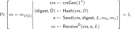
  where the probability is taken over the random choices made by crsGen and Send.

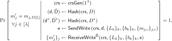
• Correctness of Writes: For any database D of size at most $\textsf {poly} (\lambda )$ for any polynomial function $\textsf {poly} (\cdot )$, any M memory locations $\{L_j\}_j \in [|D|]^M$ and any bits $\{b_j\}_j$, and any pairs of messages $\{m_{j, c}\}_{j, c} \in \{0, 1\}^{2\lambda ^2}$, let $D^*$ be the database to be D after making the modifications $D[L_j] \leftarrow b_j$ for $j = 1, ..., M$, we require that

  

  where the probability is taken over the random choices made by crsGen and Send.

• Sender Privacy: There exists a PPT simulator $\ell \textsf {OTSim}$ such that for any non-uniform PPT adversary $\mathcal A = (\mathcal A_1, \mathcal A_2)$ there exists a negligible function $\textsf {negl} (\cdot )$ s.t.

  $$ |\Pr [\textsf {SenPrivExpt} ^{\textsf {real} }(1^\lambda , \mathcal A) = 1] - \Pr [\textsf {SenPrivExpt} ^{\textsf {ideal} }(1^\lambda , \mathcal A) = 1]| \le \textsf {negl} (\lambda ), $$

  where $\textsf {SenPrivExpt} ^{\textsf {real} }$ and $\textsf {SenPrivExpt} ^{\textsf {ideal} }$ are described in Fig. 3.

• Sender Privacy for Writes: There exists a PPT simulator $\ell \textsf {OTSimWrite}$ such that for any non-uniform PPT adversary $\mathcal A = (\mathcal A_1, \mathcal A_2)$ there exists a negligible function $\textsf {negl} (\cdot )$ s.t.

  $$\begin{aligned} |\Pr [\textsf {SenPrivWriteExpt} ^{\textsf {real} }(1^\lambda , \mathcal A) = 1] - \Pr [\textsf {SenPrivWriteExpt} ^{\textsf {ideal} }(1^\lambda , \mathcal A) = 1]| \le \textsf {negl} (\lambda ), \end{aligned}$$

  where $\textsf {SenPrivWriteExpt} ^{\textsf {real} }$ and $\textsf {SenPrivWriteExpt} ^{\textsf {ideal} }$ are described in Fig. 4.

• Efficiency: The algorithm Hash runs in time $|D|\textsf {poly} (\log |D|, \lambda )$. The algorithms Send, Receive run in time $\textsf {poly} (\log |D|, \lambda )$, and the algorithms SendWrite, ReceiveWrite run in time $M \cdot \textsf {poly} (\log |D|, \lambda )$.

Fig. 4.

Sender privacy security game for writes

It is also helpful to introduce the $\ell OT$ scheme with factor-2 compression, which is used in $\ell OT$’s original construction [CDG+17].

Definition 3

An $\ell OT$ scheme with factor-2 compression $\ell OT_{\textsf {const} }$ is an $\ell OT$ scheme where the database D has to be of size $2\lambda$.

Remark 1

The sender privacy requirement here is from [GS18]. It requires crs to be given to the adversary before the adversary chooses his challenge instead of after, and is therefore stronger than the original security requirement [CDG+17]. But we note that in the security proof of laconic oblivious transfer, such adaptive security requirement can be directly reduced to adaptive security for $\ell OT_{\textsf {const} }$. And in the construction of [CDG+17], in every hybrid, crs is generated either truthfully, or generated statistically binding to one of $2\lambda$ possible positions. Therefore, we will incur at most a $1/2\lambda$ loss in the security reduction, simply by guessing which position we need to bind to in those hybrids. This also applies to the sender privacy for parallel writes we will discuss later.

Theorem 4

([CDG+17, DG17, BLSV18, DGHM18]). Assuming either the Computational Diffie-Hellman assumption or the Factoring assumption or the Learning with Errors assumption, there exists a construction of laconic oblivious transfer.

4 Adaptive Garbled Circuits Preserving Parallel Runtime

In this section, we construct an adaptively secure garbling scheme for circuits that allows for parallel evaluation without compromising near-optimal online complexity. We follow the definition of adaptive garbled circuits from [HJO+16].

Definition 4

An adaptive garbling scheme for circuits is a tuple of PPT algorithms

$(\textsf {AdaGCircuit} , \textsf {AdaGInput} , \textsf {AdaEval} )$ such that:

• $(\tilde{C}, \textsf {st} ) \leftarrow \textsf {AdaGCircuit} \left( 1^\lambda , C\right)$. It takes as input a security parameter $\lambda$, a circuit $C: \{0, 1\}^n \mapsto \{0, 1\}^m$ and outputs a garbled circuit $\tilde{C}$ and state information st.

• $\tilde{x} \leftarrow \textsf {AdaGInput} (\textsf {st} , x)$: It takes as input the state information st and an input $x \in \{0, 1\}^n$ and outputs the garbled input $\tilde{x}$.

• $y \leftarrow \textsf {AdaEval} (\tilde{C}, \tilde{x})$. Given a garbled circuit $\tilde{\textsf {C} }$ and a garbled input $\tilde{x}$, AdaEval outputs $y \in \{0, 1\}^m$.

Correctness. For any $\lambda \in \mathbf N$ circuit $\textsf {C} : \{0, 1\}^n \mapsto \{0, 1\}^m$ and input $x \in \{0, 1\}^n$, we have that

$$ \Pr \left[ C(x) = \textsf {AdaEval} (\tilde{C}, \tilde{x})\right] = 1, $$

where $(\tilde{C}, \textsf {st} ) \leftarrow \textsf {AdaGCircuit} \left( 1^\lambda , C\right)$ and $\tilde{x} \leftarrow \textsf {AdaGInput} (\textsf {st} , x)$.

Adaptive Security. There is a PPT simulator $\textsf {AdaGSim} = (\textsf {AdaGSimC} , \textsf {AdaGSimIn} )$ such that, for any non-uniform PPT adversary $\mathcal A = (\mathcal A_1, \mathcal A_2, \mathcal A_3)$ there exists a negligible function $\textsf {negl} (\cdot )$ such that

$$ |\Pr [\textsf {AdaGCExpt} ^{\textsf {real} }(1^\lambda , \mathcal A) = 1] - \Pr [\textsf {AdaGCExpt} ^{\textsf {ideal} }(1^\lambda , \mathcal A) = 1]| \le \textsf {negl} (\lambda ), $$

where $\textsf {AdaGCExpt} ^{\textsf {real} }$ and $\textsf {AdaGCExpt} ^{\textsf {ideal} }$ are described in Fig. 5.

Online Complexity. The running time of AdaGInput is called the online computational complexity and $|\tilde{x}|$ is called the online communication complexity. We require that the online computational complexity does not scale linearly with the size of the circuit |C|.

Furthermore, we call the garbling scheme is parallelly efficient, if the algorithms are given as probabilistic PRAM programs with M processors, and the parallel runtime of AdaGCircuit is $\textsf {poly} (\lambda ) \cdot |C|/M$ if $|C| \ge M$, the parallel runtime of AdaGInput on a PRAM machine to be $n/M \cdot \textsf {poly} (\lambda , \log |C|)$, and the parallel runtime of AdaEval is $\textsf {poly} (\lambda ) \cdot d$ if $M \ge w$, where w, d is the width and depth of the circuit respectively.

Fig. 5.

Adaptive security game of adaptive garble circuits

4.1 Construction Overview

First, we recall the construction of [GS18], which we will use as a starting point. At a high level, their construction can be viewed as a “weak” garbling of a special RAM program that evaluates the circuit.

In the ungarbled world, a database D is used as RAM to store all the wires (including input, output, and intermediate wires). Initially, D only holds the input and everything else is uninitialized. In each iteration, the processor takes a gate, read two bits according to the gate, evaluate the gate, and write the output bit back into the database. Finally, after all iterations are finished, the output of the circuit is read from the database.

In the garbled world, the database D will be hashed as $\hat{D}$ using $\ell OT$ and protected with an one-time pad r as $\ell OT$ does not protect its memory content. The evaluation process is carried out by a sequence of Yao’s garbled circuits and laconic OT “talking” to each other. In each iteration, two read operations correspond to a selectively secure garbled circuit, which on given digest as input, outputs two $\ell OT$ read ciphertexts that the evaluator can decrypt to the input label for the garbled gate, which is a selectively secure garbled circuit that unmasks the input, evaluates the gate, and then unmasks the output. To store the output, the garbled gate generates a $\ell OT$ block-write ciphertext, which also enables the evaluator to obtain the input labels for the updated digest in the next iteration. This garbled RAM program is then encrypted using a somewhere equivocal encryption, after which it is given to the adversary as the garbled circuit. On given input x, we generate the protected database $\hat{D}$ and compute the input labels for the initial digest, and we give out the labels, the masked input, the decryption key, and masks for output in the database.

This garbling is weak as in it only concerns a particular RAM program, and it does not protect the memory access pattern, but it is sufficient for the adaptive security requirement of garbled circuits as the pattern is fixed and public. As we will see in the security proof that online complexity is tightly related to the pebbling complexity of a pebbling game. The pebbling game is played on a simulation dependency graph, where pieces of garbled circuits in the construction correspond to nodes and hardwiring of input labels correspond to edges. As the input labels for every selectively secure circuit is only hardcoded in the previous circuit, the simulation dependency is a line and there is a known good pebbling strategy.

To parallelize this construction, we naturally wish to evaluate M gates in parallel using a PRAM program instead of evaluating sequentially. This way, we preserve its mostly linear structure, for which we know a good pebbling strategy. Reading from the database is inherently parallelizable, but writing is more problematic as the processors need to communicate with each other to compute the updated digest and we need to be more careful.

4.2 Block-Writing Laconic OT

Recall from Sect. 2.1 that we cannot hope to use $\ell OT$ as a black box in parallel, thus we first briefly recall the techniques used in [CDG+17] to bootstrap an $\ell OT$ scheme with factor-2 compression $\ell OT_{\textsf {const} }$ into a general $\ell OT$ scheme with an arbitrary compression factor.

Consider a database D with size $|D| = 2^d \cdot \lambda$. In order to obtain a hash function with arbitrary (polynomial) compression factor, it’s natural to use a Merkle tree to compress the database. The Hash function outputs $(\textsf {digest} , \hat{\textsf {D} })$, where $\hat{\textsf {D} }$ is the Merkle tree and digest is the root of the tree. Using $\ell OT_{\textsf {const} }$ combined with a Merkle tree, the sender is able to traverse down the Merkle tree, simply by using $\ell OT_{\textsf {const} }.\textsf {Send}$ to obtain the digest for any child he wishes to, until he reaches the block he would like to query. For writes, the sender can read out all the relevant neighbouring digests from the Merkle tree and compute the updated digest using the information. In order to compress the round complexity down to 1 from d, we can use Yao’s garble circuit to garble $\ell OT_{\textsf {const} }.\textsf {Send}$ so that the receiver can evaluate it for the sender, until he gets the final output. On a high level, the receiver makes the garbled circuits and $\ell OT_{\textsf {const} }$ talk to each other to evaluate the read/write ciphertexts.

As mentioned in Sect. 2.1, we wish to construct a block-write procedure such that the following holds:

• The parallel running time should be $\textsf {poly} (\lambda , \log |C|)$;

• For near-optimal online complexity, both the size of each piece of the garbled circuit and the pebbling complexity needs to be $\textsf {poly} (\lambda , \log |C|)$.

Note that changing the ciphertext to contain all M bits directly do not work in this context, as now the write ciphertext would be of length $\Omega (M)$, therefore the garbled circuit generating it must be of length $\Omega (M)$, which violates what we wish to have. The way to fix this is to instead let the ciphertext only hold the digest of the sub-tree, and the block write ciphertext simply needs to perform a “partial” write to obtain the updated digest, therefore its size is no larger than an ordinary write ciphertext. As it turns out, a tree-like structure in the simulation dependency graph also has good pebbling complexity and we can obtain the sub-tree digest using what we call a garbled Merkle tree, which we will construct in the next section. This way, we resolve all the issues.

Now, we first direct our attention back to constructing block-writes. Formally, we will construct two additional algorithms for updatable laconic oblivious transfer that handles a special case of parallel writes. As we will see later, these algorithms can be used to simplify the construction of adaptive garbled circuit.

• $\textsf {e} _{\textsf {w} } \leftarrow \textsf {SendWriteBlock} \left( \textsf {crs} , \textsf {digest} , L, \textsf {d} , \{m_{j, c}\}_{j \in [\lambda ], c \in \{0, 1\}}\right)$. It takes as input the common reference string crs, a digest digest, a location prefix $L \in \{0, 1\}^P$ with length $P \le \log |D|$ and the digest of the subtree d to be written to location L00...0, L00...1, ..., L11...1, and $\lambda$ pairs of messages $\{m_{j, c}\}_{j \in [\lambda ], c \in \{0, 1\}}$, where each $m_{j, c}$ is of length $\lambda$. It outputs a ciphertext $\textsf {e} _{\textsf {w} }$.

• $\{m_j\}_{j \in [\lambda ]} \leftarrow \textsf {ReceiveWriteBlock} ^{\tilde{\textsf {D} }}(\textsf {crs} , L, \{b_k\}_{k \in [2^M]}, \textsf {e} _{\textsf {w} })$. This is a RAM algorithm with random read/write access to $\tilde{\textsf {D} }$. It takes as input the common reference string crs, M locations $\{L_k\}_{k \in [M]}$ and bits to be written $\{b_k\}_{k \in [M]}$ and a ciphertext $\textsf {e} _{\textsf {w} }$. It updates the state $\tilde{\textsf {D} }$ (such that $D[L_k] = b_k$ for every $k \in [M]$) and outputs messages $\{m_j\}_{j \in [\lambda ]}$.

The formal construction of block-writing $\ell OT$ is as follows:

• $\textsf {SendWriteBlock} \left( \textsf {crs} , \textsf {digest} , L, \textsf {d} , \{m_{j, c}\}_{j \in [\lambda ], c \in \{0, 1\}}\right)$

  • Reinterpret the $\ell OT$ Merkle tree by truncating at the |L|-th layer

  • Output $\ell OT.\textsf {SendWrite} \left( \textsf {crs} , \textsf {digest} , L, \textsf {d} , \{m_{j, c}\}_{j \in [\lambda ], c \in \{0, 1\}}\right)$

• $\textsf {ReceiveWriteBlock} ^{\tilde{\textsf {D} }}(\textsf {crs} , L, \{b_k\}_{k \in [2^M]}, \textsf {e} _{\textsf {w} })$

  • Compute the digest d of database $\{b_k\}_{k \in [2^M]}$

  • Reinterpret the $\ell OT$ Merkle tree by truncating at the |L|-th layer and $\tilde{\textsf {D} }$ as the corresponding truncated version of the database

  • $\textsf {Label} \leftarrow \ell OT.\textsf {ReceiveWrite} ^{\tilde{\textsf {D} }}(\textsf {crs} , L, \{b_k\}_{k \in [2^M]}, \textsf {e} _{\textsf {w} })$

  • Update $\tilde{\textsf {D} }$ at block location L using data $\{b_k\}_{k \in [2^M]}$

  • Output $\textsf {Label}$

Fig. 6.

Block-writing security simulator

We require similar security and efficiency requirements for block-writing $\ell OT$. It’s not hard to see that the update part of ReceiveWriteBlock can be evaluated efficiently in parallel (and the call to normal $\textsf {ReceiveWrite}$ only needs to run once), and the security proof can be easily reduced to that of SendWrite, and the security simulator is given in Fig. 6.

4.3 Garbled Merkle Tree

We will now describe an algorithm called garbled Merkle tree. Roughly speaking, a garbled Merkle tree is a binary tree of garbled circuits, where each of the circuit takes arbitrary $2\lambda$ bits as input and outputs the labels of $\lambda$ bit digest. Looking ahead, this construction allows for exponentially smaller online complexity compared to simply garbling the entire hash circuit when combined with adaptive garbling schemes we will construct later, since its tree structure allows for small pebbling complexity.

A garbled Merkle tree has very similar syntax as the one for garbled circuit. It consists of 2 following PPT algorithms:

Fig. 7.

Hashing sub-circuit

• $\textsf {GHash} (1^\lambda , H, \{\textsf {Key} _i\}_{i \in [|D|]}, \{\textsf {Key} '_i\}_{i \in [\lambda ]})$: it takes as input a security parameter $\lambda$, a hashing circuit H that takes $2\lambda$ bits as input and outputs $\lambda$ bits, keys $\{\textsf {Key} _i\}_{i \in [|D|]}$ for all bits in the database D and $\{\textsf {Key} '_i\}_{i \in [\lambda ]}$ for all output bits

  • $\textsf {Keys} _1 \leftarrow \{\textsf {Key} '_i\}_{i \in [\lambda ]}$

  • Sample $\{\textsf {Keys} _i\}_{i = 2, ..., |D|/\lambda - 1}$

  • $\{\textsf {Keys} _i\}_{i = |D|/\lambda , ..., 2|D|/\lambda - 1} \leftarrow \{\textsf {Key} _i\}_{i \in [|D|]}$

  • For $i = 1$ to $|D|/\lambda - 1$ do

       $\tilde{C}_i \leftarrow \textsf {GCircuit} (1^\lambda , \textsf {C} [H, \textsf {Keys} _i], (\textsf {Keys} _{2i}, \textsf {Keys} _{2i + 1}))$

  • Output $\{\tilde{C}_i\}_{i \in [|D|/\lambda - 1]}$

  • The circuit C here is given in Fig. 7.

• $\textsf {GHEval} \left( \{\tilde{C}_i\}, \{\textsf {lab} _i\}_{i \in [|D|]}\right)$: it takes as input the garbled circuits $\{\tilde{C}_i\}_{i \in [|D|/\lambda - 1]}$ and input labels for the database $\{\textsf {lab} _i\}_{i \in [|D|]}$

  • $\{\textsf {Label} _i\}_{i = |D|/\lambda , ..., 2|D|/\lambda - 1} \leftarrow \{\textsf {lab} _i\}_{i \in [|D|]}$

  • For $i = |D|/\lambda - 1$ down to 1 do

       $\textsf {Label} _i \leftarrow \textsf {GCEval} (\tilde{C}_i, (\textsf {Label} _{2i}, \textsf {Label} _{2i + 1}))$

  • Output $\textsf {Label} _1$

Later, we will also invoke this algorithm in garbled PRAM for creating parallel checkpoints.

4.4 Construction

We will now give the construction of our adaptive garbled circuits. Let $\ell OT$ be a laconic oblivious transfer scheme, $(\textsf {GCircuit} , \textsf {GCEval} )$ be a garbling scheme for circuits, $(\textsf {GHash} , \textsf {GHEval} )$ be a garbling scheme for Merkle trees, and $\textsf {SEE}$ be a somewhere equivocal encryption scheme with block length $\textsf {poly} (\lambda , \log |C|)$ to be the maximum size of garbled circuits $\left\{ \widetilde{\textsf {C} }_{i, k}^{\textsf {eval} }, \widetilde{\textsf {C} }_{i, j}^{\textsf {hash} }, \widetilde{\textsf {C} }_i^{\textsf {write} }\right\}$, message length $2M\ell = O(|C|^2)$ (we will explain $\ell$ shortly after) and equivocation parameter $\log \ell + 2 \log M + O(1)$ (the choice comes from the security proof).

Furthermore, we assume both M and $\lambda$ is a power of 2 and $\lambda$ divides M. We also have a procedure $\{P_i\}_{i \in [\ell ]} \leftarrow \textsf {Partition} (C, M)$ (as an oracle) that partition the circuit’s wires 1, 2, ..., |C| into $\ell$ continuous partitions of size M, such that for any partition $P_i$, its size is at most M (allowing a few extra auxiliary wires and renumbering wires), and every gate in the partition can be evaluated in parallel once every partition $P_j$ with $j < i$ has been evaluated. Clearly $d \le \ell \le |C|$, but it’s also acceptable to have a sub-optimal partition to best utilize the computational resources on a PRAM machine. We assume the input wires are put in partition 0. This preprocessing is essentially scheduling the evaluation of the circuit to a PRAM machine and it is essential to making our construction’s online complexity small.

We now give an overview of our construction. At a high level, instead of garbling the circuit directly, our construction can be viewed as a garbling of a special PRAM program that evaluates the circuit in parallel. The database D will be hashed as $\hat{D}$ using $\ell OT$ and protected with an one-time pad r as $\ell OT$ does not protect its memory content. In each iteration, two read operations for every processor correspond to two selectively secure garbled circuits, which on given digest as input, outputs a $\ell OT$ read ciphertext that generates the input label for the garbled gate; the garbled gate unmasks the input, evaluates the gate, and then output the masked output of the gate. After all M processors have done evaluating their corresponding gates, a garbled Merkle tree will take their outputs as input to obtain the digest for the M bits of output, and then generate a $\ell OT$ block-write ciphertext to store the outputs into the database. During evaluation, this block-write ciphertext can be used to obtain the input labels for the read circuits in the next iteration. This garbled PRAM program is then encrypted using a somewhere equivocal encryption, after which it is given to the adversary as the garbled circuit. On given input x, we generate the protected database $\hat{D}$ and compute the input labels for the initial digest, and we give out the labels, the masked inputs, the decryption key, and masks for outputs in the database.

Now we formally present the construction (the description of the evaluation circuit used in the construction is given in Fig. 8). Inside the construction, we omit $k \in [M]$ when the context is clear. It might also be helpful to see Fig. 9 for how the garbled circuits are organized.

Fig. 8.

Description of the evaluation circuit

• $\textsf {AdaGCircuit} ^{\textsf {Partition} }\left( 1^\lambda , C\right)$:

  • $\textsf {crs} \leftarrow \ell OT.\textsf {crsGen} (1^\lambda )$

  • $\textsf {key} \leftarrow \textsf {SEE.KeyGen} (1^\lambda )$

  • $K \leftarrow \textsf {PRFKeyGen} (1^\lambda )$

  • $\{P_i\}_{i \in [\ell ]} \leftarrow \textsf {Partition} (C)$

  • Sample $r \leftarrow \{0, 1\}^{M\ell }$

  • For $i = 1$ to $\ell$ do:

        Let $C_{g, 1}, C_{g, 2}$ denote the two input gates of gate g

        $\begin{aligned} \widetilde{\textsf {C} }_{i, k}^{\textsf {eval} } \leftarrow \textsf {GCircuit} (&1^\lambda , \textsf {C} _{\textsf {eval} }^{\textsf {real} }[\textsf {crs} , C_{P_{i, k}, 1}, C_{P_{i, k}, 2}, P_{i, k}, (r_{C_{P_{i, k}, 1}}, r_{C_{P_{i, k}, 2}}, r_{P_{i, k}}), \\&\quad \quad \quad \textsf {PRF} _K(1, i, k, 0), \textsf {PRF} _K(1, i, k, 1)], \\&\{\textsf {PRF} _K(0, i, j, b)\}_{j \in [\lambda ], b \in \{0, 1\}}) \end{aligned}$

       Let $\textsf {keyEval} = \{\textsf {PRF} _K(1, i, k, b)\}_{k \in [M], b \in \{0, 1\}}$

       Let $\textsf {keyHash} = \{\textsf {PRF} _K(2, i, j, b)\}_{j \in [\lambda ], b \in \{0, 1\}}$

       $\{\widetilde{\textsf {C} }_{i, j}^{\textsf {hash} }\}_{j \in [M - 1]} \leftarrow \textsf {GHash} (1^\lambda , \ell OT_{\textsf {const} }.\textsf {Hash} , \textsf {keyEval} , \textsf {keyHash} )$

       Let $C_i^{\textsf {write} } = \ell OT.\textsf {SendWriteBlock} \left( \textsf {crs} , \cdot , i, \{\textsf {PRF} _K(0, i + 1, j, b)\}_{j \in [\lambda ], b \in \{0, 1\}}\right)$

       $\widetilde{\textsf {C} }_i^{\textsf {write} } \leftarrow \textsf {GCircuit} \left( 1^\lambda , C_i^{\textsf {write} }, \textsf {keyHash} \right)$

  • $c \leftarrow \textsf {SEE.Enc} \left( \textsf {key} , \left\{ \widetilde{\textsf {C} }_{i, k}^{\textsf {eval} }, \widetilde{\textsf {C} }_{i, j}^{\textsf {hash} }, \widetilde{\textsf {C} }_i^{\textsf {write} }\right\} \right)$

  • Output $\tilde{C} := (\textsf {crs} , c, \{P_i\}_{i \in [\ell ]})$ and $\textsf {st} := (\textsf {crs} , r, \textsf {key} , \ell , K)$

• $\textsf {AdaGInput} (\textsf {st} , x)$:

  • Parse $\textsf {st} := (\textsf {crs} , r, \textsf {key} , \ell , K)$

  • $D \leftarrow r_1 \oplus x_1 || ... || r_n \oplus x_n || 0^{M\ell - n}$

  • $(\textsf {d} , \hat{D}) \leftarrow \ell OT.\textsf {Hash} (\textsf {crs} , D)$

  • Output $(\{\textsf {PRF} _K(0, 1, j, \textsf {d} _j)\}_{j \in [\lambda ]}, r_1 \oplus x_1 || ... || r_n \oplus x_n, \textsf {key} , r_{N - m + 1} || ... || r_N)$

• $\textsf {AdaEval} (\tilde{C}, \tilde{x})$:

  • Parse $\tilde{C} := (\textsf {crs} , c, \{P_i\}_{i \in [\ell ]})$

  • Parse $\tilde{x} := (\{\textsf {lab} _{0, j}\}_{j \in [\lambda ]}, s_1 || ... || s_n, \textsf {key} , r_{N - m + 1} || ... || r_N)$

  • $D \leftarrow s_1 || ... || s_n || 0^{M\ell - n}$

  • $(\textsf {d} , \hat{D}) \leftarrow \ell OT.\textsf {Hash} (\textsf {crs} , D)$

  • $\left\{ \widetilde{\textsf {C} }_{i, k}^{\textsf {eval} }, \widetilde{\textsf {C} }_{i, j}^{\textsf {hash} }, \widetilde{\textsf {C} }_i^{\textsf {write} }\right\} \leftarrow \textsf {SEE.Dec} (\textsf {key} , c)$

  • For $i = 1$ to $\ell$ do:

        Let $C_{g, 1}, C_{g, 2}$ denote the two input gates of gate g

       $\textsf {e} \leftarrow \textsf {GCEval} (\widetilde{\textsf {C} }_{i, k}^{\textsf {eval} }, \{\textsf {lab} _{0, j}\}_{j \in [\lambda ]})$

       $\textsf {e} \leftarrow \ell OT.\textsf {Receive} ^{\hat{D}}(\textsf {crs} , \textsf {e} , C_{P_{i, k}, 1})$

       $(\gamma _k, \textsf {lab} _{1, k}) \leftarrow \ell OT.\textsf {Receive} ^{\hat{D}}(\textsf {crs} , \textsf {e} , C_{P_{i, k}, 2})$

       $\{\textsf {lab} _{2, j}\}_{j \in [\lambda ]} \leftarrow \textsf {GHEval} (\{\widetilde{\textsf {C} }_{i, j}^{\textsf {hash} }\}_{j \in [M - 1]}, \{\textsf {lab} _{1, k}\}_{k \in [M]})$

       $\textsf {e} \leftarrow \textsf {GCEval} (\widetilde{\textsf {C} }_i^{\textsf {write} }, \{\textsf {lab} _{2, j}\}_{j \in [\lambda ]})$

       $\{\textsf {lab} _{0, j}\}_{j \in [\lambda ]} \leftarrow \ell OT.\textsf {ReceiveWriteBlock} ^{\tilde{\textsf {D} }}(\textsf {crs} , i, \{\gamma _k\}_{k \in [M]}, \textsf {e} )$

  • Recover the contents of the memory D from the final state $\hat{D}$

  • Output $D_{N - m + 1} \oplus r_{N - m + 1} || ... || D_N \oplus r_N$

Fig. 9.

Illustration of the pebbling graph for one layer: $\widetilde{\textsf {C} }_{i, k}^{\textsf {eval} }$ are leaf nodes, $\widetilde{\textsf {C} }_{i, j}^{\textsf {hash} }$ are intermediate nodes and the root node, finally $\widetilde{\textsf {C} }_i^{\textsf {write} }$ is the extra node at the end. Dotted edges indicate where $\ell OT$ is invoked. Note that WriteBlock is only invoked once and its result is reused M times.

Communcation Complexity of AdaGInput. It follows from the construction that the communication complexity of AdaGInput is $\lambda ^2 + n + m + |\textsf {key} |$. From the parameters used in the somewhere equivocal encryption and the efficiency of block writing for laconic oblivious transfer, we note that $|\textsf {key} | = \textsf {poly} (\lambda , \log |C|)$.

Computational Complexity of AdaGInput. The running time of AdaGInput grows linearly with |C|. However, it’s possible to delegate the hashing of zeros to the offline phase, i.e. AdaGCircuit. In that case, the running time only grows linearly with $n + \log |C|$.

Parallel Efficiency. With a good Partition algorithm and number of processors as many as the width of the circuit, AdaEval is able to run in $d \cdot \textsf {poly} (\lambda , \log |C|)$ where d is the depth of the circuit.

Correctness. We note that for each wire (up to permutation due to rewiring), our construction manipulates the database and produces the final output the same way as the construction given by [GS18]. Therefore by the correctness of their construction, our construction outputs C(x) with probability 1.

Adaptive Security. We formally prove the adaptive security in the full version.

References

Ananth, P., Chen, Y.-C., Chung, K.-M., Lin, H., Lin, W.-K.: Delegating RAM computations with adaptive soundness and privacy. In: Hirt, M., Smith, A. (eds.) TCC 2016. LNCS, vol. 9986, pp. 3–30. Springer, Heidelberg (2016). https://doi.org/10.1007/978-3-662-53644-5_1
Ajtai, M., Komlós, J., Szemerédi, E.: An O(n log n) sorting network. In: Proceedings of the Fifteenth Annual ACM Symposium on Theory of Computing, STOC 1983, pp. 1–9. ACM, New York (1983)
Applebaum, B.: Garbled circuits as randomized encodings of functions: a primer. In: Lindell, Y. (ed.) Tutorials on the Foundations of Cryptography. ISC, pp. 1–44. Springer, Cham (2017). https://doi.org/10.1007/978-3-319-57048-8_1
Boyle, E., Chung, K.-M., Pass, R.: Oblivious parallel RAM and applications. In: Kushilevitz, E., Malkin, T. (eds.) TCC 2016. LNCS, vol. 9563, pp. 175–204. Springer, Heidelberg (2016). https://doi.org/10.1007/978-3-662-49099-0_7
Bennett, C.H.: Time/space trade-offs for reversible computation. SIAM J. Comput. 18(4), 766–776 (1989)
Bellare, M., Hoang, V.T., Rogaway, P.: Adaptively secure garbling with applications to one-time programs and secure outsourcing. In: Wang, X., Sako, K. (eds.) ASIACRYPT 2012. LNCS, vol. 7658, pp. 134–153. Springer, Heidelberg (2012). https://doi.org/10.1007/978-3-642-34961-4_10
Bellare, M., Hoang, V.T., Rogaway, P.: Foundations of garbled circuits. In: Proceedings of the 2012 ACM Conference on Computer and Communications Security, pp. 784–796. ACM (2012)
Brakerski, Z., Lombardi, A., Segev, G., Vaikuntanathan, V.: Anonymous IBE, leakage resilience and circular security from new assumptions. In: Nielsen, J.B., Rijmen, V. (eds.) EUROCRYPT 2018. LNCS, vol. 10820, pp. 535–564. Springer, Cham (2018). https://doi.org/10.1007/978-3-319-78381-9_20
Chen, Y.-C., Chow, S.S.M., Chung, K.-M., Lai, R.W.F., Lin, W.-K., Zhou, H.-S.: Cryptography for parallel RAM from indistinguishability obfuscation. In: Proceedings of the 2016 ACM Conference on Innovations in Theoretical Computer Science, pp. 179–190. ACM (2016)
Canetti, R., Chen, Y., Holmgren, J., Raykova, M.: Adaptive succinct garbled RAM or: how to delegate your database. In: Hirt, M., Smith, A. (eds.) TCC 2016. LNCS, vol. 9986, pp. 61–90. Springer, Heidelberg (2016). https://doi.org/10.1007/978-3-662-53644-5_3
Cho, C., Döttling, N., Garg, S., Gupta, D., Miao, P., Polychroniadou, A.: Laconic oblivious transfer and its applications. In: Katz, J., Shacham, H. (eds.) CRYPTO 2017. LNCS, vol. 10402, pp. 33–65. Springer, Cham (2017). https://doi.org/10.1007/978-3-319-63715-0_2
Canetti, R., Holmgren, J.: Fully succinct garbled RAM. In: Proceedings of the 2016 ACM Conference on Innovations in Theoretical Computer Science, pp. 169–178. ACM (2016)
Döttling, N., Garg, S.: Identity-based encryption from the Diffie-Hellman assumption. In: Katz, J., Shacham, H. (eds.) CRYPTO 2017. LNCS, vol. 10401, pp. 537–569. Springer, Cham (2017). https://doi.org/10.1007/978-3-319-63688-7_18
Döttling, N., Garg, S., Hajiabadi, M., Masny, D.: New constructions of identity-based and key-dependent message secure encryption schemes. In: Abdalla, M., Dahab, R. (eds.) PKC 2018. LNCS, vol. 10769, pp. 3–31. Springer, Cham (2018). https://doi.org/10.1007/978-3-319-76578-5_1
Garg, S., Gupta, D., Miao, P., Pandey, O.: Secure multiparty RAM computation in constant rounds. In: Hirt, M., Smith, A. (eds.) TCC 2016. LNCS, vol. 9985, pp. 491–520. Springer, Heidelberg (2016). https://doi.org/10.1007/978-3-662-53641-4_19
Gentry, C., Halevi, S., Lu, S., Ostrovsky, R., Raykova, M., Wichs, D.: Garbled RAM revisited. In: Nguyen, P.Q., Oswald, E. (eds.) EUROCRYPT 2014. LNCS, vol. 8441, pp. 405–422. Springer, Heidelberg (2014). https://doi.org/10.1007/978-3-642-55220-5_23
Garg, S., Lu, S., Ostrovsky, R.: Black-box garbled RAM. In: 2015 IEEE 56th Annual Symposium on Foundations of Computer Science (FOCS), pp. 210–229. IEEE (2015)
Garg, S., Lu, S., Ostrovsky, R., Scafuro, A.: Garbled RAM from one-way functions. In: Proceedings of the Forty-Seventh Annual ACM Symposium on Theory of Computing, pp. 449–458. ACM (2015)
Garg, S., Ostrovsky, R., Srinivasan, A.: Adaptive garbled RAM from laconic oblivious transfer. In: Shacham, H., Boldyreva, A. (eds.) CRYPTO 2018. LNCS, vol. 10993, pp. 515–544. Springer, Cham (2018). https://doi.org/10.1007/978-3-319-96878-0_18
Garg, S., Srinivasan, A.: Adaptively secure garbling with near optimal online complexity. In: Nielsen, J.B., Rijmen, V. (eds.) EUROCRYPT 2018. LNCS, vol. 10821, pp. 535–565. Springer, Cham (2018). https://doi.org/10.1007/978-3-319-78375-8_18
Hemenway, B., Jafargholi, Z., Ostrovsky, R., Scafuro, A., Wichs, D.: Adaptively secure garbled circuits from one-way functions. In: Robshaw, M., Katz, J. (eds.) CRYPTO 2016. LNCS, vol. 9816, pp. 149–178. Springer, Heidelberg (2016). https://doi.org/10.1007/978-3-662-53015-3_6
Jafargholi, Z., Kamath, C., Klein, K., Komargodski, I., Pietrzak, K., Wichs, D.: Be adaptive, avoid overcommitting. In: Katz, J., Shacham, H. (eds.) CRYPTO 2017. LNCS, vol. 10401, pp. 133–163. Springer, Cham (2017). https://doi.org/10.1007/978-3-319-63688-7_5
Jafargholi, Z., Scafuro, A., Wichs, D.: Adaptively indistinguishable garbled circuits. In: Kalai, Y., Reyzin, L. (eds.) TCC 2017. LNCS, vol. 10678, pp. 40–71. Springer, Cham (2017). https://doi.org/10.1007/978-3-319-70503-3_2
Jafargholi, Z., Wichs, D.: Adaptive security of Yao’s garbled circuits. In: Hirt, M., Smith, A. (eds.) TCC 2016. LNCS, vol. 9985, pp. 433–458. Springer, Heidelberg (2016). https://doi.org/10.1007/978-3-662-53641-4_17
Lu, S., Ostrovsky, R.: How to garble RAM programs? In: Johansson, T., Nguyen, P.Q. (eds.) EUROCRYPT 2013. LNCS, vol. 7881, pp. 719–734. Springer, Heidelberg (2013). https://doi.org/10.1007/978-3-642-38348-9_42
Lu, S., Ostrovsky, R.: Black-box parallel garbled RAM. In: Katz, J., Shacham, H. (eds.) CRYPTO 2017. LNCS, vol. 10402, pp. 66–92. Springer, Cham (2017). https://doi.org/10.1007/978-3-319-63715-0_3
Paul, W.J., Tarjan, R.E., Celoni, J.R.: Space bounds for a game on graphs. Math. Syst. Theory 10(1), 239–251 (1976)
Yao, A.C.: Protocols for secure computations. In: 23rd Annual Symposium on Foundations of Computer Science, 1982, SFCS’08, pp. 160–164. IEEE (1982)
Acknowledgements
The authors would like to thank Tsung-Hsuan Hung and Yu-Chi Chen for their helpful discussions in the early stage of this research.
Author information
Authors and Affiliations
Corresponding author
Editor information
Editors and Affiliations
Rights and permissions
Copyright information
© 2019 International Association for Cryptologic Research
About this paper
Cite this paper
Chung, KM., Qian, L. (2019). Adaptively Secure Garbling Schemes for Parallel Computations. In: Hofheinz, D., Rosen, A. (eds) Theory of Cryptography. TCC 2019. Lecture Notes in Computer Science(), vol 11892. Springer, Cham. https://doi.org/10.1007/978-3-030-36033-7_11
Download citation
DOI: https://doi.org/10.1007/978-3-030-36033-7_11
Published:
Publisher Name: Springer, Cham
Print ISBN: 978-3-030-36032-0
Online ISBN: 978-3-030-36033-7
eBook Packages: Computer ScienceComputer Science (R0)