Incrementally Verifiable Computation via Incremental PCPs

Abstract

If I commission a long computation, how can I check that the result is correct without re-doing the computation myself? This is the question that efficient verifiable computation deals with. In this work, we address the issue of verifying the computation as it unfolds. That is, at any intermediate point in the computation, I would like to see a proof that the current state is correct. Ideally, these proofs should be short, non-interactive, and easy to verify. In addition, the proof at each step should be generated efficiently by updating the previous proof, without recomputing the entire proof from scratch. This notion, known as incrementally verifiable computation, was introduced by Valiant [TCC 08] about a decade ago. Existing solutions follow the approach of recursive proof composition and can be based on strong and non-falsifiable cryptographic assumptions (so-called “knowledge assumptions”).

In this work, we present a new framework for constructing incrementally verifiable computation schemes in both the publicly verifiable and designated-verifier settings. Our designated-verifier scheme is based on somewhat homomorphic encryption (which can be based on Learning with Errors) and our publicly verifiable scheme is based on the notion of zero-testable homomorphic encryption, which can be constructed from ideal multi-linear maps [Paneth and Rothblum, TCC 17].

Our framework is anchored around the new notion of a probabilistically checkable proof (PCP) with incremental local updates. An incrementally updatable PCP proves the correctness of an ongoing computation, where after each computation step, the value of every symbol can be updated locally without reading any other symbol. This update results in a new PCP for the correctness of the next step in the computation. Our primary technical contribution is constructing such an incrementally updatable PCP. We show how to combine updatable PCPs with recently suggested (ordinary) verifiable computation to obtain our results.

M. Naor—Supported in part by grant from the Israel Science Foundation (no. 950/16). Incumbent of the Judith Kleeman Professorial Chair.

O. Paneth—Supported by NSF Grants CNS-1413964, CNS-1350619 and CNS-1414119, and the Defense Advanced Research Projects Agency (DARPA) and the U.S. Army Research Office under contracts W911NF-15-C-0226 and W911NF-15-C-0236.

G. N. Rothblum—This project has received funding from the European Research Council (ERC) under the European Union’s Horizon 2020 research and innovation programme (grant agreement No. 819702).

1 Introduction

Efficient verification of complex computations is a foundational question in the theory of computation. Recent years have seen exciting progress in the study of this problem, from a rich theory of efficient protocols to concrete implementations and new application domains. In the verifiable computation paradigm, the output of a computation is accompanied by a proof of the result’s correctness. The proof should be efficient to construct (not much more expensive than simply computing the output), and super-efficient to verify (e.g. verification in nearly-linear time).

Incrementally Verifiable Computation. In this work we revisit the question of incrementally verifiable computation, introduced by Valiant [Val08] about a decade ago. To motivate this question, consider the following scenarios:

Intermediate Outputs: Consider a server that executes a long computation for a client. Even before the entire computation terminates, the client may want to obtain intermediate outputs or to audit the server’s progress throughout the computation. This is especially significant in the presence of transient faults that are hard to detect: suppose that the computation is so long that faults are likely to occur eventually. Without a methodology for detecting these faults, then the final output is likely to be wrong.

Transferable Computation: We would like to split a long sequential computation between different parties such that every party performs a small part of the computation and passes it on to the next party. Together with the current state of their computation, parties should include a proof that the computation was performed correctly, not only in the last step, but in its entirety. As a compelling example, consider an extremely long computation that would require all of humanity many generations to complete. We would like every generation to perform its part, and pass the state of the computation along to the next generation together with a proof of correctness.

In both examples above we need a correctness proof that can be constructed incrementally, so that at any intermediate point in the computation, the current state can be verified. The process of updating the proof must be fast and stateless, meaning that, first, the time to update the proof is independent of the running time of the computation so far and, second, to update the proof we only need to know the most recent version of the proof and the current state of the computation.

We restrict our attention to non-interactive protocols for deterministic computations, where both the prover and verifier have access to an honestly generated common reference string, and where soundness is only required to hold against computationally bounded adversarial provers. Even without the issue of incremental updates, both of these relaxations are known to be necessary under standard complexity theoretic assumptions (see Goldreich and Håstad [GH98]).

In a verifiable computation protocol an honest prover executes a program $M$ on input $y$. For every timestep $t$, let $c_t$ denote the state of the program (including the program’s entire memory) after the first $t$ steps. Given the common reference string (CRS) the prover constructs a proof $\varPi _t$ for the correctness of the state $c_t$. For security parameter $\kappa$, the verifier takes the CRS, the input $y$, the state $c_t$ and the proof $\varPi _t$ and decides if to accept the proof in time $(|y|+|c_t|)\cdot \mathrm {poly}(\kappa )$, independently of $t$. Soundness asserts that, given an honestly generated CRS, no efficient adversarial prover can find an input $y$, a time $t$ and an accepting proof for any state other then $c_t$ (except with negligible probability).

A verifiable computation protocol is incrementally updatable if there is an update procedure that, given the CRS, the state $c_t$ and the proof $\varPi _t$, computes the proof $\varPi _{t+1}$ for the next state in time $(|y|+|c_t|)\cdot \mathrm {poly}(\kappa )$.

The State of the Art. Valiant presented an approach for constructing incrementally verifiable computation based on the idea of recursive proof composition. Very roughly, given a proof $\varPi _t$ for state $c_t$ the updated proof $\varPi _{t+1}$ for the next state $c_{t+1}$ asserts that: (1) there exists a state $c_t$ and a proof $\varPi _t$ for timestep $t$ that are accepted by the verifier, and (2) the computation starting from state $c_t$ transitions to state $c_{t+1}$. Constructing the proof $\varPi _{t+1}$ given $c_t$ and $\varPi _t$ may potentially be fast since $\varPi _{t+1}$ only argues about the fast verification algorithm and one step of the computation.

The challenge in implementing this idea is maintaining soundness. Existing solutions are based on the strong notion of succinct non-interactive arguments of knowledge for non-deterministic computations also known as SNARKs [Val08, BCC+17, BCCT13]. Currently such SNARKs are known based on non-standard non-falsifiable assumptions (so-called “knowledge assumptions”). We therefore ask:

Is incrementally verifiable computation possible under standard assumptions?

1.1 This Work

In this work we give a new framework for constructing incrementally verifiable computation. Based on this framework we give new protocols in both the publicly verifiable and designated-verifier settings.

Designated verifier. In the designated-verifier setting the common reference string (CRS) is generated together with a secret key. Only a verifier that holds this secret key can check the proof, and soundness is not guaranteed against parties who know the secret key. In this setting we prove the following:

Theorem 1.1

(informal). Assuming a somewhat-homomorphic encryption scheme for computations of poly-logarithmic degree, there exists a designated-verifier incrementally verifiable computation protocol.

The protocol is based on the (non-incremental) verifiable computation protocol of Kalai et al. [KRR14] with the improvements of Brakerski et al. [BHK17]. Their construction can use any computational private information retrieval (PIR) scheme. To get incremental updates, we rely on the stronger notion of somewhat-homomorphic encryption. Such encryption schemes are known under the Learning with Errors assumption (see Brakerski and Vaikuntanathan and Gentry et al. [BV11, GSW13]).

Public Verification. In a publicly verifiable protocol, the proof can be verified by anyone who knows the CRS, and there is no secret key. In this setting we prove the following:

Theorem 1.2

(informal). Assuming a 3-key zero-testable somewhat homomorphic encryption scheme with correctness for adversarially-generated ciphertexts, there exists a publicly verifiable incrementally verifiable computation protocol.

The protocol is based on the (non-incremental) verifiable computation protocol of Paneth and Rothblum [PR17] and is proven secure under the same assumption as their work. We refer the reader to [PR17] for the definition of the required notion of zero-testable homomorphic encryption. We note, however, that currently, candidates for such homomorphic encryption are only known based on (efficiently falsifiable) assumptions about ideal multilinear maps.

Our framework deviates from the recursive proof composition approach. Instead, our constructions are based on a new type of probabilistically checkable proof (PCP) with incremental local updates.

Incrementally Updatable PCP. In contrast to the setting of verifiable computation, known constructions in the PCP model have proofs that are longer than the computation whose correctness is being proved. Verification, on the other hand, is performed by querying only a small number of locations in the proof, and in running time that is nearly-linear in the input length. Moreover, in the PCP model positive results are known even for non-deterministic computations with unconditional soundness. PCPs allow us to prove that for a non-deterministic program $M$ and input $y$ there exists a witness $w$ that will make $M$ reach state $c_t$ after $t$ steps. The proof $\varPi _t$ is a string of size $\mathrm {poly}(t)$ over some alphabet $\varSigma$ of size $\mathrm {polylog}(t)$ (our setting requires a non-binary alphabet) and verification queries $\mathrm {polylog}(t)$ symbols of the proof achieving negligible soundness error.

In this setting, the question of incremental updates is as follows: given the proof $\varPi _t$ for state $c_t$, and given a state $c_{t+1}$ that follows $c_t$ (for non-deterministic computations, there may be more than one state that follows $c_t$), we would like to update $\varPi _t$ and obtain a new proof $\varPi _{t+1}$ for $c_{t+1}$. We cannot hope for the update time to be independent of $t$ since, given the error-correcting nature of the proof, every proof symbol must change. Instead we require that every symbol of the proof can “self-update” quickly. That is, given the i-th symbol of $\varPi _t$ and the states $c_t$ and $c_{t+1}$ we can compute the i-th symbol of the new proof $\varPi _{t+1}$ in time $(|y|+|c_t|)\cdot \mathrm {polylog}(t)$.

The main technical contribution of this work is a construction of an incrementally updatable PCP. Our construction is based on the classic PCP of Babai, Fortnow, Levin and Szegedy (BFLS) [BFLS91]. We modify their PCP by considering a larger alphabet $\varSigma$ and augmenting every symbol of the original proof with supplemental values that allow the augmented symbol to self-update.

From PCP to Verifiable Computation, Heuristically. Biehl, Meyer and Wetzel [BMW98] suggested a heuristic transformation from PCPs to verifiable computation protocols. We refer to their technique as the hidden query heuristic. Roughly speaking, the idea is to perform the required PCP queries in a manner that does not allow the prover to figure out the query locations. This idea can be implemented by placing random PCP queries in the CRS, encoded using a private information retrieval (PIR) scheme, or, alternatively, encrypted with a homomorphic encryption scheme (where every query is encrypted under a different key). The prover homomorphically evaluates the PCP answers and sends the encrypted results as the proof. The (designated) verifier decrypts the results and checks that the underlying PCP accepts.

We observe that instantiating the hidden query heuristic with a PCP that can be incrementally updated gives a heuristic incrementally verifiable computation protocol. To see this, recall that following the hidden query heuristic, the proof consists of a few PCP symbols encrypted under homomorphic encryption. Since every one of these symbols can self-update, we can homomorphically evaluate the PCP update procedure under the encryption and obtain encryptions of the updated PCP symbols. We note that, while the hidden query heuristic can be implemented with PIR, getting incrementally verifiable computation requires the stronger notion of homomorphic encryption which supports “multi-hop” evaluation. This is because we update the proof by homomorphically evaluating the PCP update procedure over the encrypted PCP answers.

Secure Instantiations. For many years it was not known whether the hidden query technique can be shown to be sound (see Dwork et al. [DLN+00] for the obstacles in proving its soundness, as well as [DNR16] and [DHRW16]). However, recent works give secure instantiations of this heuristic in both the designated-verifier and the publicly verifiable settings. Next, we discuss these instantiations and explain how we turn them into incrementally verifiable computation protocols based on our incrementally updatable PCP.

Starting from the designated-verifiable setting, the works of [KRR13, KRR14, BHK17] prove that the hidden query heuristic is secure, assuming the underlying PCP satisfies a strong form of soundness called no-signaling soundness. Our designated-verifier protocol is based on the no-signaling PCP construction of Brakerski, Holmgren and Kalai (BHK) [BHK17], which in turn is based on the PCP of BFLS with several changes that facilitate the proof of no-signaling soundness. Very roughly, their construction has the following structure:

• 1. Given a program $M$, define an augmented program $\tilde{M}$ that emulates $M$ while encoding each of its states $c_{t}$ with a particular error correcting code.

• 2. The honest prover computes the PCP proof for the augmented program $\tilde{M}$. This proof is essentially the same as in the PCP of BFLS.

• 3. The verifier locally tests the PCP proof. These tests differ significantly from the tests performed by the original BFLS verifier.

To turn this PCP into a verifiable computation protocol, BHK apply the hidden query technique using any PIR scheme.

To achieve incremental updates, we make the following two changes to the BHK protocol: first, we modify the prover to compute the PCP proof for $\tilde{M}$ using our incrementally updatable PCP instead of the PCP of BFLS. Recall that our PCP augments every symbol of the original BFLS proof with supplemental values. Since these supplemental values are only needed to update the proof, the verifier can simply ignore them. Other than that, our verifier is the same as that of BHK. Second, as discussed above, to turn the PCP into an incrementally verifiable computation protocol we use homomorphic encryption instead of PIR. We note that in our PCP the answers can be computed by a polynomial of poly-logarithmic degree and, therefore, somewhat homomorphic encryption is sufficient [Gen09].

We emphasize that while our honest prover is defined differently, the verification procedure of our incrementally verifiable computation is essentially the same as the one in BHK. Therefore, the soundness of our protocol follows directly from the analysis in BHK. Indeed, the focus of this work is on showing that the honest proof can be constructed incrementally. We note that there some minor differences between the BFLS construction that we use and the one used in BHK. However, a careful inspection shows that the analysis in BHK can be easily modified to fit our PCP (see Sect. 2.4 for more detail).

In the publicly verifiable setting, the work of [PR17] gives a verifiable computation protocol based on the hidden query heuristic. While they do not require that the PCP satisfies no-signaling soundness, they need a stronger notion of homomorphic encryption that supports a weak zero-test operation as well as some additional properties. They show that such encryption can be based on ideal multi-linear maps. Similarly to the BHK protocol, in [PR17], the honest prover simply constructs the PCP proof for an augmented program $\tilde{M}$ using the PCP of BFLS. We modify their protocol to use our incrementally updatable PCP instead and use the same verification procedure (ignoring any supplemental values added to the BFLS proof). Therefore, designated-verifiable setting, the soundness of our protocol follows immediately from the proof analysis of [PR17].

On the Locality of Updates. A natural relaxation of incrementally updatable PCP would allow for updating of every proof symbol given the values of a small number of other symbols. PCPs with such local updates may be easier to construct than PCPs with strictly self-updating symbols. Note, however, that in order to go from incrementally updatable PCPs to incrementally verifiable computation following our framework, it is crucial that PCP symbols can self-update. If computing one symbol of the new proof requires the values of even two old symbols, then the number of symbols we need to maintain under every encryption may grow exponentially with the number of updates.

On Strong Soundness. The focus of this work is on constructing PCPs and verifiable computation protocols where the honest proof can be computed incrementally. An intriguing question for future research is to design PCPs and verifiable computation protocols where even an adversarially generated proof can be updated. That is, if an adversary produces an accepting proof for timestep $t$, we can continue updating this proof to get accepting proof for subsequent steps. This strong soundness guarantee is motivated, for example, by the transferable computation scenario described above where multiple mutually distrustful parties incrementally construct the correctness proof.

Our PCP construction does not satisfy this stronger guarantee. Very roughly, the reason is that we augment the standard PCP of BFLS by adding supplemental values encoded into every symbol. These supplemental values are crucial for implementing self-updates, but play no role in the verification of the PCP. In particular, an adversarially generated proof may consist of a good “core PCP” that verifies correctly, together with corrupted supplemental values that would prevent this PCP from updating.

Related Work. In a recent work, Holmgren and Rothblum [HR18] construct designated-verifier argument systems where the prover’s space and time complexity are very close to the time and space needed to perform the computation. While their work does not consider or achieve the notion of incrementally updatable PCPs, there are technical similarities in the way the two PCP systems are constructed. Indeed, they consider a related notion where the prover is given streaming access to the computation’s tableau. In this related model, they can process additions to the tableau in small amortized time. On a technical level, we note that they do not limit the space used by the machine, which leads to significant complications. Further connections between incrementally verifiable computation and argument systems with very efficient provers were explored in [Val08, BCCT13].

In a very recent work (subsequent to ours), Kalai, Paneth and Yang [KPY19] construct a verifiable computation protocol with public verification based on a falsifiable assumption on bilinear groups. While their protocol also relies on the hidden query technique, we do not know how to make it incremental based on our PCP. This is because their protocol also uses a bootstrapping technique (to go from a long CRS to a short CRS) that significantly complicates the prover’s strategy.

Future Directions. We leave open the question of constructing incrementally verifiable computation protocols with strong soundness, where even adversarially generated proofs can be updated as discussed above. Another interesting direction is to explore alternative approaches to incrementally verifiable computation based on standard assumptions. One potential path towards this goal is to implement Valiant’s idea of recursive proof composition, replacing knowledge assumptions with the recent bootstrapping technique of [KPY19]. We emphasize that the approach proposed in this work is not based on recursive proof composition. In particular, our solution can also be applied in the designated-verifier setting, based on the Learning with Errors assumption.

2 Technical Overview

Next we describe our construction of an incrementally updatable PCP. We start by recalling the PCP of BFLS. In Sect. 2.2 we describe our PCP proof string and in Sect. 2.3 we explain how to update it.

2.1 The BFLS Construction

Our construction builds on the PCP of BFLS [BFLS91]. We recall some of the details of that construction.

Setup. For a non-deterministic polynomial-time Turing machine $M$ and input $y\in \left\{ 0,1\right\} ^n$ we construct a proof for the fact that there exists a witness that makes $M$ accepts $y$. As we know from the Cook-Levin Theorem, it is possible to represent $M$’s computation on an input $y$ by a Boolean 3CNF formula $\phi _y$ over $N=\mathrm {poly}(n)$ variables such that $\phi _y$ is satisfiable if and only if there exists a witness that makes $M$ accept $y$. Let $\mathbb {F}$ be a field of size $\varTheta (\log ^2{N})$ and let $\mathbb {H}\subset \mathbb {F}$ be a subset of size $\log (N)$. We set $u\in \mathbb {N}$ such that $|\mathbb {H}|^u= N$ and index the variables of $\phi _y$ by vectors in $\mathbb {H}^u$. Given a witness that makes $M$ accept $y$ we can compute an assignment $X:\mathbb {H}^u\rightarrow \left\{ 0,1\right\}$ that satisfies $\phi _y$.

Arithmetization. The first part of the PCP proof contains the assignment $X$ represented as a multi-variate polynomial ${\tilde{X}}:\mathbb {F}^{u}\rightarrow \mathbb {F}$ of degree at most $(|\mathbb {H}|-1)$ in each variable, that identifies with $X$ on $\mathbb {H}^u$. We also describe the formula $\phi _y$ algebraically as polynomial $\varphi _y:\mathbb {F}^{\ell }\rightarrow \mathbb {F}$ over $\ell = 3(u+1)$ variables, with individual degree $\mathrm {polylog}(N)$. For every 3 variables $\mathbf {h}_1,\mathbf {h}_2,\mathbf {h}_3 \in \mathbb {H}^{u}$ and 3 bits $b_1,b_2,b_3 \in \left\{ 0,1\right\}$, if the formula $\phi _y$ contains the clause:

$$(X(\mathbf {h}_1) = b_1)\vee (X(\mathbf {h}_2) = b_2)\vee (X(\mathbf {h}_3) = b_3),$$

then the polynomial $\varphi _y$ evaluates to 1 on $(\mathbf {h}_1,\mathbf {h}_2,\mathbf {h}_3,b_1,b_2,b_3)$. Otherwise, $\varphi _y$ evaluates to 0. The polynomial $\varphi _y$ can be computed by an arithmetic circuit of size $\mathrm {polylog}(N) + O(|y|)$.

The Consistency Check Polynomial. The proof contains a consistency check polynomial $Q^0:\mathbb {F}^{\ell }\rightarrow \mathbb {F}$. For every 3 variables $\mathbf {h}_1,\mathbf {h}_2,\mathbf {h}_3 \in \mathbb {H}^{u}$ and 3 bits $b_1,b_2,b_3 \in \left\{ 0,1\right\}$ the polynomial $Q^0$ evaluates to a non-zero value on $(\mathbf {h}_1,\mathbf {h}_2,\mathbf {h}_3,b_1,b_2,b_3)$ if only if the formula $\phi _y$ contains the clause defined by $(\mathbf {h}_1,\mathbf {h}_2,\mathbf {h}_3,b_1,b_2,b_3)$ and this clause is not satisfied by the assigned values $X(\mathbf {h}_1),X(\mathbf {h}_3),X(\mathbf {h}_3)$. It follows that $Q^0$ vanishes on $\mathbb {H}^{\ell }$ if and only if the assignment $X$ satisfies $\phi _y$ (which implies that there exists a witness that makes $M$ accept $y$). The polynomial $Q^0$ is defined as follows:

$$Q^0\left( \mathbf {h}_1,\mathbf {h}_2,\mathbf {h}_3,b_1,b_2,b_3\right) = \varphi _y\left( \mathbf {h}_1,\mathbf {h}_2,\mathbf {h}_3,b_1,b_2,b_3\right) \cdot \prod _{i\in [3]}{\left( {\tilde{X}}\left( \mathbf {h}_i\right) - b_i\right) } .$$

The Sum-Check Polynomials. To allow the verifier to check that $Q^0$ vanishes on $\mathbb {H}^{\ell }$ (and, therefore, $M$ accepts $y$), the proof contains “sum-check polynomials” $Q^1,\dots ,Q^{\ell }:\mathbb {F}^{\ell }\rightarrow \mathbb {F}$. The j-th polynomial in this sequence is a low-degree extension of $Q^0$ in its first j variables. In particular, for $0 < j \le {\ell }$, the polynomial $Q^j$ is defined as:

$$\begin{aligned}Q^j\left( y_1,\dots ,y_\ell \right) = \sum _{h_1,\dots ,h_j\in \mathbb {H}}{\mathsf {ID}_j\left( (h_1,\dots ,h_j),(y_1,\dots ,y_j)\right) \cdot Q^0\left( h_1,\dots ,h_j,y_{j+1},\dots ,y_\ell \right) }.\end{aligned}$$

Where $\mathsf {ID}_j:\mathbb {F}^{2j}\rightarrow \mathbb {F}$ is the (unique) polynomial with individual degree $(\mathbb {H}-1)$ such that for every $\mathbf {h},\mathbf {h}'\in \mathbb {H}^j$, $\mathsf {ID}_j(\mathbf {h},\mathbf {h}')=1$ if $\mathbf {h}=\mathbf {h}'$ and $\mathsf {ID}_j(\mathbf {h},\mathbf {h}')=0$ otherwise.

The Proof String. The PCP proof string contains, for every $\mathbf {u}\in \mathbb {F}^{u}$ the value ${\tilde{X}}(\mathbf {u})$ and for every $\mathbf {v}\in \mathbb {F}^{\ell }$ the values $Q^0(\mathbf {v}),\dots ,Q^\ell (\mathbf {v})$.

On Verifying the PCP. For the sake of this technical overview, for the most part we ignore the tests run by the verifier (which include various low-degree tests and consistency checks). This is because our focus is on the structure of the proof itself and the procedure that updates it.

2.2 The Incremental PCP Construction

We start by describing the content of the proof at any intermediate timestep and then explain how to update. Our construction relies on the leveled structure of the formula $\phi _y$ representing the computation. Specifically, if the computation $M(y)$ requires time $\mathsf {T}$ and space $\mathsf {S}$, we can view the variables of $\phi _y$ as organized in a table with $\mathsf {T}'= \mathsf {T}\cdot \beta$ rows and $\mathsf {S}'= \mathsf {S}\cdot \beta$ columns for some constant $\beta$. Any assignment $X:[\mathsf {T}']\times [\mathsf {S}']\rightarrow \left\{ 0,1\right\}$ that satisfies $\phi _y$ corresponds to an execution of $M$ on input $y$ with some witness as follows: for every timestep $t\in [\mathsf {T}]$ the assignment to the $(t\cdot \beta )$-th row corresponds to the configuration $c_t$ of $M$ after $t$ steps, and rows $(t\cdot \beta )+1$ through $((t+1)\cdot \beta ) - 1$ contain auxiliary variables used to verify the consistency of the configurations $c_t$ and $c_{t+1}$.¹ A crucial fact that we will use is that $\phi _y$ is leveled. That is, every clause in $\phi _y$ only involves variables from two consecutive rows.

Partial Assignments. We set $m,k\in \mathbb {N}$ such that $|\mathbb {H}|^m= \mathsf {T}'$ and $|\mathbb {H}|^k= \mathsf {S}'$ and we index every variable by a pair in $\mathbb {H}^m\times \mathbb {H}^k$. As before, given a witness that makes $M$ accept $y$ we can compute an assignment $X:\mathbb {H}^{m+k}\rightarrow \left\{ 0,1\right\}$ that satisfies $\phi _y$. For ${\tau }\in [\mathsf {T}']$ we define the assignment $X_{\tau }:\mathbb {H}^{m+k}\rightarrow \left\{ 0,1\right\}$ that agrees with $X$ on the first ${\tau }$ rows and assigns 0 to all variables in rows larger than ${\tau }$. As before, we consider a polynomial ${\tilde{X}}_{\tau }:\mathbb {F}^{m+k}\rightarrow \mathbb {F}$ of individual degree at most $(|\mathbb {H}|-1)$, that identifies with $X_{\tau }$ on $\mathbb {H}^{m+k}$. As discussed above, every step of $M$’s computation determines an assignment for $\beta$ consecutive rows. After completing only the first $t$ steps of the computation and reaching configuration $c_t$, we can already compute the assignment $X_{{\tau }}$ for ${\tau }= t\cdot \beta$. Moreover, the assignment to the variables in row ${\tau }$ is only a function of the configuration $c_t$.

The New Formula. Now, to prove that $M$’s computation on input $y$ can indeed reach a configuration $c_t$ after $t$ steps, it is sufficient to prove that both:

• 1. The assignment $X_{{\tau }}$ satisfies all of $\phi _y$’s clauses involving variables of the first ${\tau }= t\cdot \beta$ rows.

• 2. The assignment to row ${\tau }$ matches the assignment defined by the configuration $c_t$.

For a fixed configuration $c_t$, we therefore define another 3CNF formula $\phi _{{\tau }}$ that is satisfied if and only if the assignment of row ${\tau }$ matches $c_t$.² As before, we consider a polynomial $\varphi _{{\tau }}:\mathbb {F}^{\ell } \rightarrow \mathbb {F}$ describing the clauses of the formula $\phi _{{\tau }}$. We let $\varphi _{y,{\tau }}$ denote the polynomial $\varphi _{y} + \varphi _{{\tau }}$ describing the clauses of the combined formula $\phi _{y,{\tau }} = \phi _y\wedge \phi _{{\tau }}$.

The Consistency Check Polynomial. Our new consistency check polynomial $Q^0_{\tau }:\mathbb {F}^{\ell }\rightarrow \mathbb {F}$ is defined similarly to $Q^0$ except that it “ignores” clauses on variables beyond row ${\tau }$. Recall that every clause in $\phi _y$ only involves variables from two consecutive rows. We assume WLOG that if $\varphi _{y,{\tau }}$ contains a clause on the variables $(\mathbf {t}_1,\mathbf {s}_1),(\mathbf {t}_2,\mathbf {s}_2),(\mathbf {t}_3,\mathbf {s}_3) \in \mathbb {H}^{m+k}$ then $\mathbf {t}_2=\mathbf {t}_3$ is the index of the row immediately before $\mathbf {t}_1$. Therefore, the polynomial $Q^0_{\tau }$ is defined as follows:

$$\begin{aligned}&Q^0_{\tau }\left( \mathbf {t}_1,\mathbf {t}_2,\mathbf {t}_3,\mathbf {s}_1,\mathbf {s}_2,\mathbf {s}_3,b_1,b_2,b_3\right) \\&\qquad = \mathsf {LE}_m(\mathbf {t}_1,{\tau })\cdot \varphi _{y,{\tau }}\left( \mathbf {t}_1,\mathbf {t}_2,\mathbf {t}_3,\mathbf {s}_1,\mathbf {s}_2,\mathbf {s}_3,b_1,b_2,b_3\right) \cdot \prod _{i\in [3]}{\left( {\tilde{X}}_{\tau }\left( \mathbf {t}_i,\mathbf {s}_i\right) - b_i\right) } . \end{aligned}$$

Where $\mathsf {LE}_j:\mathbb {F}^{2j}\rightarrow \mathbb {F}$ is the (unique) polynomial of individual degree $(|\mathbb {H}|-1)$ such that for every $\mathbf {h},\mathbf {h}'\in \mathbb {H}^j$, $\mathsf {LE}_j(\mathbf {h},\mathbf {h}')=1$ if the row indexed by $\mathbf {h}$ is smaller than or equal to the one indexed by $\mathbf {h}'$, and $\mathsf {LE}_j(\mathbf {h},\mathbf {h}')=0$ otherwise. We purposefully order the input variables to $Q^0_{\tau }$ leading with the row indices. As discussed later in this overview, this simplifies the update procedure of the sum-check polynomials. The sum-check polynomials $Q^1_{\tau },\dots ,Q^\ell _{\tau }$ are defined by $Q^0_{\tau }$ as before.

The Proof String. In our new proof we group together $O(\ell )$ symbols of the original proof into one symbol (over a larger alphabet). This grouping is crucial for allowing this larger symbol to self-update. The PCP proof for the computation up to timestep $t\in [\mathsf {T}]$ is given by $\varPi _{\tau }$ for ${\tau }= t\cdot \beta$. The string $\varPi _{\tau }$ contains one symbol $\sigma ^{\mathbf {z}}_{\tau }$ for every vector $\mathbf {z}= (\mathbf {t}_1,\mathbf {t}_2,\mathbf {t}_3,\mathbf {s}_1,\mathbf {s}_2,\mathbf {s}_3,b_1,b_2,b_3)\in \mathbb {F}^{\ell }$. The symbol $\sigma ^{\mathbf {z}}_{\tau }$ contain the values ${\tilde{X}}_{\tau }(\mathbf {t}_1,\mathbf {s}_1),{\tilde{X}}_{\tau }(\mathbf {t}_2,\mathbf {s}_2),{\tilde{X}}_{\tau }(\mathbf {t}_3,\mathbf {s}_3)$ and the values $Q^0_{\tau }(\mathbf {z}),\dots ,Q^\ell _{\tau }(\mathbf {z})$. Further, every symbol contains additional supplemental values that are needed for self-updating. The supplemental values are discussed below, when we detail the update procedure.

On Verifying the PCP. The new PCP can be verified via the same tests performed by the original BFLS verifier. The grouping of values into symbols and the supplemental values in every symbol are needed only for updates and are ignored by the verifier. Note that in our new construction every value ${\tilde{X}}_{\tau }(\mathbf {u})$ is contained in multiple symbols. When the BFLS verifier queries the value ${\tilde{X}}_{\tau }(\mathbf {u})$, it is crucial for soundness that the symbol we read in order to answer this query is chosen as a function of $\mathbf {u}$ alone, independently of the other verifier queries.

2.3 Updating the PCP

We start with the $(t-1)$-th configuration $c_{t-1}$ and one symbol $\sigma ^{\mathbf {z}}_{(t-1) \cdot \beta }$ of the proof $\varPi _{(t-1) \cdot \beta }$. Given the next configuration $c_{t}$ our goal is to compute the symbol $\sigma ^{\mathbf {z}}_{t\cdot \beta }$ of the new proof $\varPi _{t\cdot \beta }$. Starting from ${\tau }= (t-1)\cdot \beta +1$ we show how to update $\sigma ^{\mathbf {z}}_{{\tau }-1}$ to $\sigma ^{\mathbf {z}}_{{\tau }}$ and we repeat this update $\beta$ times. Recall that $X_{\tau }$ is our partial assignment to the first ${\tau }$ rows. We first use the new configuration $c_{t}$ to obtain row ${\tau }$ of $X_{{\tau }}$. We denote this assignment by $\gamma _{\tau }:\mathbb {H}^k\rightarrow \left\{ 0,1\right\}$. We proceed to update every value in the symbol $\sigma ^{\mathbf {z}}_{{\tau }- 1}$. In what follows we denote $\mathbf {z}= (\mathbf {t},\mathbf {s},\mathbf {b})$ for $\mathbf {t}= (\mathbf {t}_1,\mathbf {t}_2,\mathbf {t}_3) \in \mathbb {F}^{3m}$, $\mathbf {s}= (\mathbf {s}_1,\mathbf {s}_2,\mathbf {s}_3) \in \mathbb {F}^{3k}$, and $\mathbf {b}= (b_1,b_2,b_3) \in \mathbb {F}^{3}$.

Updating ${\tilde{X}}$. The symbol $\sigma ^{\mathbf {z}}_{{\tau }-1}$ contains the evaluations of the assignment polynomial ${\tilde{X}}_{{\tau }-1}$ at locations $(\mathbf {t}_i,\mathbf {s}_i)$. We show how to update these evaluations and compute ${\tilde{X}}_{{\tau }}(\mathbf {t}_i,\mathbf {s}_i)$. Recall that ${\tilde{X}}_{{\tau }}$ is a polynomial of individual degree at most $(|\mathbb {H}|-1)$, that identifies with $X_{\tau }$ on $\mathbb {H}^{m+k}$. Equivalently, ${\tilde{X}}_{{\tau }}$ is the unique low-degree extension of $X_{{\tau }}$ given by the sum:

$$\begin{aligned} {\tilde{X}}_{{\tau }}(\mathbf {v})=\sum _{\mathbf {h}\in \mathbb {H}^{m+k}}{\mathsf {ID}_{m+k}(\mathbf {h},\mathbf {v})\cdot X_{\tau }(\mathbf {h})}. \end{aligned}$$

(1)

Since the assignment $X_{{\tau }-1}$ and $X_{{\tau }}$ only differ on the ${\tau }$-th row where $X_{{\tau }-1}({\tau },\cdot )$ is identically zero and $X_{{\tau }}({\tau },\cdot ) = \gamma _{\tau }$ we have that:

$$X_{{\tau }+1}(\mathbf {v}) - X_{{\tau }}(\mathbf {v}) = \sum _{\mathbf {h}\in \left\{ 0,1\right\} ^{k}}{\mathsf {ID}_{m+k}(({\tau },\mathbf {h}),\mathbf {v})\cdot \gamma _{\tau }(\mathbf {h})}.$$

Therefore, given the old value $X_{{\tau }-1}(\mathbf {t}_i,\mathbf {s}_i)$ and $\gamma _{\tau }$ we can efficiently compute the new value $X_{{\tau }}(\mathbf {t}_i,\mathbf {s}_i)$ by summing the $O(\mathsf {S}')$ summands above.

Updating $Q$. The symbol $\sigma ^{\mathbf {z}}_{t-1}$ also contains the evaluations of the consistency check and sum-check polynomial $Q^j_{{\tau }-1}(\mathbf {z})$ for every $0\le j \le \ell$. We show how to update these evaluations and compute $Q^j_{{\tau }}(\mathbf {z})$. The update procedure for $Q^j_{\tau }$ is more involved than the update of ${\tilde{X}}_{\tau }$, since the polynomial $Q^j_{\tau }$ is not just linear combination of the values $X_{\tau }(\cdot )$. For different values of j, we give a different procedures updating $Q^j_{{\tau }}$. In this overview we demonstrate the main technical ideas by focusing on some of these cases.

Updating $Q^0$. For $j=0$ we can efficiently evaluate the consistency check polynomial $Q^0_{{\tau }}(\mathbf {z})$ since the values $X_{{\tau }}(\mathbf {t}_i,\mathbf {s}_i)$ have already been computed, the circuit $\mathsf {LE}$ can be efficiently evaluated, and the circuit $\varphi _{y,{\tau }}$ can be efficiently evaluated given the input $y$ and the assignment $\gamma _{\tau }$.

Updating $Q^m$. For $j=m$ we want to compute:

$$Q^m_{{\tau }}(\mathbf {z}) = \sum _{\mathbf {h}_1 \in \mathbb {H}^m}\mathsf {ID}\left( \mathbf {h}_1,\mathbf {t}_1\right) \cdot Q^0_{\tau }(\mathbf {h}_1,\mathbf {t}_2,\mathbf {t}_3,\mathbf {s},\mathbf {b}).$$

In computing this sum, we exploit the fact that the first $m$ inputs to $Q^0_{\tau }$ are always in $\mathbb {H}$. First, for $\mathbf {h}_1 \in \mathbb {H}^m$ we have $\mathsf {LE}(\mathbf {h}_1,{\tau })=1$ when $\mathbf {h}_1\le {\tau }$ and $\mathsf {LE}(\mathbf {h}_1,{\tau })=0$ when $\mathbf {h}_1>{\tau }$. (In contrast for an arbitrary $\mathbf {u}\in \mathbb {F}^m$, $\mathsf {LE}(\mathbf {u},{\tau })$ may not be in $\left\{ 0,1\right\}$.) Therefore, by the definition of $Q^0_{\tau }$, we can write the sum above as:

$$\sum _{\mathbf {h}_1 \le {\tau }}\mathsf {ID}\left( \mathbf {h}_1,\mathbf {t}_1\right) \cdot \varphi _{y,{\tau }}\left( \mathbf {h}_1,\mathbf {t}_2,\mathbf {t}_3,\mathbf {s},\mathbf {b}\right) \cdot \left( {\tilde{X}}_{\tau }\left( \mathbf {h}_1,\mathbf {s}_1\right) - b_1\right) \cdot \prod _{i\in [2,3]}{\left( {\tilde{X}}_{\tau }\left( \mathbf {t}_i,\mathbf {s}_i\right) - b_i\right) .}$$

Since we have already computed the values ${\tilde{X}}_{{\tau }}(\mathbf {t}_2,\mathbf {s}_2)$ and ${\tilde{X}}_{{\tau }}(\mathbf {t}_3,\mathbf {s}_3)$ it is sufficient to compute the following sum denoted by $A^m_{{\tau }}(\mathbf {z},\mathbf {b})$:

$$A^m_{{\tau }}(\mathbf {z}) = \sum _{\mathbf {h}_1 \le {\tau }}\mathsf {ID}\left( \mathbf {h}_1,\mathbf {t}_1\right) \cdot \varphi _{y,{\tau }}\left( \mathbf {h}_1,\mathbf {t}_2,\mathbf {t}_3,\mathbf {s},\mathbf {b}\right) \cdot \left( {\tilde{X}}_{\tau }\left( \mathbf {h}_1,\mathbf {s}_1\right) - b_1\right) .$$

Computing the ${\tau }$ summands above from scratch requires time proportional to the running time of the computation so far. Therefore, we instead maintain $A^m_{{\tau }}(\mathbf {z})$ as a supplemental value contained in the symbol $\sigma ^{\mathbf {z}}_{{\tau }}$. Thus, it is sufficient to compute $A^m_{{\tau }}(\mathbf {z})$ from the old value $A^m_{{\tau }-1}(\mathbf {z})$ given in the symbol $\sigma ^{\mathbf {z}}_{{\tau }-1}$. Specifically, we show how to efficiently compute the difference $A^m_{{\tau }}(\mathbf {z}) - A^m_{{\tau }-1}(\mathbf {z})$. We observe that most of the summands are equal in $A^m_{{\tau }}(\mathbf {z})$ and in $A^m_{{\tau }-1}(\mathbf {z})$ and, therefore, the difference contains a constant number of summands that we can compute. Specifically we show that for every $\mathbf {h}_1 < {\tau }-1$:

$$\begin{aligned} \varphi _{y,{\tau }-1}\left( \mathbf {h}_1,\mathbf {t}_2,\mathbf {t}_3,\mathbf {s},\mathbf {b}\right)&= \varphi _{y,{\tau }}\left( \mathbf {h}_1,\mathbf {t}_2,\mathbf {t}_3,\mathbf {s},\mathbf {b}\right) . \end{aligned}$$

(2)

$$\begin{aligned} {\tilde{X}}_{{\tau }-1}\left( \mathbf {h}_1,\mathbf {s}_1\right)&= {\tilde{X}}_{\tau }\left( \mathbf {h}_1,\mathbf {s}_1\right) . \end{aligned}$$

(3)

We first use (2) and (3) to show how to efficiently compute $A^m_{{\tau }}(\mathbf {z})-A^m_{{\tau }-1}(\mathbf {z})$, and then explain why these equalities hold. Given that (2) and (3) hold for every $\mathbf {h}_1 < {\tau }-1$ we can write the difference $A^m_{{\tau }}(\mathbf {z}) - A^m_{{\tau }-1}(\mathbf {z})$ as:

$$\begin{aligned} A^m_{{\tau }}(\mathbf {z}) - A^m_{{\tau }-1}(\mathbf {z})=&\mathsf {ID}\left( {\tau },\mathbf {t}_1\right) \cdot \varphi _{y,{\tau }}\left( {\tau },\mathbf {t}_2,\mathbf {t}_3,\mathbf {s},\mathbf {b}\right) \cdot \left( {\tilde{X}}_{\tau }\left( {\tau },\mathbf {s}_1\right) - b_1\right) \\&+\mathsf {ID}\left( {\tau }-1,\mathbf {t}_1\right) \cdot \varphi _{y,{\tau }}\left( {\tau }-1,\mathbf {t}_2,\mathbf {t}_3,\mathbf {s},\mathbf {b}\right) \cdot \left( {\tilde{X}}_{\tau }\left( {\tau }-1,\mathbf {s}_1\right) - b_1\right) \\&-\mathsf {ID}\left( {\tau }-1,\mathbf {t}_1\right) \cdot \varphi _{y,{\tau }-1}\left( {\tau }-1,\mathbf {t}_2,\mathbf {t}_3,\mathbf {s},\mathbf {b}\right) \cdot \left( {\tilde{X}}_{{\tau }-1}\left( {\tau }-1,\mathbf {s}_1\right) - b_1\right) \\ \end{aligned}$$

Recall that the circuits $\varphi _{y,{\tau }}$ and $\varphi _{y,{\tau }-1}$ can be efficiently evaluated given the input $y$ and the assignments $\gamma _{\tau }$ and $\gamma _{{\tau }-1}$. Therefore, it remains to compute the values:

$${\tilde{X}}_{{\tau }}\left( {\tau },\mathbf {s}_1\right) ,\quad {\tilde{X}}_{{\tau }}\left( {\tau }-1,\mathbf {s}_1\right) ,\quad {\tilde{X}}_{{\tau }-1}\left( {\tau }-1,\mathbf {s}_1\right) .$$

By (1), for any $\mathbf {h}\le {\tau }$ the value ${\tilde{X}}_{{\tau }}\left( \mathbf {h},\mathbf {s}_1\right)$ is just a linear combination of the values assigned to the $\mathbf {h}$-th row:

$$\begin{aligned} {\tilde{X}}_{{\tau }}\left( \mathbf {h},\mathbf {s}_1\right) =\sum _{\mathbf {h}' \in \mathbb {H}^{k}}{\mathsf {ID}_{k}(\mathbf {h}',\mathbf {s}_1)\cdot X_{\tau }(\mathbf {h},\mathbf {h}')}= \sum _{\mathbf {h}' \in \mathbb {H}^{k}}{\mathsf {ID}_{k}(\mathbf {h}',\mathbf {s}_1)\cdot \gamma _\mathbf {h}(\mathbf {h}')}. \end{aligned}$$

(4)

Therefore, we can compute the required evaluations of ${\tilde{X}}_{{\tau }}$ and ${\tilde{X}}_{{\tau }-1}$ given the assignments $\gamma _{\tau }$ and $\gamma _{{\tau }-1}$. To complete the description of the update procedure for $Q^m$, we argue that (2) and (3) hold. For (2) we first observe that formulas $\phi _{y,{\tau }-1} = \phi _{y} \wedge \phi _{{\tau }-1}$ and $\phi _{y,{\tau }} = \phi _{y} \wedge \phi _{{\tau }}$ only differ on clauses over variables in rows ${\tau }-1$ and ${\tau }$. Therefore, if it was the case that $\mathbf {z}\in \mathbb {H}^{\ell }$ and $\mathbf {h}_1 <{\tau }-1$ then (2) would hold. We show how to appropriately modify the definition of the polynomial $\varphi _{y,{\tau }}$ so that (2) holds for all $\mathbf {z}\in \mathbb {F}^{\ell }$ as long as $\mathbf {h}_1\in \mathbb {H}^m$. Recall that the polynomial $\varphi _{y,{\tau }}=\varphi _{y} + \varphi _{{\tau }}$ describes the formula $\phi _{y,{\tau }} = \phi _y\wedge \phi _{{\tau }}$. We can assume WLOG that every clause in $\phi _{{\tau }}$ on variables $(\mathbf {t}'_1,\mathbf {s}'_1),(\mathbf {t}'_2,\mathbf {s}'_2),(\mathbf {t}'_3,\mathbf {s}'_3) \in \mathbb {H}^{m+k}$ satisfies $\mathbf {t}'_1={\tau }$. Therefore, we can redefine $\varphi _{y,{\tau }}$ as:

$$\varphi _{y,{\tau }}(\mathbf {z})=\varphi _{y}(\mathbf {z}) + \mathsf {ID}_m(\mathbf {t}_1,{\tau })\cdot \varphi _{{\tau }}(\mathbf {z}).$$

The new polynomial $\varphi _{y,{\tau }}(\mathbf {z})$ still represents the same formula $\phi _{y,{\tau }}$ and (2) holds since for $\mathbf {h}_1 <{\tau }-1$ we have:

$$\varphi _{y,{\tau }-1}\left( \mathbf {h}_1,\mathbf {t}_2,\mathbf {t}_3,\mathbf {s},\mathbf {b}\right) = \varphi _{y}(\mathbf {h}_1,\mathbf {t}_2,\mathbf {t}_3,\mathbf {s},\mathbf {b})= \varphi _{y,{\tau }}\left( \mathbf {h}_1,\mathbf {t}_2,\mathbf {t}_3,\mathbf {s},\mathbf {b}\right) .$$

To see why (3) holds, recall that by (4), since $\mathbf {h}_1 \le {\tau }-1$ the value ${\tilde{X}}_{{\tau }}\left( \mathbf {h}_1,\mathbf {s}_1\right)$ is just a linear combination of the values assigned to the $\mathbf {h}_1$-th row and therefore:

$${\tilde{X}}_{{\tau }-1}\left( \mathbf {h}_1,\mathbf {s}_1\right) =\sum _{\mathbf {h}\in \mathbb {H}^{k}}{\mathsf {ID}_{k}(\mathbf {h},\mathbf {s}_1)\cdot \gamma _{\mathbf {h}_1}(\mathbf {h})}={\tilde{X}}_{{\tau }}\left( \mathbf {h}_1,\mathbf {s}_1\right) .$$

Updating $Q^j$ for $j<m$. The final case we consider in this overview is $0<j<m$. Here we want to compute:

$$Q^j_{{\tau }}(\mathbf {z}) = \sum _{\mathbf {h}\in \mathbb {H}^j}\mathsf {ID}\left( \mathbf {h},\mathbf {t}_1[{:}j]\right) \cdot Q^0_{\tau }\left( \mathbf {h},\mathbf {t}_1[j+1{:}],\mathbf {t}_2,\mathbf {t}_3,\mathbf {s},\mathbf {b}\right) ,$$

where $\mathbf {t}_1[{:}j]$ and $\mathbf {t}_1[j+1{:}]$ denote the j-bit prefix and the $(m-j)$-bit suffix of $\mathbf {t}_1$ respectively. This case is very similar to the case $j=m$ with the added difficulty that now only the first j inputs to $Q^0_{\tau }$ are in $\mathbb {H}$ (as opposed to the previous case, where the entire first index was in $\mathbb {H}$). In the case where $j=m$ we argued that when $\mathbf {u}\in \mathbb {H}^m$, either $\mathbf {u}\le {\tau }$ and $\mathsf {LE}(\mathbf {u},{\tau })=1$, or $\mathbf {u}>{\tau }$ and $\mathsf {LE}(\mathbf {u},{\tau })=0$. Now, however, only the first j bits of $\mathbf {u}$ are in $\mathbb {H}$ and the rest may be in $\mathbb {F}$. Thus, it is not immediately clear whether we can say anything about the output of $\mathsf {LE}(\mathbf {u},{\tau })$. We show that in some cases the outcome of $\mathsf {LE}(\mathbf {u},{\tau })$ can be determined given only the prefix of the inputs that is in $\mathbb {H}$. Specifically, using the fact that $\mathsf {LE}$ has individual degree $(|\mathbb {H}|-1)$, we show that for $\mathbf {u}\in \mathbb {H}^j\times \mathbb {F}^{m-j}$ if $\mathbf {u}[{:}j] > {\tau }[{:}j]$ then $\mathsf {LE}(\mathbf {u},{\tau })=0$. Therefore, we can write $Q^j_{{\tau }}(\mathbf {z})$ as:

$$Q^j_{{\tau }}(\mathbf {z}) = \sum _{\mathbf {h}\le {\tau }[{:}j]}\mathsf {ID}\left( \mathbf {h},\mathbf {t}_1[{:}j]\right) \cdot Q^0_{\tau }\left( \mathbf {h},\mathbf {t}_1[j+1{:}],\mathbf {t}_2,\mathbf {t}_3,\mathbf {s},\mathbf {b}\right) .$$

As before, since we have already computed the values $X_{{\tau }}(\mathbf {t}_2,\mathbf {s}_2)$ and $X_{{\tau }}(\mathbf {t}_3,\mathbf {s}_3)$, it is sufficient to show how to maintain the sum $A^j_{{\tau }}(\mathbf {z},\mathbf {b})$ as a supplemental value in $\sigma ^{\mathbf {z}}_{\tau }$:

$$\begin{aligned}A^j_{{\tau }}(\mathbf {z}) = \sum _{\mathbf {h}\le {\tau }[{:}j]}\mathsf {ID}\left( \mathbf {h},\mathbf {t}_1[{:}j]\right) \cdot \varphi _{y,{\tau }}\left( \mathbf {h},\mathbf {t}_1[j+1{:}],\mathbf {t}_2,\mathbf {t}_3,\mathbf {s},\mathbf {b}\right) \cdot \left( {\tilde{X}}_{\tau }\left( \mathbf {h},\mathbf {t}_1[j+1{:}],\mathbf {s}_1\right) - b_1\right) .\end{aligned}$$

As before, in order to compute the difference $A^j_{{\tau }}(\mathbf {z}) - A^j_{{\tau }-1}(\mathbf {z})$ we first need to show that, analogously to (2) and (3) above, for every $\mathbf {h}< ({\tau }-1)[{:}j]$:

$$\begin{aligned} \varphi _{y,{\tau }-1}\left( \mathbf {h},\mathbf {t}_1[j+1{:}],\mathbf {t}_2,\mathbf {t}_3,\mathbf {s},\mathbf {b}\right)&= \varphi _{y,{\tau }}\left( \mathbf {h},\mathbf {t}_1[j+1{:}],\mathbf {t}_2,\mathbf {t}_3,\mathbf {s},\mathbf {b}\right) . \end{aligned}$$

(5)

$$\begin{aligned} {\tilde{X}}_{{\tau }-1}\left( \mathbf {h},\mathbf {t}_1[j+1{:}],\mathbf {s}_1\right)&= {\tilde{X}}_{\tau }\left( \mathbf {h},\mathbf {t}_1[j+1{:}],\mathbf {s}_1\right) . \end{aligned}$$

(6)

The proof of (5) follows the same argument as (2) except that now we also use the fact that for $\mathbf {h}< {\tau }[{:}j]$ it holds that $\mathsf {ID}_m(\left( \mathbf {h},\mathbf {t}_1[j+1{:}]\right) ,{\tau })=0$ even when $\mathbf {t}_1$ is not in $\mathbb {H}^m$. To see why (6) holds recall that by (1) for $\mathbf {h}< {\tau }[{:}j]$ and any $\mathbf {u}\in \mathbb {F}^{m-j}$ the value ${\tilde{X}}_{{\tau }}\left( (\mathbf {h},\mathbf {u}),\mathbf {s}_1\right)$ is just a linear combination of the values assigned to rows whose indices (in $\mathbb {H}^m$) start with the prefix $\mathbf {h}$ where ${\tilde{X}}_{{\tau }}$ and ${\tilde{X}}_{{\tau }-1}$ identify on these rows:

$$\begin{aligned} {\tilde{X}}_{{\tau }}\left( (\mathbf {h},\mathbf {u}),\mathbf {s}_1\right) =\sum _{(\mathbf {h}',\mathbf {h}'') \in \mathbb {H}^{m-j}\times \mathbb {H}^{k}}{\mathsf {ID}((\mathbf {h}',\mathbf {h}''),(\mathbf {u},\mathbf {s}))\cdot \gamma _{(\mathbf {h},\mathbf {h}')}(\mathbf {h}'')}={\tilde{X}}_{{\tau }-1}\left( (\mathbf {h},\mathbf {u}),\mathbf {s}_1\right) . \end{aligned}$$

Let $\mathbf {u}$ denote the vector $(\mathbf {t}_1[j+1{:}],\mathbf {s}_1) \in \mathbb {F}^{m-j+k}$. Similarly to the previous case, it remains to compute the values:

$${\tilde{X}}_{{\tau }}\left( {\tau }[{:}j],\mathbf {u}\right) ,\quad {\tilde{X}}_{{\tau }}\left( ({\tau }-1)[{:}j],\mathbf {u}\right) ,\quad {\tilde{X}}_{{\tau }-1}\left( ({\tau }-1)[{:}j],\mathbf {u}\right) .$$

As explained above, the value ${\tilde{X}}_{{\tau }}\left( {\tau }[{:}j],\mathbf {u}\right)$ is a linear combination of the values assigned to rows in whose indices (in $\mathbb {H}^{m}$) start with the prefix ${\tau }[{:}j]$. The number of such rows can be proportional to ${\tau }$, so this values cannot be efficiently computed from scratch. Instead, we update these values using additional supplemental values, which we place in $\sigma ^{\mathbf {z}}_{\tau }$ and maintain:

$${\tilde{X}}_{{\tau }}\left( {\tau }[{:}j],\mathbf {u}\right) ,\quad {\tilde{X}}_{{\tau }}\left( ({\tau }-1)[{:}j],\mathbf {u}\right) .$$

We explain how to compute ${\tilde{X}}_{{\tau }}\left( {\tau }[{:}j],\mathbf {u}\right)$ given ${\tilde{X}}_{{\tau }-1}\left( ({\tau }-1)[{:}j],\mathbf {u}\right)$ (updating ${\tilde{X}}_{{\tau }}\left( ({\tau }-1)[{:}j],\mathbf {u}\right)$ is done similarly). First, recall that the value ${\tilde{X}}_{{\tau }}\left( {\tau }[{:}j],\mathbf {u}\right)$ is a linear combinations of the values assigned to rows whose indices (in $\mathbb {H}^{m}$) start with the prefix ${\tau }[{:}j]$:

$$\begin{aligned} {\tilde{X}}_{{\tau }}\left( {\tau }[{:}j],\mathbf {u}\right) =\sum _{\mathbf {h}\in \mathbb {H}^{m-j+k}}{\mathsf {ID}(\mathbf {h},\mathbf {u})\cdot X_{{\tau }}({\tau }[{:}j],\mathbf {h})}. \end{aligned}$$

When updating ${\tilde{X}}_{{\tau }}\left( {\tau }[{:}j],\mathbf {u}\right)$, we distinguish between two cases. First we consider the case where ${\tau }[{:}j] = ({\tau }-1)[{:}j]$. In this case, both values ${\tilde{X}}_{{\tau }}\left( {\tau }[{:}j],\mathbf {u}\right)$ and ${\tilde{X}}_{{\tau }-1}\left( ({\tau }-1)[{:}j],\mathbf {u}\right)$ are computed from the values assigned to the same set of rows whose indices start with the prefix ${\tau }[{:}j] = ({\tau }-1)[{:}j]$. Since the assignment $X_{{\tau }-1}$ and $X_{{\tau }}$ only differ on the ${\tau }$-th row where $X_{{\tau }-1}({\tau },\cdot )$ is identically zero and $X_{{\tau }}({\tau },\cdot ) = \gamma _{\tau }$ we have that:

$${\tilde{X}}_{{\tau }}\left( {\tau }[{:}j],\mathbf {u}\right) -{\tilde{X}}_{{\tau }-1}\left( ({\tau }-1)[{:}j],\mathbf {u}\right) = \sum _{\mathbf {h}' \in \mathbb {H}^{k}}{\mathsf {ID}(({\tau }[j+1{:}],\mathbf {h}'),\mathbf {u})\cdot \gamma _{{\tau }}(\mathbf {h}')}.$$

Therefore, in this case we can compute the value ${\tilde{X}}_{{\tau }}\left( {\tau }[{:}j],\mathbf {u}\right)$ given ${\tilde{X}}_{{\tau }-1}\left( ({\tau }-1)[{:}j],\mathbf {u}\right)$ by summing the $O(\mathsf {S}')$ summands above. Next, we consider the case where ${\tau }[{:}j] \ne ({\tau }-1)[{:}j]$. In this case, the ${\tau }$-th row is the only row that starts with the prefix ${\tau }[{:}j]$ and assigned a non-zero value by $X_{\tau }$. Therefore, in this case we can directly compute the value ${\tilde{X}}_{{\tau }}\left( {\tau }[{:}j],\mathbf {u}\right)$

Updating $Q^j$ for $j>m$. Updating $Q^j_{{\tau }}(\mathbf {z})$ for $j>m$ involves many of the ideas described above. The main difference is that in this case we do not only sum over the first row index. To update the sum we rely on the fact that the polynomial $\varphi _{y,{\tau }}$ evaluates to 0 whenever the indices $\mathbf {t}_2$ and $\mathbf {t}_3$ are different than $\mathbf {t}_1-1$. As in the case where $j < m$, here we also need to deal with the cases where only a prefix of the row indices is in $\mathbb {H}$.

2.4 From PCP to Verifiable Computation

As discussed in Sect. 1.1, our designated-verifier incrementally verifiable computation protocol is basically the protocol of BHK [BHK16, Appendix A], where the PCP is replaced by our incrementally updatable PCP. In particular, our verification procedure is essentially identical to that of BHK (ignoring the supplemental values in every symbol that are not part of the original PCP of BFLS). There is, however, a minor differences between our PCP and the PCP in BHK which affects the verification procedure: in our PCP, the sum-check polynomial $Q^j$ is the low-degree extension of $Q^0$ in its first j variables, while in BHK, $Q^j$ and $Q^0$ satisfy a different relation. However, the analysis in BHK [BHK16, Appendix B] with only minor changes fits our construction as well.

3 Definitions

In this section we define incrementally updatable PCPs and verifiable computation.

3.1 Incrementally Updatable PCP

We start by recalling the standard notion of a probabilistically checkable proof (PCP) and then define incremental updates. Fix a non-deterministic Turing machine $M$ with running time $\mathsf {T}= \mathsf {T}(n)$. For an input $y\in \left\{ 0,1\right\} ^n$ and a witness string $w\in \left\{ 0,1\right\} ^t$ where $t\in [\mathsf {T}]$, let $M(y;w)$ denote the configuration of $M$ when executing on input $y$ after $t$ steps using $w$ as a witness. The configuration includes the machine’s work tapes, state, and the machine’s locations on all tapes. Let $\mathcal {L}_M$ be the language that contains a tuple $(y,t,c)$ if there exists $w\in \left\{ 0,1\right\} ^t$ such that $c= M(y;w)$. Let $\mathcal {R}_M$ be the corresponding witness relation. A PCP system for $M$ with alphabet $\varSigma = \left\{ \varSigma _n\right\} _{n\in \mathbb {N}}$, query complexity $q= q(n)$, and proof length $\ell = \ell (n)$ consists of a deterministic polynomial-time algorithm $\mathsf {P}$ and a randomized oracle machine $\mathsf {V}$ with the following syntax:

• $\mathsf {P}:$ given $(x= (y,t,c),w)\in \mathcal {R}_M$ outputs a proof $\varPi \in \varSigma ^\ell$.

• $\mathsf {V}:$ given $x$ and oracle access to the proof $\varPi$ makes $q$ oracle queries and outputs a bit.

Definition 3.1

A PCP system $(\mathsf {P},\mathsf {V})$ satisfies the following requirements

• Completeness: For every $(x,w)\in \mathcal {R}_M$, let $\varPi =\mathsf {P}(x,w)$. It holds that:

  $$\Pr \left[ \mathsf {V}^{\varPi }(x)=1\right] =1.$$

• Soundness: For every $x\notin \mathcal {L}_M$ and for every $\varPi \in \varSigma ^\ell$:

  $$\Pr \left[ \mathsf {V}^{\varPi }(x)=1\right] \le \frac{1}{2}.$$

Incremental Updates. In an incrementally updatable PCP, each location in the proof string can be maintained and updated in a step-by-step fashion: given the machine’s configuration and the value of the PCP at a certain location $z$ after $t$ steps of the computation, the updated value of the PCP at location $z$ after $(t+1)$ steps can be computed locally, without looking at any PCP symbols except the symbol in location $z$. Note that the “updated PCP” proves an “updated claim” about the $(t+1)$-th configuration. Note also that, while this local update does require knowledge of the entire current configuration (whose size is dominated by the machine’s space complexity), this can be much smaller than the length of the PCP (which is larger than the machine’s time complexity). Formally, an incrementally updatable PCP comes with a deterministic polynomial-time algorithm $\mathsf {Update}$ with the following syntax: given an instance $\left( y,t-1,c_{t-1}\right)$, a witness bit $w_{t}$, a position $z\in [\ell ]$, and symbol $\sigma ^z_{t-1} \in \varSigma$ outputs a new symbol $\sigma ^z_{t} \in \varSigma$. For every $(x= (y,t,c_t),w)\in \mathcal {R}_M$, the PCP proof $\varPi _t= \mathsf {P}(x,w)$ can be constructed by running $\mathsf {Update}$ as follows:

• 1. Let $c_{0}$ be the initial configuration of $M(y)$ and let $\sigma _{0}^z= \bot$.

• 2. For every ${\tau }\in [t]$, $z\in [\ell ]$, update $M$’s configuration from $c_{{\tau }-1}$ to $c_{\tau }$ using witness bit $w_{\tau }$ and let:

  $$\sigma _{\tau }^z\leftarrow \mathsf {Update}(\left( y,{\tau }-1,c_{{\tau }-1}\right) ,w_{\tau },z,\sigma _{{\tau }-1}^z).$$

• 3. Output the proof $\varPi _t= \left( \sigma _{t}^1,\dots ,\sigma _{t}^{\ell }\right)$.

3.2 Incrementally Verifiable Computation

We start with the definition of verifiable computation and then define incremental updates. Fix a deterministic Turing machine $M$ with running time $\mathsf {T}= \mathsf {T}(n)$. For an input $y\in \left\{ 0,1\right\} ^n$ and $t\in [\mathsf {T}]$, let $M(y;1^t)$ be the configuration of $M$ when executing on input $y$ after $t$ steps (a configuration includes the machine’s work tapes, state, and the machine’s locations on all tapes). Let $\mathcal {L}_M$ be the language that contains a tuple $(y,t,c)$ if $c= M(y;1^t)$. A verifiable computation scheme consists of a randomized polynomial-time algorithm $\mathsf {G}$ and deterministic polynomial time algorithms $\mathsf {P},\mathsf {V}$ with the following syntax:

• $\mathsf {G}$: given the security parameter $1^\kappa$, outputs a pair of keys: a prover key $\mathsf {pk}$ and a verifier key $\mathsf {vk}$.

• $\mathsf {P}$: given the prover key $\mathsf {pk}$, a time bound $1^t$ and an instance $x= (y,t,c)$, outputs a proof $\varPi$.

• $\mathsf {V}$: given the verifier key $\mathsf {vk}$, an instance $x$ and a proof $\varPi$, outputs a bit.

We say that the proof is publicly verifiable if the algorithm $\mathsf {G}$ always outputs identical prover and verifier keys $\mathsf {vk}=\mathsf {pk}$. Otherwise the proof is designated verifier.

Definition 3.2

A verifiable computation scheme $(\mathsf {G},\mathsf {P},\mathsf {V})$ for $\mathcal {L}_M$ satisfies the following requirements:

• Completeness: For every $\kappa \in \mathbb {N}$ and for every :

  

• Efficiency: In the above honest experiment the length of the proof $\varPi$ is $\mathrm {poly}(\kappa ,\log (t))$. The verifier’s running time is $|x|\cdot \mathrm {poly}(\kappa ,|\varPi |)$.

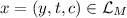
• Soundness: For every polynomial $\mathsf {T}=\mathsf {T}(\kappa )$ and for every polynomial size cheating prover $\mathsf {P}^*$ there exists a negligible function $\mu$ such that for every :

  

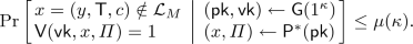
Incremental Updates. A verifiable computation scheme (with either public or designated verifier) satisfying Definition 3.2 is incrementally verifiable if given the honest proof $\varPi _t$ for a statement $(y,t,c_t)$ and the configuration $c_{t}$ we can obtain the next proof $\varPi _{t+1}$ for the statement $(y,t+1,c_{t+1})$ without repeating the entire computation. Formally, an incrementally verifiable computation scheme also includes a deterministic polynomial-time algorithm $\mathsf {Update}$ with the following syntax: given the prover key $\mathsf {pk}$, a statement $(y,t-1,c_{t-1}) \in \mathcal {L}_M$ and a proof $\varPi _{t-1}$, $\mathsf {Update}$ outputs a new proof $\varPi _{t}$. For every statement $x= (y,t,c)\in \mathcal {L}_M$, the proof $\varPi _t= \mathsf {P}(\mathsf {pk},1^t,x)$ can be constructed by running $\mathsf {Update}$ as follows:

• 1. Let $c_{0}$ be the initial configuration of $M(y)$ and let $\varPi _0 = \bot$.

• 2. For every ${\tau }\in [t]$, update $M$’s configuration from $c_{{\tau }-1}$ to $c_{\tau }$ and let:

  $$\varPi _{\tau }\leftarrow \mathsf {Update}(\mathsf {pk},\left( y,{\tau }-1,c_{{\tau }-1}\right) ,\varPi _{{\tau }-1}).$$

• 3. Output $\varPi _{t}$.

The completeness, efficiency, and soundness requirements of

4 PCP Construction

In this section we introduce notation and describe the PCP system. The update procedure for this PCP is described in the full version of this work. Before reading the full details, we recommend the reader familiarize themselves with the overview in Sect. 2.

4.1 Preliminaries

We start by introducing notations and simple clams that are used throughout the following sections.

Operations on Strings. For an alphabet $\varSigma$, a string $\mathbf {v}= v_1,\dots ,v_n \in \varSigma ^n$ and $1\le i\le j\le n$ we denote by $\mathbf {v}[i{:}j]$ the substring $v_i,\dots ,v_j$. We shorthand $\mathbf {v}[1{:}i]$ by $\mathbf {v}[{:}i]$ and $\mathbf {v}[j{:}n]$ by $\mathbf {v}[j{:}]$. We also define $\mathbf {v}[{:}0]$ and $\mathbf {v}[n+1{:}]$ to be the empty string. For a pair of strings $\mathbf {u},\mathbf {v}\in \varSigma ^n$ and $i\in [0,n]$ let $\left( \mathbf {u}|\mathbf {v}\right) _{i}$ denote the string $(\mathbf {u}[{:}i],\mathbf {v}[i+1{:}])$.

The Field $\mathbb {F}$. Fix any field $\mathbb {F}$ and a subset $\mathbb {H}\subseteq \mathbb {F}$. (The sizes of $\mathbb {F}$ and $\mathbb {H}$ will be set later in this section.) We also fix a linear order on $\mathbb {H}$ and use the lexicographical order on strings in $\mathbb {H}^m$ for any $m\in \mathbb {N}$. We denote the minimal and maximal element in $\mathbb {H}$ by $0$ and $|\mathbb {H}|-1$ respectively. For $\mathbf {t}\in \mathbb {H}^m$ such that $\mathbf {t}> 0^m$ we denote the predecessor of $\mathbf {t}$ by $\mathbf {t}-1$.

Arithmetic Circuits. We denote by $C:\mathbb {F}^i\rightarrow \mathbb {F}^j$ an arithmetic circuit over a field $\mathbb {F}$ with i input wires and j output wires. The circuit is constructed from addition, subtraction and multiplication gates of arity 2 as well as constants from $\mathbb {F}$. The size of C is the number of gates in C. We say that C is of degree d if the polynomial computed by C over $\mathbb {F}$ is of degree d or less in every one of its input variables.

Useful Predicates. We make use of arithmetic circuits computing simple predicates.

Claim 4.1

For every $i \in \mathbb {N}$ there exist arithmetic circuits $\mathsf {ID}_i,\mathsf {LE}_i,\mathsf {PR}_i:\mathbb {F}^{2i} \rightarrow \mathbb {F}$ of size O(i) and degree $|\mathbb {H}|-1$ such that for every input $\mathbf {u},\mathbf {v}\in \mathbb {H}^i$, the circuits’ output is in $\left\{ 0,1\right\}$ and:

$$\begin{aligned} \mathsf {ID}_i(\mathbf {u},\mathbf {v}) = 1&\quad \Leftrightarrow \quad \mathbf {u}= \mathbf {v}&\textit{(Identity)}\\ \mathsf {LE}_i(\mathbf {u},\mathbf {v}) = 1&\quad \Leftrightarrow \quad \mathbf {u}\le \mathbf {v}&\textit{(Lesser-or-equal)}\\ \mathsf {PR}_i(\mathbf {u},\mathbf {v}) = 1&\quad \Leftrightarrow \quad \mathbf {u}- 1 = \mathbf {v}&\textit{(Predecessor)} \end{aligned}$$

Proof

For $i=1$, circuits $\mathsf {ID}_1,\mathsf {LE}_1,\mathsf {PR}_1$ exist by straightforward interpolation. For $i>1$, $u,v\in \mathbb {F}$ and $\mathbf {u},\mathbf {v}\in \mathbb {F}^{i-1}$, let $\mathbf {u}' = (u,\mathbf {u})$ and $\mathbf {v}' = (v,\mathbf {v})$. The circuit $\mathsf {ID}_{i}$ is given by:

$$\mathsf {ID}_i(\mathbf {u}',\mathbf {v}') = \mathsf {ID}_1(u,v)\cdot \mathsf {ID}_{i-1}(\mathbf {u},\mathbf {v}).$$

The circuit $\mathsf {LE}_{i}$ is given by:

$$\mathsf {LE}_i(\mathbf {u}',\mathbf {v}') = \left[ \mathsf {ID}_1(u,v)\cdot \mathsf {LE}_{i-1}(\mathbf {u},\mathbf {v})\right] +\mathsf {LE}_1(u,v)-\mathsf {ID}_1(u,v).$$

The circuit $\mathsf {PR}_{i}$ is given by:

$$\begin{aligned} \mathsf {PR}_i(\mathbf {u}',\mathbf {v}')&= \mathsf {ID}_1(u,v)\cdot \mathsf {PR}_{i-1}(\mathbf {u},\mathbf {v})\\&+ \mathsf {PR}_1(u,v)\cdot \mathsf {ID}_{i-1}(\mathbf {u},0^{i-1})\cdot \mathsf {ID}_{i-1}(\mathbf {v},\left( |\mathbb {H}|-1\right) ^{i-1})\\ \end{aligned}$$

We also rely on the following useful property of the circuits $\mathsf {ID},\mathsf {LE},\mathsf {PR}$. Intuitively, it says that in some cases, the output of the predicate can be determine from the prefix for the input (even if the rest of the input is not in $\mathbb {H}$).

Claim 4.2

For every $i\in \mathbb {N}$, $j \in [i]$, $\mathbf {t}_1 = (\mathbf {h}_1,\mathbf {f}_1), \mathbf {t}_2 = (\mathbf {h}_2,\mathbf {f}_2)\in \mathbb {H}^{j} \times \mathbb {F}^{i-j}$ and $\mathbf {h}\in \mathbb {H}^{i}$:

• $\mathbf {h}_1\ne \mathbf {h}_2 \Rightarrow \mathsf {ID}_i(\mathbf {t}_1,\mathbf {t}_2) = 0$.

• $\mathbf {h}_1>\mathbf {h}_2 \Rightarrow \mathsf {LE}_i(\mathbf {t}_1,\mathbf {t}_2) = 0$.

• $\mathbf {h}_1<\mathbf {h}_2 \Rightarrow \mathsf {LE}_i(\mathbf {t}_1,\mathbf {t}_2) = 1$.

• $(\mathbf {h}-1)[{:}j] \ne \mathbf {h}_1 \Rightarrow \mathsf {PR}_i(\mathbf {h},\mathbf {t}_1) = 0$.

The proof of Claim 4.2 follows from the next lemma.

Lemma 4.1

Let $\varphi :\mathbb {F}^i\rightarrow \mathbb {F}$ be an arithmetic circuit of degree $(|\mathbb {H}|-1)$. For every $j \in [i]$, $\mathbf {t}\in \mathbb {H}^j$ and $b\in \left\{ 0,1\right\}$:

$$\forall \mathbf {h}\in \mathbb {H}^{i-j}:\varphi (\mathbf {t},\mathbf {h})=b\quad \Rightarrow \quad \forall \mathbf {f}\in \mathbb {F}^{i-j}:\varphi (\mathbf {t},\mathbf {f})=b.$$

4.2 The Constraints

In this section we give an algebraic representation of the constraints of a computation through the notion of a constraint circuit.

The Tableau Formula. Let $M$ be a non-deterministic Turing machine with running time $\mathsf {T}= \mathsf {T}(n)$ and space complexity $\mathsf {S}= \mathsf {S}(n)$. By the Cook-Levin theorem the computation of $M$ on some input can be described by $\mathsf {T}'\cdot \mathsf {S}'$ Boolean variables where $\mathsf {T}'= \mathsf {T}\cdot \beta$ and $\mathsf {S}'= \mathsf {S}\cdot \beta$ for some constant $\beta \in \mathbb {N}$. Intuitively, we think the variables as organized in a table with $\mathsf {T}'$ rows $\mathsf {S}'$ columns. The variables in row $\beta \cdot t$ correspond to the configuration of $M$ after $t$ steps. All other rows, whose indices are not a multiple of $\beta$, contain auxiliary variables used to verify the consistency of adjacent configurations. An assignment to the variables describes a valid computation of $M$ (with any witness) if and only if it satisfies a 3CNF “tableau formula” $\phi _y$.

Claim 4.3

(Cook-Levin-Karp.) There exists a constant $\beta$ such that for every input $y\in \left\{ 0,1\right\} ^n$ there exists a 3CNF formula $\phi _y$ over the variables $\left\{ x_{t,s}\right\} _{t\in [\mathsf {T}'], s\in [\mathsf {S}']}$ where $\mathsf {T}'= \beta \cdot \mathsf {T}$ and $\mathsf {S}'= \beta \cdot \mathsf {S}$ such that the following holds:

• Completeness: For every witness $w\in \left\{ 0,1\right\} ^\mathsf {T}$ there exists an assignment $X^{y,w}:[\mathsf {T}']\times [\mathsf {S}']\rightarrow \left\{ 0,1\right\}$ that satisfies $\phi _y$. Moreover, for any $t\in [\mathsf {T}]$, given only the configuration $c_t= M(y;w[{:}t])$ we can compute a row assignment $\gamma ^{c_t}:[\mathsf {S}']\rightarrow \left\{ 0,1\right\}$ such that $X^{y,w}(t\cdot \beta ,\cdot ) = \gamma ^{c_t}$. Similarly, for any $(t-1)\cdot \beta <{\tau }\le t\cdot \beta$, given only the configuration $c_{t-1} = M(y;w[{:}t-1])$ and the witness bit $w_t$ we can compute a row assignment $\gamma ^{c_{t-1},w_t}_{\tau }:[\mathsf {S}']\rightarrow \left\{ 0,1\right\}$ such that $X^{y,w}({\tau },\cdot ) = \gamma ^{c_{t-1},w_t}_{\tau }$.

• Soundness: For any assignment $X:[\mathsf {T}']\times [\mathsf {S}']\rightarrow \left\{ 0,1\right\}$ that satisfies $\phi _y$ there exists a witness $w$ such that $X= X^{y,w}$. Moreover, for every $t\in [\mathsf {T}]$ and configuration $c$, if $X(t\cdot \beta ,\cdot ) = \gamma ^{c}$ then $c= M(y;w[{:}t])$.

• Leveled structure: Every constraint in $\phi _y$ is of the form $\left( x_{t_1,s_1}=b_1\right) \vee \left( x_{t_2,s_2}=b_2\right) \vee \left( x_{t_3,s_3}=b_3\right)$ where $t_1 - 1 = t_2 = t_3$.

The Configuration Formula. For every ${\tau }\in [\mathsf {T}']$ and a row assignment $\gamma :[\mathsf {S}']\rightarrow \left\{ 0,1\right\}$ we define a 3CNF “configuration formula” $\phi _{{\tau },\gamma }$ over the same variables as the tableau formula $\phi _y$ checking that the ${\tau }$-th row assignment is equal to $\gamma$. That is:

• If ${\tau }= t\cdot \beta$ for some $t\in [\mathsf {T}]$ then $\phi _{{\tau },\gamma }$ is satisfied by an assignments $X:[\mathsf {T}']\times [\mathsf {S}']\rightarrow \left\{ 0,1\right\}$ if and only if $X({\tau },\cdot ) = \gamma$.

• Otherwise, $\phi _{{\tau },\gamma } = 1$ is the empty formula.

For technical reasons, we assume WLOG that all the constraints in $\phi _{{\tau },\gamma }$ are of the form $\left( x_{t_1,s_1}=b_1\right) \vee \left( x_{t_2,s_2}=b_2\right) \vee \left( x_{t_3,s_3}=b_3\right)$, where ${\tau }= t_1$. Additionally we assume that $\phi _{{\tau },\gamma }$ has the same leveled structure as the tableau formula. That is, $t_1 - 1 = t_2 = t_3$. For ${\tau }$ that is not a multiple of $\beta$, $\phi _{{\tau },\gamma }$ is the empty formula so our assumptions on the structure of $\phi _{{\tau },\gamma }$ hold vacuously.

Arithmetizing the Constraint Formula. Let $\mathbb {F}$ be a field of size $\varTheta (\log ^2{\mathsf {T}'})$, let $\mathbb {H}\subset \mathbb {F}$ be a subset of size $\lceil \log {\mathsf {T}'}\rceil$ such that $\left\{ 0,1\right\} \subseteq \mathbb {H}$ and let

$$m= \frac{\log {\mathsf {T}'}}{\log {\log {\mathsf {T}'}}}, k= \frac{\log {\mathsf {S}'}}{\log {\log {\mathsf {T}'}}}.$$

We assume WLOG that $m,k$ and $\log {\mathsf {T}'}$ are all integers and, therefore, $|\mathbb {H}^m| = \mathsf {T}'$ and $|\mathbb {H}^k| = \mathsf {S}'$. We identify elements of $\mathbb {H}^m$ (with lexicographic order) with indices in $[\mathsf {T}]$, and elements in $\mathbb {H}^k$ with indices in $[\mathsf {S}]$. We view an assignment $X$ for the variables $\left\{ x_{t,s}\right\}$ as a function $X:\mathbb {H}^{m+k} \rightarrow \left\{ 0,1\right\}$.

Constraint Circuits. We can implicitly represent a 3CNF formula $\phi$ over the variables $\left\{ x_{t,s}\right\}$ using a multivariate polynomial. Intuitively, this polynomial represents the indicator function indicating whether a given 3-disjunction is in the formula. We represent this polynomial via an arithmetic circuit over $\mathbb {F}$.

Definition 4.1

(Constraint circuit). An arithmetic circuit $\varphi :\mathbb {F}^{3(m+k+1)} \rightarrow \mathbb {F}$ is a constraint circuit representing a 3CNF formula $\phi$ over the variables $\left\{ x_{\mathbf {t},\mathbf {s}}\right\} _{\mathbf {t}\in \mathbb {H}^m, \mathbf {s}\in \mathbb {H}^k}$ if for every $\mathbf {t}_1,\mathbf {t}_2,\mathbf {t}_3\in \mathbb {H}^m$, $\mathbf {s}_1,\mathbf {s}_2,\mathbf {s}_3\in \mathbb {H}^k$ and $b_1,b_2,b_3\in \left\{ 0,1\right\}$ if $\phi$ contains the constraint:

$$\left( x_{t_1,s_1}=b_1\right) \vee \left( x_{t_2,s_2}=b_2\right) \vee \left( x_{t_3,s_3}=b_3\right) ,$$

then $\varphi$ evaluates to 1 on $(\mathbf {t}_1,\mathbf {t}_2,\mathbf {t}_3,\mathbf {s}_1,\mathbf {s}_2,\mathbf {s}_3,b_1,b_2,b_3)$. Otherwise $\varphi$ evaluates to 0.

Next, we claim that the tableau formula and configuration formula can be efficiently represented as constraint circuits.

Claim 4.4

For every input $y\in \left\{ 0,1\right\} ^n$, ${\tau }\in [\mathsf {T}']$ and assignment $\gamma :\mathbb {H}^k\rightarrow \left\{ 0,1\right\}$ let $\phi _y$ and $\phi _{{\tau },\gamma }$ be the tableau formula and the configuration formula defined above.

• Given $y$ we can efficiently compute a tableau constraint circuit $\varphi _y$ of size $O(n) + \mathrm {poly}(m)$ and degree $\mathrm {poly}(m,k)$ describing $\phi _y$.

• Given ${\tau }$ and $\gamma$ we can efficiently compute a configuration constraint circuit $\varphi _{{\tau },\gamma }$ of size $\mathsf {S}\cdot \mathrm {poly}(m)$ and degree O(1) describing $\phi _{{\tau },\gamma }$.

The Constraint Circuit ${\tilde{\varphi }}$. The constraint circuit ${\tilde{\varphi }}$ used in our PCP construction is a combination of the constraint circuit and predicates above. Let $\phi _y$ and $\phi _{{\tau },\gamma }$ be the tableau and configuration formulas defined above and let $\varphi _y$ and $\varphi _{{\tau },\gamma }$ be the constraint circuits that describe them, given by Claim 4.4. For $\mathbf {t}_1,\mathbf {t}_2,\mathbf {t}_3 \in \mathbb {F}^{m}$ and $\mathbf {f}\in \mathbb {F}^{3k+3}$, let ${\tilde{\varphi }}_{y,{\tau },\gamma }$ be the circuit give by:

$$\begin{aligned}&{\tilde{\varphi }}_{y,{\tau },\gamma }(\mathbf {t}_1,\mathbf {t}_2,\mathbf {t}_3,\mathbf {f})\\&\quad = \mathsf {PR}_{m}(\mathbf {t}_1,\mathbf {t}_2)\cdot \mathsf {PR}_{m}(\mathbf {t}_1,\mathbf {t}_3)\cdot \left( \varphi _y(\mathbf {t}_1,\mathbf {t}_2,\mathbf {t}_3,\mathbf {f}) + \mathsf {ID}_{m}({\tau },\mathbf {t}_1)\cdot \varphi _{{\tau },\gamma }(\mathbf {t}_1,\mathbf {t}_2,\mathbf {t}_3,\mathbf {f})\right) . \end{aligned}$$

Claim 4.5

For every $y\in \left\{ 0,1\right\} ^n$, ${\tau }\in \mathbb {H}^m$, $\gamma :\mathbb {H}^k\rightarrow \left\{ 0,1\right\}$, ${\tilde{\varphi }}_{y,{\tau },\gamma }$ describes the 3CNF formula $\phi _y\wedge \phi _{{\tau },\gamma }$. Moreover, for every ${\tau }' \in \mathbb {H}^m$, $\gamma ':\mathbb {H}^k\rightarrow \left\{ 0,1\right\}$, $i<m$, $\mathbf {t}_1,\mathbf {t}_2,\mathbf {t}_3\in \mathbb {H}^i\times \mathbb {F}^{m-i}$, $\mathbf {h}\in \mathbb {H}^{m}$ and $\mathbf {f}\in \mathbb {F}^{3k+3}$:

$$\begin{aligned} \left\{ \mathbf {t}_2[{:}i],\mathbf {t}_3[{:}i]\right\} \ne \left\{ (\mathbf {h}-1)[{:}i]\right\} \quad&\Rightarrow \quad {\tilde{\varphi }}_{y,{\tau },\gamma }(\mathbf {h},\mathbf {t}_2,\mathbf {t}_3 ,\mathbf {f}) = 0,\\ \mathbf {t}_1[{:}i] \notin \left\{ {\tau }[{:}i],{\tau }'[{:}i]\right\} \quad&\Rightarrow \quad {\tilde{\varphi }}_{y,{\tau },\gamma }(\mathbf {t}_1,\mathbf {t}_2,\mathbf {t}_3,\mathbf {f}) = {\tilde{\varphi }}_{y,{\tau }',\gamma '}(\mathbf {t}_1,\mathbf {t}_2,\mathbf {t}_3 ,\mathbf {f}). \end{aligned}$$

Proof

(Proof sketch). Since the tableau constraints and the configuration constraints are disjoint, the circuit $\varphi _y+ \varphi _{{\tau },\gamma }$ describes the 3CNF formula $\phi _y\wedge \phi _{{\tau },\gamma }$. By the leveled structure of the formulas $\phi _y$ and $\phi _{{\tau },\gamma }$ the circuit $\varphi _y+ \varphi _{{\tau },\gamma }$ identifies with ${\tilde{\varphi }}_{y,{\tau },\gamma }$ on $\mathbb {H}^{3(m+k+1)}$. The rest of the claim follows from the leveled structure of the formulas $\phi _y$ and $\phi _{{\tau },\gamma }$ and by Claim 4.2.

4.3 The Proof String

Recall that for every $t\in [\mathsf {T}]$ and $z\in [\ell ]$, $\sigma _{t}^z\in \varSigma$ denotes the $z$-th symbol of the proof after $t$ updates. We start by specifying the value of $\sigma _{t}^z$ and in the next section we describe the procedure $\mathsf {Update}$ maintaining it. Next we introduce some notation and describe the different components of the PCP. See Sect. 2 for a high level overview of the construction.

The first part of our construction closely follows the PCP of BFLS. Fix $y\in \left\{ 0,1\right\} ^n$ and $w\in \left\{ 0,1\right\} ^\mathsf {T}$ and let $X^{y,w}$ be the assignment given by Claim 4.3. For ${\tau }\in \mathbb {H}^m$ we define:

• Let $\gamma _{\tau }:\mathbb {H}^k\rightarrow \left\{ 0,1\right\}$ be the row assignment $\gamma _{\tau }= X^{y,w}({\tau },\cdot )$.

• Let $X_{{\tau }}:\mathbb {H}^{m+k}\rightarrow \left\{ 0,1\right\}$ be the assignment such that $X_{{\tau }}(\mathbf {t},\cdot ) = \gamma _\mathbf {t}$ for all $\mathbf {t}\le {\tau }$ and for all $\mathbf {t}> {\tau }$, $X_{{\tau }}(\mathbf {t},\cdot )$ is identically zero.

• Let ${\tilde{X}}_{{\tau }}:\mathbb {F}^{m+k}\rightarrow \mathbb {F}$ be the polynomial of degree $|\mathbb {H}|-1$ that identifies with $X_{{\tau }}$ on $\mathbb {H}^{m+k}$:

  $$\begin{aligned} {\tilde{X}}_{{\tau }}\left( \mathbf {f}\right) = \sum _{\mathbf {h}\in \mathbb {H}^{m+k}}{\mathsf {ID}\left( \mathbf {h},\mathbf {f}\right) \cdot X_{{\tau }}\left( \mathbf {h}\right) } \end{aligned}$$

• Let $Q_{{\tau }}^0:\mathbb {F}^{3(m+k+1)}\rightarrow \mathbb {F}$ be the following polynomial. For $\mathbf {z}= \left( \mathbf {t}_1,\mathbf {t}_2,\mathbf {t}_3,\mathbf {s}_1,\mathbf {s}_2,\mathbf {s}_3\right) \in \mathbb {F}^{3(m+k)}$, $\mathbf {b}= \left( b_1,b_2,b_3\right) \in \mathbb {F}^3$ and ${\bar{\mathbf {z}}}= \left( \mathbf {z},\mathbf {b}\right)$:

  $$\begin{aligned} Q_{{\tau }}^0\left( {\bar{\mathbf {z}}}\right)&= \mathsf {LE}\left( \mathbf {t}_1,{\tau }\right) \cdot {\tilde{\varphi }}_{y,{\tau },\gamma _{\tau }}\left( {\bar{\mathbf {z}}}\right) \cdot \prod _{i\in [3]}{\left( {\tilde{X}}_{{\tau }}\left( \mathbf {t}_i,\mathbf {s}_i\right) - b_i\right) }. \end{aligned}$$

• For $j \in [3(m+k)]$ let $Q_{{\tau }}^j:\mathbb {F}^{3(m+k+1)}\rightarrow \mathbb {F}$ be the polynomial:

  $$Q_{{\tau }}^j\left( \mathbf {f}\right) = \sum _{\mathbf {h}\in \mathbb {H}^j}{\mathsf {ID}\left( \mathbf {h},\mathbf {f}[{:}j]\right) \cdot Q_{{\tau }}^0\left( \mathbf {h},\mathbf {f}[j+1{:}]\right) }.$$

Next we introduce additional polynomials that are not a part of the BFLS construction). These polynomials define the supplemental values added to the PCP to support updates.

First we define polynomials $A_{{\tau }}^0,B_{{\tau }}^0,C_{{\tau }}^0$ by multiplying together subsets of the factors of $Q_{{\tau }}^0$. Let $A_{{\tau }}^0,B_{{\tau }}^0,C_{{\tau }}^0:\mathbb {F}^{3(m+k+1)}\rightarrow \mathbb {F}$ be the following polynomials. For $\mathbf {z}= \left( \mathbf {t}_1,\mathbf {t}_2,\mathbf {t}_3,\mathbf {s}_1,\mathbf {s}_2,\mathbf {s}_3\right) \in \mathbb {F}^{3(m+k)}$, $\mathbf {b}= \left( b_1,b_2,b_3\right) \in \mathbb {F}^3$, and ${\bar{\mathbf {z}}}= \left( \mathbf {z},\mathbf {b}\right)$:

$$\begin{aligned} A_{{\tau }}^0\left( {\bar{\mathbf {z}}}\right)&= {\tilde{\varphi }}_{y,{\tau },\gamma _{{\tau }}}\left( {\bar{\mathbf {z}}}\right) \cdot \left( {\tilde{X}}_{{\tau }}\left( \mathbf {t}_1,\mathbf {s}_1\right) - b_1\right) ,\\ B_{{\tau }}^0\left( {\bar{\mathbf {z}}}\right)&= {\tilde{\varphi }}_{y,{\tau },\gamma _{{\tau }}}\left( {\bar{\mathbf {z}}}\right) \cdot \left( {\tilde{X}}_{{\tau }}\left( \mathbf {t}_1,\mathbf {s}_1\right) - b_1\right) \cdot \left( {\tilde{X}}_{{\tau }}\left( \mathbf {t}_2,\mathbf {s}_2\right) - b_2\right) ,\\ C_{{\tau }}^0\left( {\bar{\mathbf {z}}}\right)&= {\tilde{\varphi }}_{y,{\tau },\gamma _{{\tau }}}\left( {\bar{\mathbf {z}}}\right) \cdot \left( {\tilde{X}}_{{\tau }}\left( \mathbf {t}_1,\mathbf {s}_1\right) - b_1\right) \cdot \left( {\tilde{X}}_{{\tau }}\left( \mathbf {t}_2,\mathbf {s}_2\right) - b_2\right) \cdot \left( {\tilde{X}}_{{\tau }}\left( \mathbf {t}_3,\mathbf {s}_3\right) - b_3\right) . \end{aligned}$$

Next we define the polynomials $A_{{\tau }}^j,B_{{\tau }}^j,C_{{\tau }}^j$. Similar to the definition of $Q_{{\tau }}^j$ via $Q_{{\tau }}^0$, the evaluations of $A_{{\tau }}^j,B_{{\tau }}^j$ and $C_{{\tau }}^j$ on input ${\bar{\mathbf {z}}}\in \mathbb {F}^{3(m+k+1)}$ are given by a weighted sum of evaluations of $A_{{\tau }}^0,B_{{\tau }}^0$ and $C_{{\tau }}^0$ respectively, over inputs ${\bar{\mathbf {z}}}'$ whose prefix is in $\mathbb {H}$ and suffix in equal to that of ${\bar{\mathbf {z}}}$. However, unlike the definition of $Q_{{\tau }}^j$, we do not sum over all possible prefixes in $\mathbb {H}$, but only over prefixes with a certain structure. Specifically:

• $A_{{\tau }}^j$ sums over prefixes $\mathbf {h}\in \mathbb {H}^j$ such that $\mathbf {h}< {\tau }[{:}j]$.

• $B_{{\tau }}^j$ sums over prefixes $(\mathbf {h}, (\mathbf {h}-1)[{:}j])\in \mathbb {H}^{m+j}$ such that $0^m< \mathbf {h}< {\tau }$.

• $C_{{\tau }}^j$ sums over prefixes $(\mathbf {h}, \mathbf {h}-1,(\mathbf {h}-1)[{:}j])\in \mathbb {H}^{2m+j}$ such that $0^m< \mathbf {h}< {\tau }$.

Formally, for $j \in [m]$ let $A_{{\tau }}^j,B_{{\tau }}^j,C_{{\tau }}^j:\mathbb {F}^{3(m+k+1)}\rightarrow \mathbb {F}$ be the following polynomials. For $\mathbf {z}= \left( \mathbf {t}_1,\mathbf {t}_2,\mathbf {t}_3,\mathbf {s}_1,\mathbf {s}_2,\mathbf {s}_3\right) \in \mathbb {F}^{3(m+k)}$, $\mathbf {b}= \left( b_1,b_2,b_3\right) \in \mathbb {F}^3$ and ${\bar{\mathbf {z}}}= \left( \mathbf {z},\mathbf {b}\right)$:

$$\begin{aligned} A_{{\tau }}^j({\bar{\mathbf {z}}})&= \sum _{\mathbf {h}< {\tau }[{:}j]}{\mathsf {ID}\left( \mathbf {h},{\bar{\mathbf {z}}}[{:}j]\right) \cdot A_{{\tau }}^0\left( \mathbf {h},{\bar{\mathbf {z}}}[j+1{:}]\right) },\\ B_{{\tau }}^j({\bar{\mathbf {z}}})&= \sum _{0^m< \mathbf {h}< {\tau }}{\mathsf {ID}\left( \left( \mathbf {h},(\mathbf {h}-1)[{:}j]\right) ,{\bar{\mathbf {z}}}[{:}m+j]\right) \cdot B_{{\tau }}^0\left( \left( \left( \mathbf {h},\mathbf {h}-1\right) |{\bar{\mathbf {z}}}\right) _{m+j}\right) },\\ C_{{\tau }}^j({\bar{\mathbf {z}}})&= \sum _{0^m< \mathbf {h}< {\tau }}\mathsf {ID}\left( \left( \mathbf {h},\mathbf {h}-1,(\mathbf {h}-1)[{:}j]\right) ,{\bar{\mathbf {z}}}[{:}2m+j]\right) \cdot C_{{\tau }}^0\left( \left( \left( \mathbf {h},\mathbf {h}-1,\mathbf {h}-1\right) |{\bar{\mathbf {z}}}\right) _{2m+j}\right) . \end{aligned}$$

Finally, we define polynomials ${\bar{A}}_{{\tau }}^j,{\bar{B}}_{{\tau }}^j,{\bar{C}}_{{\tau }}^j$. These are defined similarly to $A_{{\tau }}^j,B_{{\tau }}^j,C_{{\tau }}^j$ except that we sum over different prefixes:

• ${\bar{A}}_{{\tau }}^j$ sums over prefixes $(\mathbf {h}, (\mathbf {h}-1)[{:}j])\in \mathbb {H}^{m+j}$ such that $0^m< \mathbf {h}< {\tau }$ and $(\mathbf {h}-1)[{:}j] = {\tau }[{:}j]$.

• ${\bar{B}}_{{\tau }}^j$ sums over prefixes $(\mathbf {h}, \mathbf {h}-1,(\mathbf {h}-1)[{:}j])\in \mathbb {H}^{2m+j}$ such that $0^m< \mathbf {h}< {\tau }$ and $(\mathbf {h}-1)[{:}j] = {\tau }[{:}j]$.

• ${\bar{C}}_{{\tau }}^j$ sums over prefixes $(\mathbf {h}, \mathbf {h}-1,\mathbf {h}-1,\mathbf {h}')\in \mathbb {H}^{3m+j}$ such that $0^m< \mathbf {h}< {\tau }$ and $\mathbf {h}' \in \mathbb {H}^j$.

Formally, for $j \in [m]$ let ${\bar{A}}_{{\tau }}^j,{\bar{B}}_{{\tau }}^j:\mathbb {F}^{3(m+k+1)}\rightarrow \mathbb {F}$ be the following polynomials. For $\mathbf {z}= \left( \mathbf {t}_1,\mathbf {t}_2,\mathbf {t}_3,\mathbf {s}_1,\mathbf {s}_2,\mathbf {s}_3\right) \in \mathbb {F}^{3(m+k)}$, $\mathbf {b}= \left( b_1,b_2,b_3\right) \in \mathbb {F}^3$ and ${\bar{\mathbf {z}}}= \left( \mathbf {z},\mathbf {b}\right)$:

$$\begin{aligned} {\bar{A}}_{{\tau }}^j({\bar{\mathbf {z}}})&= \sum _{\begin{array}{c} 0^m< \mathbf {h}< {\tau }\\ (\mathbf {h}-1)[{:}j] = {\tau }[{:}j] \end{array}} {\mathsf {ID}\left( \left( \mathbf {h},{\tau }[{:}j]\right) ,{\bar{\mathbf {z}}}[{:}m+j]\right) \cdot A_{{\tau }}^0\left( \left( \left( \mathbf {h},{\tau }\right) |{\bar{\mathbf {z}}}\right) _{m+j}\right) },\\ {\bar{B}}_{{\tau }}^j({\bar{\mathbf {z}}})&= \sum _{\begin{array}{c} 0^m< \mathbf {h}< {\tau }\\ (\mathbf {h}-1)[{:}j] = {\tau }[{:}j] \end{array}} \mathsf {ID}\left( \left( \mathbf {h},\mathbf {h}-1,{\tau }[{:}j]\right) ,{\bar{\mathbf {z}}}[{:}2m+j]\right) \\&\quad \cdot B_{{\tau }}^0\left( \left( \left( \mathbf {h},\mathbf {h}-1,{\tau }\right) |{\bar{\mathbf {z}}}\right) _{2m+j}\right) , \end{aligned}$$

For $j \in [3k]$ let ${\bar{C}}_{{\tau }}^j:\mathbb {F}^{3(m+k+1)}\rightarrow \mathbb {F}$ be the following polynomial:

$$\begin{aligned} {\bar{C}}_{{\tau }}^j({\bar{\mathbf {z}}})&= \sum _{\begin{array}{c} 0^m< \mathbf {h}< {\tau }\\ \mathbf {h}' \in \mathbb {H}^j \end{array}}\mathsf {ID}\left( \left( \mathbf {h},\mathbf {h}-1,\mathbf {h}-1,\mathbf {h}'\right) ,{\bar{\mathbf {z}}}[{:}3m+j]\right) \\&\quad \cdot C_{{\tau }}^0\left( \mathbf {h},\mathbf {h}-1,\mathbf {h}-1,\mathbf {h}',{\bar{\mathbf {z}}}[3m+j+1{:}]\right) . \end{aligned}$$

We are now ready to define the PCP proof string. We set $\ell = |\mathbb {F}|^{3(m+k)}$ and identify elements of $\mathbb {F}^{3(m+k)}$ with indices in $[\ell ]$.

We first define for every ${\tau }\in \mathbb {H}^m$ and $\mathbf {z}= (\mathbf {t}_1,\mathbf {t}_2,\mathbf {t}_3,\mathbf {s}_1,\mathbf {s}_2,\mathbf {s}_3) \in \mathbb {F}^{3(m+k)}$ an auxiliary symbol ${\bar{\sigma }}_{{\tau }}^\mathbf {z}$. These auxiliary symbols will be useful in defining the update procedure. Then, for every $t\in [\mathsf {T}]$, we set the proof symbol $\sigma _{t}^\mathbf {z}$ to be the symbol ${\bar{\sigma }}_{t\cdot \beta }^\mathbf {z}$. The auxiliary symbol ${\bar{\sigma }}_{{\tau }}^\mathbf {z}$ contains the values:

• 1. ${\tilde{X}}_{{\tau }}(\left( {\tau }|\mathbf {t}_i\right) _{j},\mathbf {s}_i)$ for every $i \in [3]$ and $j \in [0,m]$.

• 2. ${\tilde{X}}_{{\tau }}(\left( {\tau }-1|\mathbf {t}_i\right) _{j},\mathbf {s}_i)$ for every $i \in [3]$ and $j \in [0,m]$. (Only if ${\tau }> 0^m$.)

• 3. $Q_{{\tau }}^j(\mathbf {z},\mathbf {b})$ for every $j \in [0,3(m+k)]$ and $\mathbf {b}\in \left\{ 0,1\right\} ^3$.

• 4. $A_{{\tau }}^j(\mathbf {z},\mathbf {b}), {\bar{A}}_{{\tau }}^j(\mathbf {z},\mathbf {b}), B_{{\tau }}^j(\mathbf {z},\mathbf {b}), {\bar{B}}_{{\tau }}^j(\mathbf {z},\mathbf {b}), C_{{\tau }}^j(\mathbf {z},\mathbf {b})$ for every $j \in [m]$ and $\mathbf {b}\in \left\{ 0,1\right\} ^3$.

• 5. ${\bar{C}}_{{\tau }}^j(\mathbf {z},\mathbf {b})$ for every $j \in [3k]$ and $\mathbf {b}\in \left\{ 0,1\right\} ^3$.

The following theorem (that follows from the proof of [BFLS91]) states that the construction above is indeed a PCP proof. In the following sections we prove that this PCP is incrementally updatable.

Theorem 4.6

(Follows from [BFLS91]). There exists a PCP system $(\mathsf {P},\mathsf {V})$ for $M$ with alphabet $\varSigma = \mathbb {F}^{O(m+ k)}$, query complexity $q= \mathrm {poly}(m+ k)$, and proof length $\ell = |\mathbb {F}|^{3(m+k)} = \mathrm {poly}(\mathsf {T}\cdot \mathsf {S})$ such that given $((y,t,c),w)\in \mathcal {R}_M$, $\mathsf {P}$ outputs the proof $\varPi = \left( \sigma _{t}^1,\dots ,\sigma _{t}^{\ell }\right)$.

References

Bitansky, N., et al.: The hunting of the SNARK. J. Cryptol. 30(4), 989–1066 (2017)
Bitansky, N., Canetti, R., Chiesa, A., Tromer, E.: Recursive composition and bootstrapping for snarks and proof-carrying data. In: STOC, pp. 111–120 (2013)
Babai, L., Fortnow, L., Levin, L.A., Szegedy, M.: Checking computations in polylogarithmic time. In: Proceedings of the 23rd Annual ACM Symposium on Theory of Computing, New Orleans, Louisiana, USA, 5–8 May 1991, pp. 21–31 (1991)
Brakerski, Z., Holmgren, J., Kalai, Y.T.: Non-interactive RAM and batch NP delegation from any PIR. IACR Cryptology ePrint Archive, 2016:459 (2016)
Brakerski, Z., Holmgren, J., Kalai, Y.T.: Non-interactive delegation and batch NP verification from standard computational assumptions. In: Proceedings of the 49th Annual ACM SIGACT Symposium on Theory of Computing, STOC 2017, Montreal, QC, Canada, 19–23 June 2017, pp. 474–482 (2017)
Biehl, I., Meyer, B., Wetzel, S.: Ensuring the integrity of agent-based computations by short proofs. In: Rothermel, K., Hohl, F. (eds.) MA 1998. LNCS, vol. 1477, pp. 183–194. Springer, Heidelberg (1998). https://doi.org/10.1007/BFb0057658
Brakerski, Z., Vaikuntanathan, V.: Efficient fully homomorphic encryption from (standard) LWE. In IEEE 52nd Annual Symposium on Foundations of Computer Science, FOCS 2011, Palm Springs, CA, USA, October 22–25, 2011, pp. 97–106 (2011)
Dodis, Y., Halevi, S., Rothblum, R.D., Wichs, D.: Spooky encryption and its applications. In: Robshaw, M., Katz, J. (eds.) CRYPTO 2016. LNCS, vol. 9816, pp. 93–122. Springer, Heidelberg (2016). https://doi.org/10.1007/978-3-662-53015-3_4
Dwork, C., Langberg, M., Naor, M., Nissim, K., Reingold, O.: Succinct proofs for \(\sf NP\) ander spooky interactions. Manuscript (2000). http://www.wisdom.weizmann.ac.il/~naor/PAPERS/spooky.pdf
Dwork, C., Naor, M., Rothblum, G.N.: Spooky interaction and its discontents: compilers for succinct two-message argument systems. In: Robshaw, M., Katz, J. (eds.) CRYPTO 2016. LNCS, vol. 9816, pp. 123–145. Springer, Heidelberg (2016). https://doi.org/10.1007/978-3-662-53015-3_5
Gentry, C.: Fully homomorphic encryption using ideal lattices. In: Proceedings of the 41st Annual ACM Symposium on Theory of Computing, STOC 2009, Bethesda, MD, USA, 31 May–2 June, pp. 169–178 (2009)
Goldreich, O., Håstad, J.: On the complexity of interactive proofs with bounded communication. Inf. Process. Lett. 67(4), 205–214 (1998)
Gentry, C., Sahai, A., Waters, B.: Homomorphic encryption from learning with errors: conceptually-simpler, asymptotically-faster, attribute-based. In: Canetti, R., Garay, J.A. (eds.) CRYPTO 2013. LNCS, vol. 8042, pp. 75–92. Springer, Heidelberg (2013). https://doi.org/10.1007/978-3-642-40041-4_5
Holmgren, J., Rothblum, R.: Delegating computations with (almost) minimal time and space overhead. In: 59th IEEE Annual Symposium on Foundations of Computer Science, FOCS 2018, Paris, France, 7–9 October 2018, pp. 124–135 (2018)
Kalai, Y., Paneth, O., Yang, L.: How to delegate computations publicly. In: STOC (2019)
Kalai, Y.T., Raz, R., Rothblum, R.D.: Delegation for bounded space. In: STOC, pp. 565–574 (2013)
Kalai, Y.T., Raz, R., Rothblum, R.D.: How to delegate computations: the power of no-signaling proofs. In: Symposium on Theory of Computing, STOC 2014, New York, NY, USA, 31 May–03 June 2014, pp. 485–494 (2014)
Paneth, O., Rothblum, G.N.: On zero-testable homomorphic encryption and publicly verifiable non-interactive arguments. In: Kalai, Y., Reyzin, L. (eds.) TCC 2017. LNCS, vol. 10678, pp. 283–315. Springer, Cham (2017). https://doi.org/10.1007/978-3-319-70503-3_9
Valiant, P.: Incrementally verifiable computation or proofs of knowledge imply time/space efficiency. In: Canetti, R. (ed.) TCC 2008. LNCS, vol. 4948, pp. 1–18. Springer, Heidelberg (2008). https://doi.org/10.1007/978-3-540-78524-8_1
Author information
Authors and Affiliations
Corresponding author
Editor information
Editors and Affiliations
Rights and permissions
Copyright information
© 2019 International Association for Cryptologic Research
About this paper
Cite this paper
Naor, M., Paneth, O., Rothblum, G.N. (2019). Incrementally Verifiable Computation via Incremental PCPs. In: Hofheinz, D., Rosen, A. (eds) Theory of Cryptography. TCC 2019. Lecture Notes in Computer Science(), vol 11892. Springer, Cham. https://doi.org/10.1007/978-3-030-36033-7_21
Download citation
DOI: https://doi.org/10.1007/978-3-030-36033-7_21
Published:
Publisher Name: Springer, Cham
Print ISBN: 978-3-030-36032-0
Online ISBN: 978-3-030-36033-7
eBook Packages: Computer ScienceComputer Science (R0)