
Abstract
We present a new general framework for constructing compact and adaptively secure attribute-based encryption (ABE) schemes from k-Lin in asymmetric bilinear pairing groups. Previously, the only construction [Kowalczyk and Wee, Eurocrypt ’19] that simultaneously achieves compactness and adaptive security from static assumptions supports policies represented by Boolean formulae. Our framework enables supporting more expressive policies represented by arithmetic branching programs.
Our framework extends to ABE for policies represented by uniform models of computation such as Turing machines. Such policies enjoy the feature of being applicable to attributes of arbitrary lengths. We obtain the first compact adaptively secure ABE for deterministic and non-deterministic finite automata (DFA and NFA) from k-Lin, previously unknown from any static assumptions. Beyond finite automata, we obtain the first ABE for large classes of uniform computation, captured by deterministic and non-deterministic logspace Turing machines (the complexity classes \(\mathsf {L}\) and \(\mathsf {NL}\)) based on k-Lin. Our ABE scheme has compact secret keys of size linear in the description size of the Turing machine M. The ciphertext size grows linearly in the input length, but also linearly in the time complexity, and exponentially in the space complexity. Irrespective of compactness, we stress that our scheme is the first that supports large classes of Turing machines based solely on standard assumptions. In comparison, previous ABE for general Turing machines all rely on strong primitives related to indistinguishability obfuscation.
You have full access to this open access chapter, Download conference paper PDF
1 Introduction
Attribute-based encryption (ABE) [32] is an advanced form of public-key encryption that enables fine-grained access control. The encryption algorithm using the master public key \(\mathsf {mpk}\) can encrypt a message m with a descriptive attribute x,Footnote 1 producing a ciphertext \(\mathsf {ct}_x(m)\). The key generation algorithm using the master secret key \(\mathsf {msk}\) can produce a secret key \(\mathsf {sk}_y\) associated with an access policy y. Decrypting \(\mathsf {ct}_x(m)\) using \(\mathsf {sk}_y\) reveals the message m if the attribute x satisfies the policy y; otherwise, no information about m is revealed. The security requirement of ABE stipulates resilience to collusion attacks—any group of users holding secret keys for different policies learn nothing about the plaintext as long as none of them is individually authorized to decrypt the ciphertext.
A primary goal of research on ABE is designing ABE schemes for expressive classes of policies, usually defined by computation models or complexity classes. A beautiful and fruitful line of works have constructed ABE for many different policy classes. For non-uniform computation, we have ABE for Boolean [32, 44] or arithmetic formulae, branching/span programs [13, 23, 31, 37, 45, 47, 48, 53, 54], and circuits [14, 19, 30]. For uniform computation, we have ABE for deterministic finite automata [1, 5, 12, 13, 29, 58], non-deterministic finite automata [4], and even Turing machines [3, 8]. These constructions, however, achieve different trade-offs between security, efficiency, and underlying computational assumptions. It is rare to have a construction that simultaneously achieves the following natural desirata on all fronts:
-
Security: (full) adaptive security (as opposed to selective or semi-adaptive security);
-
Efficiency: having compact secret key and ciphertext, whose sizes grow linearly with the description size of the policy and the length of the attribute, respectively;
-
Assumptions: relying on standard and simple assumptions, such as LWE and k-Lin or SXDH in bilinear pairing groups (in particular, it is preferable to avoid the use of strong primitives such as indistinguishability obfuscation, and instance-dependent assumptions such as q-type assumptions, whose strength can be weakened by adversarially chosen parameters).
All previous constructions of ABE fail to achieve at least one of the desirable properties, except for the recent construction of ABE for Boolean formulae from the k-Lin assumption by Kowalczyk and Wee [44]. This raises the question:
Can we construct ABE schemes with all the desirable properties above
for more expressive classes of policies than Boolean formulae?
When it comes to uniform computation, the state of affairs is even less satisfactory. All constructions of ABE for general Turing machines are based on strong primitives such as indistinguishability obfuscation and multilinear map. Without these powerful tools, existing schemes can only handle the weak computation model of finite automata.
Can we construct ABE schemes based on standard assumptions
for more expressive uniform computations than finite automata?
Our Result. Via a unified framework, we construct compact and adaptively secure ABE schemes based on the k-Lin assumption in asymmetric prime-order bilinear pairing groups for the following classes of policies:
Arithmetic Branching Programs. ABPs capture many functions of interest, including arithmetic computations like sparse polynomials, mean, and variance, as well as combinatorial computations like string-matching, finite automata, and decision trees. It is also known that Boolean/arithmetic formulae and Boolean branching programs can all be converted into ABPs with polynomial blow-up in description size. Thus, ABPs can be viewed as a more powerful computational model than them.
Previous ABE schemes for ABPs only provide selective security [30, 37] or do not have compact ciphertexts [23].Footnote 2 In addition to achieving both adaptive security and compactness, our scheme is the first one that handles ABPs directly without converting it to circuits or arithmetic span programs, which leads to an efficiency improvement in the size of the secret keys from up to quadratic to linear in the size of the ABP.Footnote 3
 Here, a secret key is associated with a Turing machine M, and the attribute in a ciphertext specifies an input \(\mathbf{x}\), a polynomial time bound T, and a logarithmic space bound S. Decryption succeeds if and only if M accepts \(\mathbf{x}\) within time T and space S. Our scheme is unbounded in the sense that the public parameters do not restrict the sizes of the Turing machine M and input \(\mathbf{x}\), nor the time/space bounds T, S. Furthermore, it enjoys the advantage of ABE for uniform computation that a secret key for M can decrypt ciphertexts with arbitrarily long inputs and arbitrary time/space bounds. This stands in contrast with ABE for non-uniform computation (like ABPs), where a program or circuit f takes inputs of a specific length n, and a secret key for f decrypts only ciphertext of length-n inputs. Achieving this feature is precisely the challenge in constructing ABE for uniform models of computation.
Our scheme is the first ABE for large classes of Turing machine computation, captured by the complexity classes \(\mathsf {L}\) and \(\mathsf {NL}\), without using the heavy machineries of multilinear map, extractable witness encryption, or indistinguishability obfuscation as in previous works [3, 9, 27, 41]. In addition, our scheme is adaptively secure and half-compact. The secret keys are compact, of size O(|M|) linear in the description size of M, while the ciphertext size depends linearly in \(|\mathbf{x}|TS2^S\) (both ignoring fixed polynomial factors in the security parameter).
Removing the dependency on \(2^S\) or T is an interesting open problem that requires technical breakthrough. In particular, removing the dependency on \(2^S\) would give an ABE for polynomial-time Turing machine computation from pairing, a long sought-after goal that has remained elusive for more than a decade. Removing the dependency of encryption time on T even only in the 1-key 1-ciphertext setting implies a succinct message-hiding encoding [42],Footnote 4 which is only known from strong primitives like indistinguishability obfuscation or functional encryption [18, 21, 41, 42]. Removing the dependency of ciphertext size on T might be an easier task, but would need new techniques different from ours.
 As a special case of ABE for \(\mathsf {L}\) and \(\mathsf {NL}\), we obtain ABE for deterministic finite automata (DFA) and non-deterministic finite automata (NFA).Footnote 5 This simply follows from the fact that DFA and NFA can be represented as simple deterministic and non-deterministic Turing machines with space complexity 1 and time complexity N that always move the input tape pointer to the right and never use the work tape.
Previous schemes for DFA based on pairing either achieve only selective security [5, 29, 58] or rely on q-type assumptions [1, 12, 13]. The only direct construction of ABE for NFA [4] based on LWE, however, is symmetric-key and only selectively secure. We settle the open problem of constructing adaptively secure ABE for DFA from static assumptions [29] and that of constructing ABE for NFA that is public-key, adaptively secure, or based on assumptions other than LWE [4].
New Techniques for Constructing Adaptively Secure ABE. Constructing adaptively secure ABE is a challenging task. Roughly speaking, previous constructions proceed in two steps. First, a secure core secret-key ABE component for a single ciphertext and a single secret key—termed 1-ABE—is designed. Then, Dual System Encryption framework, originally proposed in [57] and refined in [1, 12, 13, 22, 59], provides guidance on how to lift 1-ABE to the public-key and multi-secret-key setting. The main technical challenge lies in the first step: Adaptively secure schemes prior to that of Kowalczyk and Wee [44] either impose a read-once restriction on the attributeFootnote 6 [45, 59] or rely on q-type assumptions [1, 12, 16, 48]. Kowalczyk and Wee [44] elegantly applied the “partial selectivization” framework [6, 38] for achieving adaptive security in general to constructing 1-ABE. In particular, they used a variant of the secret-sharing scheme for Boolean formulae in [38] whose selective simulation security can be proven via a sequence of hybrids, each only requiring partial information of the input to be chosen selectively. Then, to show adaptive security, the reduction can guess this partial information while incurring only a polynomial security loss.
However, secret-sharing schemes as needed in [44] are only known for Boolean formulae. When dealing with computation over arithmetic domains of potentially exponential size, we have the additional challenge that it is hard to guess even a single component of the input, except with exponentially small probability, rendering the partial selectivization framework ineffective. When dealing with uniform computation, we further encounter the challenge that neither the secret key nor the ciphertext is as large as the secret-sharing, making it impossible to directly use information-theoretically secure secret-sharing schemes. We develop new techniques to overcome these challenges.
-
1.
First, we present a generic framework for constructing adaptively secure 1-ABE from (i) an information theoretic primitive called arithmetic key garbling, and (ii) a computational primitive called function-hiding inner-product functional encryption (IPFE) [17, 40, 49, 56]. Our arithmetic key garbling schemes are partial garbling schemes [37] with special structures, which act as the counterpart of secret-sharing schemes for arithmetic computation. Our framework is modular: It decomposes the task of constructing 1-ABE to first designing an arithmetic key garbling scheme for the computation class of interest, and second applying a generic transformation depending solely on structural properties of the garbling and agnostic of the underlying computation. In particular, the security proof of the transformation does not attempt to trace the computation, unlike [29, 44].
-
2.
Second, we formulate structural properties of arithmetic key garbling schemes—called piecewise security—sufficient for achieving adaptive security. The properties are natural and satisfied by the garbling scheme for ABPs in [37]. For logspace Turing machine computation, we present a simple arithmetic key garbling scheme for \(\mathsf {L}\) and \(\mathsf {NL}\), inspired by the garbling schemes in [11, 19].
-
3.
Third, we present a new method of lifting 1-ABE to full-fledged ABE using function-hiding IPFE. Our method can be cast into the dual system encryption framework, but is natural on its own, without seeing through the lens of dual system encryption. One feature of IPFE is that it provides a conceptually simple abstraction which allows moving information between ABE keys and ciphertexts easily, and hides away lower-level details on how to guarantee security. This feature makes it a convenient tool in many other parts of the security proof as well.
-
4.
Lastly, to overcome the unique challenge related to ABE for uniform computation, we further enhance our generic method to be able to use partial garbling generated with pseudorandomness so that the total size of the secret keys and ciphertexts can be smaller than the garbling.
Organization. In Sect. 2, we give an overview of our framework for constructing compact adaptively secure ABE schemes for ABPs, logspace Turing machines, and finite automata, using as tools IPFE and arithmetic key garbling schemes (AKGS, a refinement of partial garbling schemes). After introducing basic notations and definitions in Sect. 3, we define AKGS and its security in Sect. 4. In Sect. 5, we show how to construct 1-ABE (the core component of our ABE schemes) for ABPs from an AKGS. Due to space constraints, the security proof of our 1-ABE for ABPs, the construction of full-fledged ABE for ABPs, and ABE for \(\mathsf {L}\) and \(\mathsf {NL}\) are provided in the full version.
2 Technical Overview
We now give an overview of our technique, starting with introducing the two key tools arithmetic key garbling schemes and IPFE. Below, by bilinear pairing groups, we mean asymmetric prime-order bilinear pairing groups, denoted as \((G_1, G_2, G_\text {T}, g_1, g_2, e)\) and implicitly, \(g_\text {T}=e({g_1,g_2})\). We use \( \mathopen [\!\mathopen [{a}\mathclose ]\!\mathclose ] _b\) to represent the encoding \(g_b^a\) of a in group \(G_b\).
Arithmetic Key Garbling Scheme. We use a refinement of the notion of partial garbling schemes [37] (which in turn is based on the notion of garbling and randomized encoding [10, 36, 61]). An arithmetic key garbling scheme (AKGS) is an information-theoretic partial garbling scheme for computing \(\alpha f(\mathbf {x})+\beta \) that hides the secrets \(\alpha , \beta \in \mathbb {Z}_p\), but not \(f, \mathbf{x}\):
-
A garbling procedure \((\mathbf {L}_1,\dots ,\mathbf {L}_m) \leftarrow \mathsf {Garble}(f,\alpha ,\beta ; \mathbf{r})\) turns f and two secrets \(\alpha , \beta \) (using randomness \(\mathbf{r}\)) into m affine label functions \(L_1,\dots ,L_m\), described by their coefficient vectors \(\mathbf{L}_1, \dots , \mathbf{L}_m\) over \(\mathbb {Z}_p\). The label functions specify how to encode an input \(\mathbf{x}\) to produce the labels for computing \(f(\mathbf {x})\) with secrets \(\alpha ,\beta \):
$$\begin{aligned} \widehat{f(\mathbf{x})}_{\alpha ,\beta } = (\ell _1, \dots , \ell _m) \text {, where } \ell _j = L_j(\mathbf{x}) = \langle \mathbf{L}_j, ({1, \mathbf{x}}) \rangle \text { over }\mathbb {Z}_p. \end{aligned}$$(1) -
A linear evaluation procedure \(\gamma \leftarrow \mathsf {Eval}({f,\mathbf {x},\ell _1,\dots ,\ell _m})\) recovers the sum \(\gamma =\alpha f(\mathbf{x}) + \beta \) weighted by the function value \(f(\mathbf{x})\).
AKGS is a partial garbling as it only hides information of the secrets \(\alpha \) and \(\beta \) beyond the weighted sum \(\alpha f(\mathbf{x}) + \beta \), and does not hide \((f, \mathbf{x})\), captured by a simulation procedure  that produces the same distribution as the honest labels.
Ishai and Wee [37] proposed a partial garbling scheme for ABPs, which directly implies an AKGS for ABPs. It is also easy to observe that the (fully secure) garbling scheme for arithmetic formulae in [11] can be weakened [19] to an AKGS. Later, we will introduce additional structural and security properties of AKGS needed for our 1-ABE construction. These properties are natural and satisfied by both schemes [11, 37].
Inner-Product Functional Encryption. A function-hiding (secret-key) inner-product functional encryption (IPFE)Footnote 7 enables generating many secret keys \(\mathsf {isk}(\mathbf{v}_j)\) and ciphertexts \(\mathsf {ict}(\mathbf{u}_i)\) associated with vectors \(\mathbf{v}_j\) and \(\mathbf{u}_i\) such that decryption yields all the inner products \(\{\langle \mathbf{u}_i, \mathbf{v}_j \rangle \}_{i,j}\) (mod p) and nothing else. In this work, we need an adaptively secure IPFE, whose security holds even against adversaries choosing all the vectors adaptively. Such an IPFE scheme can be constructed based on the k-Lin assumption in bilinear pairing groups [50, 60]. The known scheme also has nice structural properties that will be instrumental to our construction of ABE:
-
 operates linearly on \(\mathbf {v}\) (in the exponent of \(G_2\)) and the size of the secret key \(\mathsf {isk}(\mathbf {v})\) grows linearly with \(|\mathbf{v}|\).
 -
 also operates linearly on \(\mathbf {u}\) (in the exponent of \(G_1\)) and the size of the ciphertext \(\mathsf {ict}(\mathbf{u})\) grows linearly with \(|\mathbf{u}|\).
 -
\(\mathsf {IPFE}.\mathsf {Dec}(\mathsf {sk}(\mathbf {v}),\mathsf {ct}(\mathbf {u}))\) simply invokes pairing to compute the inner product \( \mathopen [\!\mathopen [{\langle \mathbf {u},\mathbf {v}\rangle }\mathclose ]\!\mathclose ] _\text {T}\) in the exponent of the target group.
 operates linearly on
  also operates linearly on
 2.1 1-ABE from Arithmetic Key Garbling and IPFE Schemes
1-ABE is the technical heart of our ABE construction. It works in the setting where a single ciphertext \(\mathsf {ct}(\mathbf{x})\) for an input vector \(\mathbf {x}\) and a single secret key \(\mathsf {sk}(f, \mu )\) for a policy \(y = f_{\ne 0}\) and a secret \(\mu \) are published. Decryption reveals \(\mu \) if \(f(\mathbf{x}) \ne 0\); otherwise, \(\mu \) is hidden.Footnote 8
1-ABE. To hide \(\mu \) conditioned on \(f(\mathbf{x}) = 0\), our key idea is using IPFE to compute an AKGS garbling \(\widehat{f(\mathbf{x})}_{\mu , 0}\) of \(f(\mathbf{x})\) with secrets \(\alpha =\mu \) and \(\beta =0\). The security of AKGS guarantees that only \(\mu f(\mathbf{x})\) is revealed, which information theoretically hides \(\mu \) when \(f(\mathbf{x}) = 0\).
The reason that it is possible to use IPFE to compute the garbling is attributed to the affine input-encoding property of AKGS—the labels \(\ell _1, \dots , \ell _m\) are the output of affine functions \(L_1,\dots , L_j\) of \(\mathbf{x}\) as described in Eq. (1). Since \(f,\alpha ,\beta \) are known at key generation time, the ABE key can be a collection of IPFE secret keys, each encoding the coefficient vector \(\mathbf{L}_j\) of one label function \(L_j\). On the other hand, the ABE ciphertext can be an IPFE ciphertext encrypting \(({1,\mathbf{x}})\). When put together for decryption, they reveal exactly the labels \(L_1(\mathbf{x}), \dots , L_m(\mathbf{x})\), as described below on the left.

We note that the positions or slots at the right end of the vectors encoded in \(\mathsf {isk}\) and \(\mathsf {ict}\) are set to zero by the honest algorithms—\(\mathbf 0\) denotes a vector (of unspecified length) of zeros. These slots provide programming space in the security proof.
It is extremely simple to prove selective (or semi-adaptive) security, where the input \(\mathbf{x}\) is chosen before seeing the \(\mathsf {sk}\). By the function-hiding property of IPFE, it is indistinguishable to switch the secret keys and the ciphertext to encode any vectors that preserve the inner products. This allows us to hardwire honestly generated labels \(\widehat{f(\mathbf{x})}_{\mu ,0} = \{\ell _j \leftarrow \langle \mathbf{L}_j, ({1,\mathbf{x}})\rangle \}_{j\in [m]}\) in the secret keys as described above on the right. The simulation security of AKGS then implies that only \(\mu f(\mathbf{x})\) is revealed, i.e., nothing about \(\mu \) is revealed.
Achieving Adaptive Security. When it comes to adaptive security, where the input \(\mathbf{x}\) is chosen after seeing \(\mathsf {sk}\), we can no longer hardwire the honest labels \(\widehat{f(\mathbf{x})}_{\mu ,0}\) in the secret key, as \(\mathbf{x}\) is undefined when \(\mathsf {sk}\) is generated, and hence cannot invoke the simulation security of AKGS. Our second key idea is relying on a stronger security property of AKGS, named piecewise security, to hardwire simulated labels into the secret key in a piecemeal fashion.
Piecewise security of AKGS requires the following two properties: (i) reverse sampleability—there is an efficient procedure \(\mathsf {RevSamp}\) that can perfectly reversely sample the first label \(\ell _1\) given the output \(\alpha f(\mathbf{x})+ \beta \) and all the other labels \(\ell _2, \dots , \ell _m\), and (ii) marginal randomness—each \(\ell _j\) of the following labels for \(j >1\) is uniformly distributed over \(\mathbb {Z}_p\) even given all subsequent label functions \(\mathbf{L}_{j+1},\dots , \mathbf{L}_m\). More formally,


In Eq. (2),  . These properties are natural and satisfied by existing AKGS for ABPs and arithmetic formulae [11, 37].
Adaptive Security via Piecewise Security. We are now ready to prove adaptive security of our 1-ABE. The proof strategy is to first hardwire \(\ell _1\) in the ciphertext and sample it reversely as  , where \(\ell _j =\langle \mathbf{L}_j, (1,\mathbf{x})\rangle \) for \(j>1\) and \(\mu f(\mathbf {x})=0\) by the constraint, as described in hybrid \(k = 1\) below. The indistinguishability follows immediately from the function-hiding property of IPFE and the reverse sampleability of AKGS. Then, we gradually replace each remaining label function \(\mathbf{L}_j\) for \(j >1\) with a randomly sampled label
  in the secret key, as described in hybrids \(1\le k \le m+1\). It is easy to observe that in the final hybrid \(k=m+1\), where all labels \(\ell _2, \dots , \ell _m\) are random and \(\ell _1\) reversely sampled without \(\mu \), the value \(\mu \) is information-theoretically hidden.

To move from hybrid k to \(k+1\), we want to switch the kth IPFE secret key \(\mathsf {isk}_k\) from encoding the label function \(\mathbf{L}_k\) to a simulated label  . This is possible via two moves. First, by the function-hiding property of IPFE, we can hardwire the honest \(\ell _k = \langle \mathbf{L}_k, ({1,\mathbf{x}}) \rangle \) in the ciphertext as in hybrid k : 1 (recall that at encryption time, \(\mathbf{x}\) is known). Then, by the marginal randomness property of AKGS, we switch to sample \(\ell _k\) as random in hybrid k : 2. Lastly, hybrid k : 2 is indistinguishable to hybrid \(k+1\) again by the function-hiding property of IPFE.
1-ABE for ABPs. Plugging in the AKGS for ABPs by Ishai and Wee [37], we immediately obtain 1-ABE for ABPs based on k-Lin. The size of the garbling grows linearly with the number of vertices |V| in the graph describing the ABP, i.e., \(m = O(|V|)\). Combined with the fact that IPFE has linear-size secret keys and ciphertexts, our 1-ABE scheme for ABPs has secret keys of size \(O(m|\mathbf{x}|) = O(|V||\mathbf{x}|)\) and ciphertexts of size \(O(|\mathbf{x}|)\). This gives an efficiency improvement over previous 1-ABE or ABE schemes for ABPs [23, 37], where the secret key size grows linearly with the number of edges |E| in the ABP graph, due to that their schemes first convert ABPs into an arithmetic span program, which incurs the efficiency loss.
Discussion. Our method for constructing 1-ABE is generic and modular. In particular, it has the advantage that the proof of adaptive security is agnostic of the computation being performed and merely carries out the simulation of AKGS in a mechanic way. Indeed, if we plug in an AKGS for arithmetic formulae or any other classes of non-uniform computation, the proof remains the same. (Our 1-ABE for logspace Turing machines also follows the same blueprint, but needs additional ideas.) Furthermore, note that our method departs from the partial selectivization technique used in [44], which is not applicable to arithmetic computation as the security reduction cannot afford to guess even one component of the input \(\mathbf{x}\). The problem is circumvented by using IPFE to hardwire the labels (i.e., \(\ell _1, \ell _k\)) that depend on \(\mathbf{x}\) in the ciphertext.
2.2 Full-Fledged ABE via IPFE
From 1-ABE for the 1-key 1-ciphertext setting to full-fledged ABE, we need to support publishing multiple keys and make encryption public-key. It turns out that the security of our 1-ABE scheme directly extends to the many-key 1-ciphertext (still secret-key) setting via a simple hybrid argument. Consider the scenario where a ciphertext \(\mathsf {ct}\) and multiple keys \(\{\mathsf {sk}_q(f_q,\mu _q)\}_{q\in [Q]}\) that are unauthorized to decrypt the ciphertext are published. Combining the above security proof for 1-ABE with a hybrid argument, we can gradually switch each secret key \(\mathsf {sk}_q\) from encoding honest label functions encapsulating \(\mu _q\) to ones encapsulating an independent secret  . Therefore, all the secrets \(\{\mu _q\}_{q\in [Q]}\) are hidden.
The security of our 1-ABE breaks down once two ciphertexts are released. Consider publishing just a single secret key \(\mathsf {sk}(f, \mu )\) and two ciphertexts \(\mathsf {ct}_1(\mathbf{x}_1), \mathsf {ct}_2(\mathbf{x}_2)\). Since the label functions \(L_1,\dots , L_m\) are encoded in \(\mathsf {sk}\), decryption computes two AKGS garblings \(\widehat{f(\mathbf{x}_1)}_{\mu ,0}\) and \(\widehat{f(\mathbf{x}_2)}_{\mu ,0}\) generated using the same label functions. However, AKGS security does not apply when the label functions are reused.
What we wish is that IPFE decryption computes two garblings \(\widehat{f(\mathbf{x}_1)}_{\mu ,0} = (L_1(\mathbf{x}_1), \dots , L_m(\mathbf{x}_1))\) and \(\widehat{f(\mathbf{x}_2)}_{\mu ,0} = (L'_1(\mathbf{x}_2), \dots , L'_m(\mathbf{x}_2))\) using independent label functions. This can be achieved in a computational fashion relying on the fact that the IPFE scheme encodes the vectors and the decryption results in the exponent of bilinear pairing groups. Hence we can rely on computational assumptions such as SXDH or k-Lin, combined with the function-hiding property of IPFE to argue that the produced garblings are computationally independent. We modify the 1-ABE scheme as follows:
-
If SXDH holds in the pairing groups, we encode in the ciphertext \((1, \mathbf{x})\) multiplied by a random scalar
 . As such, decryption computes \((s L_1(\mathbf{x}), \dots , s L_m(\mathbf{x}))\) in the exponent. We argue that the label functions \(sL_1, \dots , sL_m\) are computationally random in the exponent: By the function-hiding property of IPFE, it is indistinguishable to multiply s not with the ciphertext vector, but with the coefficient vectors in the secret key as depicted below on the right; by DDH (in \(G_2\)) and the linearity of \(\mathsf {Garble}\) (i.e., the coefficients \(\mathbf{L}_j\) depend linearly on the secrets \(\alpha ,\beta \) and the randomness \(\mathbf{r}\) used by \(\mathsf {Garble}\)), \(s\mathbf{L}_j\) are the coefficients of pseudorandom label functions.
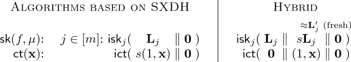
-
If k-Lin holds in the pairing groups, we encode in the secret key k independent copies of label functions \(L_1^t, \dots , L_m^t\) for \(t \in [k]\), and in the ciphertexts k copies of \((1, \mathbf{x})\) multiplied with independent random scalars \(\mathbf{s}[t]\) for \(t\in [k]\). This way, decryption computes a random linear combination of the garblings \((\sum _{t\in [k]}{\mathbf {s}[t]L_1^t(\mathbf{x})},\dots , \sum _{t\in [k]}{\mathbf {s}[t]L_m^t(\mathbf{x})})\) in the exponent, which via a similar hybrid as above corresponds to pseudorandom label functions in the exponent.
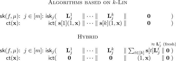
 . As such, decryption computes

The above modification yields a secret-key ABE secure in the many-ciphertext many-key setting. The final hurdle is how to make the scheme public-key, which we resolve using slotted IPFE.
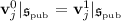
Slotted IPFE. Proposed in [50], slotted IPFE is a hybrid between a secret-key function-hiding IPFE and a public-key IPFE. Here, a vector \(\mathbf{u}\in \mathbb {Z}_p^n\) is divided into two parts \(({\mathbf{u}_\text {pub}, \mathbf{u}_\text {priv}})\) with \(\mathbf {u}_\text {pub}\in \mathbb {Z}_p^{n_\text {pub}}\) in the public slot and \(\mathbf {u}_\text {priv}\in \mathbb {Z}_p^{n_\text {priv}}\) in the private slot (\(n_\text {pub}+n_\text {priv}= n\)). Like a usual secret-key IPFE, the encryption algorithm \(\mathsf {IPFE}.\mathsf {Enc}\) using the master secret key \(\mathsf {msk}\) can encrypt to both the public and private slots, i.e., encrypting any vector \(\mathbf{u}\). In addition, there is an \(\mathsf {IPFE}.\mathsf {SlotEnc}\) algorithm that uses the master public key \(\mathsf {mpk}\), but can only encrypt to the public slot, i.e., encrypting vectors such that \(\mathbf{u}_\text {priv}= \mathbf 0\). Since anyone can encrypt to the public slot, it is impossible to hide the public slot part \(\mathbf{v}_\text {pub}\) of a secret-key vector \(\mathbf{v}\). As a result, slotted IPFE guarantees function-hiding only w.r.t. the private slot, and the weaker indistinguishability security w.r.t. the public slot. Based on the construction of slotted IPFE in [49], we obtain adaptively secure slotted IPFE based on k-Lin.
The aforementioned secret-key ABE scheme can be easily turned into a public-key one with slotted IPFE: The ABE encryption algorithm simply uses \(\mathsf {IPFE}.\mathsf {SlotEnc}\) and \(\mathsf {mpk}\) to encrypt to the public slots. In the security proof, we move vectors encrypted in the public slot of the challenge ciphertext to the private slot, where function-hiding holds and the same security arguments outlined above can be carried out.
Discussion. Our method can be viewed as using IPFE to implement dual system encryption [57]. We believe that IPFE provides a valuable abstraction, making it conceptually simpler to design strategies for moving information between the secret key and the ciphertext, as done in the proof of 1-ABE, and for generating independent randomness, as done in the proof of full ABE. The benefit of this abstraction is even more prominent when it comes to ABE for logspace Turing machines.
2.3 1-ABE for Logspace Turing Machines
We now present ideas for constructing 1-ABE for \(\mathsf {L}\), and then its extension to \(\mathsf {NL}\) and how to handle DFA and NFA as special cases for better efficiency. Moving to full-fledged ABE follows the same ideas in the previous subsection, though slightly more complicated, which we omit in this overview.
1-ABE for \(\mathsf {L}\) enables generating a single secret key \(\mathsf {sk}(M, \mu )\) for a Turing machine M and secret \(\mu \), and a ciphertext \(\mathsf {ct}(\mathbf{x}, T,S)\) specifying an input \(\mathbf{x}\) of length N, a polynomial time bound \(T = \mathrm {poly}({N})\), and a logarithmic space bound \(S = O(\log N)\) such that decryption reveals \(\mu {M}|_{N,T,S} (\mathbf{x})\), where \( {M}|_{N,T,S} (\mathbf{x})\) represents the computation of running \(M(\mathbf{x})\) for T steps with a work tape of size S, which outputs 1 if and only if the computation lands in an accepting state after T steps and has never exceeded the space bound S. A key feature of ABE for uniform computation is that a secret key \(\mathsf {sk}(M, \mu )\) can decrypt ciphertexts with inputs of unbounded lengths and unbounded time/(logarithmic) space bounds. (In contrast, for non-uniform computation, the secret key decides the input length and time/space bounds.) Our 1-ABE for \(\mathsf {L}\) follows the same blueprint of combining AKGS with IPFE, but uses new ideas in order to implement the unique feature of ABE for uniform computation.
Notations for Turing Machines. We start with introducing notations for logspace Turing machines (TM) over the binary alphabet. A TM \(M=({Q, q_\text {acc},\delta })\) consists of Q states, with the initial state being 1 and an accepting stateFootnote 9 \(q_\text {acc}\in [Q]\), and a transition function \(\delta \). The computation of \( {M}|_{N, T,S} (\mathbf{x})\) goes through a sequence of \(T+1\) configurations \((\mathbf{x}, (i, j, \mathbf{W}, q))\), where \(i \in [N]\) is the input tape pointer, \(j \in [S]\) the work tape pointer, \(\mathbf{W} \in {\{{0,1}\}}^S\) the content of the work tape, and \(q \in [Q]\) the state. The initial internal configuration is thus \((i=1,j=1,\mathbf{W} =\mathbf 0_S, q = 1)\), and the transition from one internal configuration \((i, j, \mathbf{W}, q)\) to the next \((i', j', \mathbf{W}', q')\) is governed by the transition function \(\delta \) and the input \(\mathbf{x}\). Namely, if  ,
,

In other words, the transition function \(\delta \) on input state q and bits \(\mathbf{x}[i]\), \(\mathbf{W}[j]\) on the input and work tape under scan, outputs the next state \(q'\), the new bit \(w' \in {\{{0,1}\}}\) to be written to the work tape, and the directions  to move the input and work tape pointers. The next internal configuration is then derived by updating the current configuration accordingly, where \(\mathbf{W}' = \mathsf {overwrite}(\mathbf{W}, j, w')\) is a vector obtained by overwriting the jth cell of \(\mathbf{W}\) with \(w'\) and keeping the other cells unchanged.
AKGS for Logspace Turing Machines. To obtain an AKGS for \(\mathsf {L}\), we represent the TM computation algebraically as a sequence of matrix multiplications over \(\mathbb {Z}_p\), for which we design an AKGS. To do so, we represent each internal configuration as a basis vector \(\mathbf{e}_{(i,j,\mathbf{W},q)}\) of dimension \(NS2^SQ\) with a single 1 at position \((i,j,\mathbf{W}, q)\). We want to find a transition matrix \(\mathbf{M}(\mathbf{x})\) (depending on \(\delta \) and \(\mathbf{x}\)) such that moving to the next state \(\mathbf{e}_{(i', j',\mathbf{W}', q')}\) simply involves (right) multiplying \(\mathbf{M}(\mathbf{x})\), i.e.,  . It is easy to verify that the correct transition matrix is


Here, \(\mathsf {CanTransit}[(i,j,\mathbf{W}),(i' j', \mathbf{W}')]\) indicates whether it is possible, irrespective of \(\delta \), to move from an internal configuration with \((i, j, \mathbf{W})\) to one with \((i', j', \mathbf{W}')\). If possible, then  indicates whether \(\delta \) permits moving from state q with current read bits \(x = \mathbf{x}[i], w= \mathbf{W}[j]\) to state \(q'\) with overwriting bit \(w' = \mathbf{W}'[j]\) and moving directions
  . Armed with this, the TM computation can be done by right multiplying the matrix \(\mathbf{M}(\mathbf{x})\) for T times with the initial configuration
  , reaching the final configuration
  , and then testing whether \(q_T = q_\text {acc}\). More precisely,

To construct AKGS for \(\mathsf {L}\), it boils down to construct AKGS for matrix multiplication. Our construction is inspired by the randomized encoding for arithmetic \(\mathsf {NC}^1\) scheme of [11] and the garbling mechanism for multiplication gates in [19]. Let us focus on garbling the computation \( {M}|_{N,T,S} (\mathbf{x})\) with secrets \(\alpha = \mu \) and \(\beta = 0\) (the case needed in our 1-ABE). The garbling algorithm \(\mathsf {Garble}\) produces the following affine label functions of \(\mathbf{x}\):

Here, \(z=(i,j,\mathbf {W},q)\) runs through all \(NS2^SQ\) possible internal configurations and  . The evaluation proceeds inductively, starting with
  , going through
  for every \(t \in [T]\) using the identity below, and completing after T steps by combining
  with \(\varvec{\ell }_{T+1}\) to get
  as desired:

We now show that the above AKGS is piecewise secure. First, \(\ell _\text {init}\) is reversely sampleable. Since \(\mathsf {Eval}\) is linear in the labels and \(\ell _\text {init}\) has coefficient 1, given all but the first label \(\ell _\text {init}\), one can reversely sample \(\ell _\text {init}\), the value uniquely determined by the linear equationFootnote 10 imposed by the correctness of \(\mathsf {Eval}\). Second, the marginal randomness property holds because every label \(\varvec{\ell }_t\) is random due to the random additive term \(\mathbf{r}_{t-1}\) that is not used in subsequent label functions \(L_{t',z}\) for all \(t'>t\) and z, nor in the non-constant terms of \(L_{t,z}\)’s—we call \(\mathbf{r}_{t-1}\) the randomizers of \(\varvec{\ell }_t\) (highlighted in the box). Lastly, we observe that the size of the garbling is \((T+1)NS2^SQ + 1\).
1-ABE for \({\varvec{\mathsf {L}}}\). We now try to construct 1-ABE for \(\mathsf {L}\) from AKGS for \(\mathsf {L}\), following the same blueprint of using IPFE. Yet, applying the exact same method for non-uniform computation fails for multiple reasons. In 1-ABE for non-uniform computation, the ciphertext \(\mathsf {ct}\) contains a single IPFE ciphertext \(\mathsf {ict}\) encoding \((1, \mathbf{x})\), and the secret key \(\mathsf {sk}\) contains a set of IPFE secret keys \(\mathsf {isk}_j\) encoding all the label functions. However, in the uniform setting, the secret key \(\mathsf {sk}(M, \mu )\) depends only on the TM M and the secret \(\mu \), and is supposed to work with ciphertexts \(\mathsf {ct}(\mathbf{x}, T,S)\) with unbounded \(N=|\mathbf{x}|, T, S\). Therefore, at key generation time, the size of the AKGS garbling, \((T+1)NS2^SQ + 1\), is unknown, let alone generating and encoding all the label functions. Moreover, we want our 1-ABE to be compact, with secret key size \(|\mathsf {sk}| = O(Q)\) linear in the number Q of states and ciphertext size \(|\mathsf {ct}| = O(TNS2^S)\) (ignoring polynomial factors in the security parameter). The total size of secret key and ciphertext is much smaller than the total number of label functions, i.e., \( |\mathsf {sk}|+|\mathsf {ct}| \ll (T+1)NS2^SQ + 1\).
To overcome these challenges, our idea is that instead of encoding the label functions in the secret key or the ciphertext (for which there is not enough space), we let the secret key and the ciphertext jointly generate the label functions. For this idea to work, the label functions cannot be generated with true randomness which cannot be “compressed”, and must use pseudorandomness instead. More specifically, our 1-ABE secret key \(\mathsf {sk}(M,\mu )\) contains \(\sim Q\) IPFE secret keys \(\{\mathsf {isk}(\mathbf{v}_j)\}_j\), while the ciphertext \(\mathsf {ct}(\mathbf{x}, T, S)\) contains \(\sim TNS2^S\) IPFE ciphertexts \(\{\mathsf {ict}(\mathbf{u}_i)\}_i\), such that decryption computes in the exponent \(\sim TNS2^SQ\) cross inner products \(\langle \mathbf{u}_i, \mathbf{v}_j\rangle \) that correspond to a garbling of \( {M}|_{N,T,S} (\mathbf{x})\) with secret \(\mu \). To achieve this, we rely crucially on the special block structure of the transition matrix \(\mathbf{M}\) (which in turn stems from the structure of TM computation, where the same transition function is applied in every step). Furthermore, as discussed above, we replace every truly random value \(\mathbf{r}_t[i,j,\mathbf{W},q]\) with a product \(\mathbf {r}_\mathrm {x}[t,i,j,\mathbf{W}]\mathbf {r}_\mathrm {f}[q]\), which can be shown pseudorandom in the exponent based on SXDH.Footnote 11
 Let us examine the transition matrix again (cf. Eqs. (4) and (5)):
We see that that every block  either is the \(Q\times Q\) zero matrix or belongs to a small set \(\mathcal T\) of a constant number of transition blocks:

Moreover, in the \(\mathfrak {i}= (i,j,\mathbf {W})\)th “block row”,  , each transition block
  either does not appear at all if \(x\ne \mathbf{x}[i]\) or \(w' \ne \mathbf{W}[j]\), or appears once as the block
  , where \(\mathfrak {i}'\) is the triplet obtained by updating \(\mathfrak {i}\) appropriately according to
  :
:

Thus we can “decompose” every label \(\varvec{\ell }_t[\mathfrak {i},q]\) as an inner product \(\langle \mathbf {u}_{t,\mathfrak {i}},\mathbf {v}_q\rangle \) as

where vectors \(\mathbf {u}_{t,\mathfrak {i}}\) and \(\mathbf {v}_q\) are as follows, with \(\mathbbm {1}\{{\cdots }\}\) indicating if the conditions (its argument) are true:

Similarly, we can “decompose”  as \( \langle \mathbf {r}_\mathrm {x}[0,1,1,\mathbf 0],\mathbf {r}_\mathrm {f}[1]\rangle \). (For simplicity in the discussion below, we omit details on how to handle \(\varvec{\ell }_{T+1}\).) Given such decomposition, our semi-compact 1-ABE scheme follows immediately by using IPFE to compute the garbling:
Honest Algorithms
Decrypting the pair \(\mathsf {isk}_\text {init}, \mathsf {ict}_\text {init}\) (generated using one master secret key) gives exactly the first label \(\ell _\text {init}\), while decrypting \(\mathsf {isk}_q, \mathsf {ict}_{t,\mathfrak {i}}\) (generated using another master secret key) gives the label \(\varvec{\ell }_{t}[\mathfrak {i},q]\) in the exponent, generated using pseudorandomness \(\mathbf {r}_t[\mathfrak {i},q] = \mathbf {r}_\mathrm {x}[t,\mathfrak {i}]\mathbf {r}_\mathrm {f}[q]\). Note that the honest algorithms encode \(\mathbf {r}_\mathrm {f}[q]\) (in \(\mathbf {v}_q\)) and \(\mathbf {r}_\mathrm {x}[t,\mathfrak {i}]\) (in \(\mathbf {u}_{t,\mathfrak {i}}\)) in IPFE secret keys and ciphertexts that use the two source groups \(G_1\) and \(G_2\) respectively. As such, we cannot directly use the SXDH assumption to argue the pseudorandomness of \(\mathbf {r}_t[\mathfrak {i},q]\). In the security proof, we will use the function-hiding property of IPFE to move both \(\mathbf {r}_\mathrm {x}[t,\mathfrak {i}]\) and \(\mathbf {r}_\mathrm {f}[q]\) into the same source group before invoking SXDH.
Adaptive Security. To show adaptive security, we follow the same blueprint of going through a sequence of hybrids, where we first hardcode \(\ell _\text {init}\) and sample it reversely using \(\mathsf {RevSamp}\), and next simulate the other labels \(\varvec{\ell }_t[\mathfrak {i},q]\) one by one. Hardwiring \(\ell _\text {init}\) is easy by relying on the function-hiding property of IPFE. However, it is now more difficult to simulate \(\varvec{\ell }_t[\mathfrak {i},q]\) because (i) before simulating \(\varvec{\ell }_t[\mathfrak {i},q]\), we need to switch its randomizer \(\mathbf {r}_{t-1}[\mathfrak {i},q] = \mathbf {r}_\mathrm {x}[t-1,\mathfrak {i}]\mathbf {r}_\mathrm {f}[q]\) to truly random  , which enables us to simulate the label \(\varvec{\ell }_t[\mathfrak {i},q]\) as random; and (ii) to keep simulation progressing, we need to switch the random \(\varvec{\ell }_t[\mathfrak {i},q]\) back to a pseudorandom value \(\varvec{\ell }_t[\mathfrak {i},q] = \mathbf {s}_\mathrm {x}[t,\mathfrak {i}]\mathbf {s}_\mathrm {f}[q]\), as otherwise, there is not enough space to store all \(\sim TNS2^SQ\) random labels \(\varvec{\ell }_t[\mathfrak {i},q]\).
We illustrate how to carry out above proof steps in the simpler case where the adversary queries for the ciphertext first and the secret key second. The other case where the secret key is queried first is handled using similar ideas, but the technicality becomes much more delicate.
In hybrid \((t,\mathfrak {i})\), the first label \(\ell _\text {init}\) is reversely sampled and hardcoded in the secret key \(\mathsf {isk}_\text {init}\), i.e., \(\mathsf {ict}_\text {init}\) encrypts \(({1\parallel 0})\) and \(\mathsf {isk}_\text {init}\) encrypts \(({\ell _\text {init}\parallel 0})\) with \(\ell _\text {init}\leftarrow \mathsf {RevSamp}({\cdots })\). All labels \(\varvec{\ell }_{t'}[\mathfrak {i}',q]\) with \((t',\mathfrak {i}') < (t, \mathfrak {i})\) have been simulated as \(\mathbf {s}_\mathrm {x}[t',\mathfrak {i}']\mathbf {s}_\mathrm {f}[q]\)—observe that the ciphertext \(\mathsf {ict}_{t',\mathfrak {i}'}\) encodes only \(\mathbf {s}_\mathrm {f}[t',\mathfrak {i}']\) in the second slot, which is multiplied by \(\mathbf {s}_\mathrm {f}[q]\) in the second slot of \(\mathsf {isk}_q\). On the other hand, all labels \(\varvec{\ell }_{t'}[\mathfrak {i}',q]\) with \((t',\mathfrak {i}') \ge (t, \mathfrak {i})\) are generated honestly as the honest algorithms do.

Moving from hybrid \((t,\mathfrak {i})\) to its successor \((t,\mathfrak {i})+1\), the only difference is that labels \(\varvec{\ell }_t[\mathfrak {i},q]\) are switched from being honestly generated \(\langle \mathbf {u}_{t,\mathfrak {i}}, \mathbf {v}_q \rangle \) to pseudorandom \(\mathbf {s}_\mathrm {x}[t,\mathfrak {i}]\mathbf {s}_\mathrm {f}[q]\), as depicted above with values in the solid line box (the rest of the hybrid is identical to hybrid \((t,\mathfrak {i})\)). The transition can be done via an intermediate hybrid \((t,\mathfrak {i}):1\) with values in the dash line box. In this hybrid, all labels \(\varvec{\ell }_t[\mathfrak {i},q]\) produced as inner products of all \(\mathbf {v}_q\)’s and \(\mathbf {u}_{t,\mathfrak {i}}\) are temporarily hardcoded in the secret keys \(\mathsf {isk}_q\), using the third slot (which is zeroed out in all the other \(\mathbf {u}_{(t',\mathfrak {i}')\ne (t,\mathfrak {i})}\)’s). Furthermore, \(\mathbf {u}_{t,\mathfrak {i}}\) is removed from \(\mathsf {ict}_{t,\mathfrak {i}}\). As such, the random scalar \(\mathbf {r}_\mathrm {x}[t-1,\mathfrak {i}]\) (formerly embedded in \(\mathbf {u}_{t,\mathfrak {i}}\)) no longer appears in the exponent of group \(G_1\), and \(\ell _\text {init}\leftarrow \mathsf {RevSamp}({\cdots })\) can be performed using \(\mathbf {r}_\mathrm {x}[{t-1,\mathfrak {i}}], \mathbf {r}_\mathrm {f}[q], \mathbf {r}_{t-1}[{\mathfrak {i},q}]\) in the exponent of \(G_2\). Therefore, we can invoke the SXDH assumption in \(G_2\) to switch the randomizers \(\mathbf {r}_{t-1}[\mathfrak {i},q] = \mathbf {r}_\mathrm {x}[t-1,\mathfrak {i}]\mathbf {r}_\mathrm {f}[q]\) to be truly random, and hence so are the labels  . By a similar argument, this intermediate hybrid \((t,\mathfrak {i}):1\) is also indistinguishable to \((t,\mathfrak {i})+1\), as the random \(\varvec{\ell }_t[\mathfrak {i},q]\) can be switched to \(\mathbf {s}_\mathrm {x}[t,\mathfrak {i}]\mathbf {s}_\mathrm {f}[q]\) in hybrid \((t,\mathfrak {i})+1\), relying again on SXDH and the function-hiding property of IPFE. This concludes our argument of security in the simpler case where the ciphertext is queried first.
AKGS and 1-ABE for \({{\mathsf {NL}}}\). Our construction of AKGS and 1-ABE essentially works for \(\mathsf {NL}\) without modification, because the computation of a non-deterministic logspace Turing machine \(M = ([Q],q_\text {acc},\delta )\) on an input \(\mathbf {x}\) can also be represented as a sequence of matrix multiplications. We briefly describe how by pointing out the difference from \(\mathsf {L}\). The transition function \(\delta \) of a non-deterministic TM dost not instruct a unique transition, but rather specifies a set of legitimate transitions. Following one internal configuration \((i,j,\mathbf {W},q)\), there are potentially many legitimate successors:

The computation is accepting if and only if there exists a path with T legitimate transitions starting from \((1,1,\mathbf 0, 1)\), through \((i_t,j_t,\mathbf {W}_t, q_t)\) for \(t \in [T]\), and landing at \(q_T =q_\text {acc}\).
Naturally, we modify the transition matrix as below to reflect all legitimate transitions. The only difference is that each transition block determined by \(\delta \) may map a state q to multiple states \(q'\), as highlighted in the solid line box:

Let us observe the effect of right multiplying \(\mathbf {M}(\mathbf {x})\) to an \(\mathbf {e}_{\mathfrak {i},q}\) indicating configuration \((\mathfrak {i},q)\):  gives a vector \(\mathbf {c}_1\) such that \(\mathbf {c}_1[\mathfrak {i}',q'] = 1\) if and only if \((\mathfrak {i}',q')\) is a legitimate next configuration. Multiplying \(\mathbf {M}(\mathbf {x})\) one more time,
  gives \(\mathbf {c}_2\) where \(\mathbf {c}_2[\mathfrak {i}',q']\) is the number of length-2 paths of legitimate transitions from \((\mathfrak {i},q)\) to \((\mathfrak {i}',q')\). Inductively,
  yields \(\mathbf {c}_t\) that counts the number of length-t paths from \((\mathfrak {i},q)\) to any other internal configuration \((\mathfrak {i}',q')\). Therefore, we can arithmetize the computation of M on \(\mathbf{x}\) as

Right multiplying \(\mathbf{t}\) in the end sums up the number of paths to \((\mathfrak {i},q_\text {acc})\) for all \(\mathfrak {i}\) in \(\mathbf {c}_T\) (i.e., accepting paths).
If the computation is not accepting—there is no path to any \((\mathfrak {i}, q_\text {acc})\)—the final sum would be 0 as desired. If the computation is accepting—there is a path to some \((\mathfrak {i}, q_\text {acc})\)—then the sum should be non-zero (up to the following technicality). Now that we have represented \(\mathsf {NL}\) computation as matrix multiplication, we immediately obtain AKGS and 1-ABE for \(\mathsf {NL}\) using the same construction for \(\mathsf {L}\).
 The correctness of our scheme relies on the fact that when the computation is accepting, the matrix multiplication formula (Eq. (6)) counts correctly the total number of length-T accepting paths. However, a subtle issue is that in our 1-ABE, the matrix multiplications are carried out over \(\mathbb {Z}_p\), where p is the order of the bilinear pairing groups. This means if the total number of accepting paths happens to be a multiple of p, the sequence of matrix multiplications mod p carried out in 1-ABE would return 0, while the correct output should be non-zero. This technicality can be circumvented if p is entropic with \(\omega (\log n)\) bits of entropy and the computation \((M, \mathbf{x}, T,S)\) is independent of p. In that case, the probability that the number of accepting paths is a multiple of p is negligible. We can achieve this by letting the setup algorithm of 1-ABE sample the bilinear pairing groups from a distribution with entropic order. Then, we have statistical correctness for computations \((M, \mathbf{x}, T,S)\) chosen statically ahead of time (independent of p). We believe such static correctness is sufficient for most applications where correctness is meant for non-adversarial behaviors. However, if the computation \((M, \mathbf{x}, T,S)\) is chosen adaptively to make the number of accepting paths a multiple of p, then an accepting computation will be mistakenly rejected. We stress that security is unaffected since if an adversary chooses M and \((\mathbf{x}, T,S)\) as such, it only learns less information.
The Special Cases of DFA and NFA. DFA and NFA are special cases of \(\mathsf {L}\) and \(\mathsf {NL}\), respectively, as they can be represented as Turing machines with a work tape of size \({S=1}\) that always runs in time \({T=N}\), and the transition function \(\delta \) always moves the input tape pointer to the right. Therefore, the internal configuration of a finite automaton contains only the state q, and the transition matrix \(\mathbf {M}(x)\) is determined by \(\delta \) and the current input bit x under scan. Different from the case of \(\mathsf {L}\) and \(\mathsf {NL}\), here the transition matrix no longer keeps track of the input tape pointer since its move is fixed—the tth step uses the transition matrix \(\mathbf {M}(\mathbf {x}[t])\) depending on \(\mathbf {x}[t]\). Thus, the computation can be represented as follows:

Our construction of AKGS directly applies:

When using pseudorandomness \(\mathbf{r}_t[q] = \mathbf {r}_\mathrm {f}[q]\mathbf {r}_\mathrm {x}[t]\), the labels \(\varvec{\ell }_t[q]\) can be computed as the inner products of \(\mathbf {v}_q = (-\mathbf {r}_\mathrm {f}[q] \parallel (\mathbf {M}_0 \mathbf {r}_\mathrm {f})[q] \parallel (\mathbf {M}_1\mathbf {r}_\mathrm {f})[q] \parallel \mathbf 0)\) and \(\mathbf {u}_t=(\mathbf {r}_\mathrm {x}[t-1]\parallel (1-\mathbf {x}[t]) \mathbf {r}_\mathrm {x}[t]\parallel \mathbf {x}[t] \mathbf {r}_\mathrm {x}[t]\parallel \mathbf 0)\). Applying our 1-ABE construction with respect to such “decomposition” gives compact 1-ABE for DFA and NFA with secret keys of size O(Q) and ciphertexts of size O(N).
Discussion. Prior to our work, there have been constructions of ABE for DFA based on pairing [1, 5, 12, 13, 29, 58] and ABE for NFA based on LWE [4]. However, no previous scheme achieves adaptive security unless based on q-type assumptions [12, 13]. The work of [20] constructed ABE for DFA, and that of [7] for random access machines, both based on LWE, but they only support inputs of bounded length, giving up the important advantage of uniform computation of handling unbounded-length inputs. There are also constructions of ABE (and even the stronger generalization, functional encryption) for Turing machines [3, 9, 28, 41] based on strong primitives such as multilinear map, extractable witness encryption, and indistinguishability obfuscation. However, these primitives are non-standard and currently not well-understood.
In terms of techniques, our work is most related to previous pairing-based ABE for DFA, in particular, the recent construction based on k-Lin [29]. These ABE schemes for DFA use a linear secret-sharing scheme for DFA first proposed in [58], and combining the secret key and ciphertext produces a secret-sharing in the exponent, which reveals the secret if and only if the DFA computation is accepting. Proving (even selective) security is complicated. Roughly speaking, the work of [29] relies on an entropy propagation technique to trace the DFA computation and propagate a few random masks “down” the computation path, with which they can argue that secret information related to states that are backward reachable from the final accepting states is hidden. The technique is implemented using the “nested two-slot” dual system encryption [23, 33, 46, 47, 54, 57] combined with a combinatorial mechanism for propagation.
Our AKGS is a generalization of Waters’ secret-sharing scheme to \(\mathsf {L}\) and \(\mathsf {NL}\), and the optimized version for DFA is identical to Waters’ secret-sharing scheme. Furthermore, our 1-ABE scheme from AKGS and IPFE is more modular. In particular, our proof (similar to our 1-ABE for non-uniform computation) does not reason about or trace the computation, and simply relies on the structure of AKGS. Using IPFE enables us to design sophisticated sequences of hybrids without getting lost in the algebra, as IPFE helps separating the logic of changes in different hybrids from how to implement the changes. For instance, we can easily manage multiple slots in the vectors encoded in IPFE for holding temporary values and generating pseudorandomness.
3 Preliminaries
Indexing. Let S be any set, we write \(S^\mathcal {I}\) for the set of vectors whose entries are in S and indexed by \(\mathcal {I}\), i.e., \(S^\mathcal {I}=\{{(\mathbf {v}[i])_{i\in \mathcal {I}}}{\,|\,}{\mathbf {v}[i]\in S}\}\). Suppose  are two index sets with
  . For any vector
  , we write
  for its zero-extension into
  , i.e.,
  and \(\mathbf {u}[i]=\mathbf {v}[i]\) if
  and 0 otherwise. Conversely, for any vector
  , we write
  for its canonical projection onto
  , i.e.,
  and \(\mathbf {u}[i]=\mathbf {v}[i]\) for
  . Lastly, let
  , denote by \(\langle {\mathbf {u},\mathbf {v}}\rangle \) their inner product, i.e.,
  .
.
Coefficient Vector. We conveniently associate an affine function \(f:\mathbb {Z}_p^\mathcal {I}\rightarrow \mathbb {Z}_p\) with its coefficient vector  (written as the same letter in boldface) for
  such that \(f(\mathbf {x})=\mathbf {f}[\mathsf {const}]+\sum _{i\in \mathcal {I}}{\mathbf {f}[\mathsf {coef}_i]\mathbf {x}[i]}\).
3.1 Bilinear Pairing and Matrix Diffie-Hellman Assumption
Throughout the paper, we use a sequence of bilinear pairing groups
where \(G_{\lambda ,1},G_{\lambda ,2},G_{\lambda ,\text {T}}\) are groups of prime order \(p=p(\lambda )\), and \(G_{\lambda ,1}\) (resp. \(G_{\lambda ,2}\)) is generated by \(g_{\lambda ,1}\) (resp. \(g_{\lambda ,2}\)). The maps \(e_\lambda :G_{\lambda ,1}\times G_{\lambda ,_2}\rightarrow G_{\lambda ,\text {T}}\) are
-
bilinear: \(e_\lambda (g_{\lambda ,1}^a,g_{\lambda ,2}^b)=\bigl (e_\lambda ({g_{\lambda ,1},g_{\lambda ,2}})\bigr )^{ab}\) for all a, b; and
-
non-degenerate: \(e_\lambda ({g_{\lambda ,1},g_{\lambda ,2}})\) generates \(G_{\lambda ,\text {T}}\).
Implicitly, we set \(g_{\lambda ,\text {T}}=e({g_{\lambda ,1},g_{\lambda ,2}})\). We require the group operations as well as the bilinear maps be efficiently computable.
Bracket Notation. Fix a security parameter, for \(i=1,2,\text {T}\), we write \( \mathopen [\!\mathopen [{\mathbf {A}}\mathclose ]\!\mathclose ] _i\) for \(g_{\lambda ,i}^{\mathbf {A}}\), where the exponentiation is element-wise. When bracket notation is used, group operation is written additively, so \( \mathopen [\!\mathopen [{\mathbf {A}+\mathbf {B}}\mathclose ]\!\mathclose ] _i= \mathopen [\!\mathopen [{\mathbf {A}}\mathclose ]\!\mathclose ] _i+ \mathopen [\!\mathopen [{\mathbf {B}}\mathclose ]\!\mathclose ] _i\) for matrices \(\mathbf {A},\mathbf {B}\). Pairing operation is written multiplicatively so that \( \mathopen [\!\mathopen [{\mathbf {A}}\mathclose ]\!\mathclose ] _1 \mathopen [\!\mathopen [{\mathbf {B}}\mathclose ]\!\mathclose ] _2= \mathopen [\!\mathopen [{\mathbf {A}\mathbf {B}}\mathclose ]\!\mathclose ] _\text {T}\). Furthermore, numbers can always operate with group elements, e.g., \( \mathopen [\!\mathopen [{\mathbf {A}}\mathclose ]\!\mathclose ] _1\mathbf {B}= \mathopen [\!\mathopen [{\mathbf {A}\mathbf {B}}\mathclose ]\!\mathclose ] _1\).
Matrix Diffie-Hellman Assumption. In this work, we rely on the MDDH assumptions defined in [26], which is implied by k-Lin.
Definition 1
(\(\text {MDDH}_k\) [26]). Let \(k\ge 1\) be an integer constant. For a sequence of pairing groups \(\mathcal {G}\) of order \(p(\lambda )\), \(\text {MDDH}_k\) holds in \(G_i\) (\(i=1,2,\text {T}\)) if

3.2 Attribute-Based Encryption
Definition 2
Let \(\mathcal {M}=\{M_\lambda \}_{\lambda \in \mathbb {N}}\) be a sequence of message sets. Let \(\mathcal {P}=\{\mathcal {P}_\lambda \}_{\lambda \in \mathbb {N}}\) be a sequence of families of predicates, where \(\mathcal {P}_\lambda =\{{P:X_P\times Y_P\rightarrow {\{{0,1}\}}}\}\). An attribute-based encryption (ABE) scheme for message space \(\mathcal {M}\) and predicate space \(\mathcal {P}\) consists of 4 efficient algorithms:
-
\(\mathsf {Setup}({1^\lambda ,P\in \mathcal {P}_\lambda })\) generates a pair of master public/secret key \(({\mathsf {mpk},\mathsf {msk}})\).
-
\(\mathsf {KeyGen}({1^\lambda ,\mathsf {msk},y\in Y_P})\) generates a secret key \(\mathsf {sk}_y\) associated with y.
-
\(\mathsf {Enc}({1^\lambda ,\mathsf {mpk},x\in X_P,g\in M_\lambda })\) generates a ciphertext \(\mathsf {ct}_{x,g}\) for g associated with x.
-
\(\mathsf {Dec}({1^\lambda ,\mathsf {sk},\mathsf {ct}})\) outputs either \(\bot \) or a message in \(M_\lambda \).
Correctness requires that for all \(\lambda \in \mathbb {N}\), all \(P\in \mathcal {P}_\lambda ,g\in M_\lambda \), and all \({y\in Y_P}, {x\in X_P}\) such that \({P({x,y})=1}\),

The basic security requirement of an ABE scheme stipulates that no information about the message can be inferred as long as each individual secret key the adversary receives does not allow decryption. The adversary is given the master public key and allowed arbitrarily many secret key and ciphertexts queries. For the secret key queries, the adversary is given the secret key for a policy of its choice. For the ciphertext queries, the adversary is either given a correct encryption to the message or an encryption of a random message. It has to decide whether the encryptions it receives are correct or random. We stress that in the adaptive setting considered in this work, the secret key and ciphertext queries can arbitrarily interleave and depend on responses to previous queries. The definition is standard in the literature, and we refer the readers to [32] or the full version for details.
3.3 Function-Hiding Slotted Inner-Product Functional Encryption
Definition 3
(pairing-based slotted IPFE). Let \(\mathcal {G}\) be a sequence of pairing groups of order \(p(\lambda )\). A slotted inner-product functional encryption (IPFE) scheme based on \(\mathcal {G}\) consists of 5 efficient algorithms:
-
 takes as input two disjoint index sets, the public slot
  and the private slot
  , and outputs a pair of master public key and master secret key \(({\mathsf {mpk},\mathsf {msk}})\). The whole index set
  is
is  .
. -
\(\mathsf {KeyGen}({1^\lambda ,\mathsf {msk}, \mathopen [\!\mathopen [{\mathbf {v}}\mathclose ]\!\mathclose ] _2})\) generates a secret key \(\mathsf {sk}_{\mathbf {v}}\) for
 .
. -
\(\mathsf {Enc}({1^\lambda ,\mathsf {msk}, \mathopen [\!\mathopen [{\mathbf {u}}\mathclose ]\!\mathclose ] _1})\) generates a ciphertext \(\mathsf {ct}_{\mathbf {u}}\) for
 using the master secret key.
 -
\(\mathsf {Dec}({1^\lambda ,\mathsf {sk}_{\mathbf {v}},\mathsf {ct}_{\mathbf {u}}})\) is supposed to compute \( \mathopen [\!\mathopen [{\langle \mathbf {u},\mathbf {v}\rangle }\mathclose ]\!\mathclose ] _\text {T}\).
-
\(\mathsf {SlotEnc}({1^\lambda ,\mathsf {mpk}, \mathopen [\!\mathopen [{\mathbf {u}}\mathclose ]\!\mathclose ] _1})\) generates a ciphertext \(\mathsf {ct}\) for
 when given input
  using the master public key.
 takes as input two disjoint index sets, the public slot
  and the private slot
  , and outputs a pair of master public key and master secret key
  is
is  .
. .
. using the master secret key.
 when given input
  using the master public key.
Decryption correctness requires that for all \(\lambda \in \mathbb {N}\), all index set  , and all vectors
  ,
,

Slot-mode correctness requires that for all \(\lambda \in \mathbb {N}\), all disjoint index sets  , and all vector
  , the following distributions should be identical:

Slotted IPFE generalizes both secret-key and public-key IPFEs: A secret-key IPFE can be obtained by setting  and
and  ; a public-key IPFE can be obtained by setting
  and
and  .
.
We now define the adaptive function-hiding property.
Definition 4
(function-hiding slotted IPFE). Let \(({\mathsf {Setup},\mathsf {KeyGen},\mathsf {Enc},\mathsf {Dec},}\) \({\mathsf {SlotEnc}})\) be a slotted IPFE. The scheme is function-hiding if \(\mathsf {Exp}_\text {FH}^0\approx \mathsf {Exp}_\text {FH}^1\), where \(\mathsf {Exp}_\text {FH}^b\) for \(b\in {\{{0,1}\}}\) is defined as follows:
-
Setup. Run the adversary \(\mathcal {A}(1^\lambda )\) and receive two disjoint index sets
 from \(\mathcal {A}\). Let
  . Run
. Run  and return \(\mathsf {mpk}\) to \(\mathcal {A}\).
 -
Challenge. Repeat the following for arbitrarily many rounds determined by \(\mathcal {A}\): In each round, \(\mathcal {A}\) has 2 options.
-
\(\mathcal {A}\) can submit \( \mathopen [\!\mathopen [{\mathbf {v}_j^0}\mathclose ]\!\mathclose ] _2, \mathopen [\!\mathopen [{\mathbf {v}_j^1}\mathclose ]\!\mathclose ] _2\) for a secret key, where
 . Upon this query, run
  and return \(\mathsf {sk}_j\) to \(\mathcal {A}\).
 -
\(\mathcal {A}\) can submit \( \mathopen [\!\mathopen [{\mathbf {u}_i^0}\mathclose ]\!\mathclose ] _1, \mathopen [\!\mathopen [{\mathbf {u}_i^1}\mathclose ]\!\mathclose ] _1\) for a ciphertext, where
 . Upon this query, run
  and return \(\mathsf {ct}_i\) to \(\mathcal {A}\).
-
-
Guess. \(\mathcal {A}\) outputs a bit \(b'\). The outcome is \(b'\) if
 for all j and \(\langle {\mathbf {u}_i^0,\mathbf {v}_j^0}\rangle =\langle {\mathbf {u}_i^1,\mathbf {v}_j^1}\rangle \) for all i, j. Otherwise, the outcome is 0.
 from
from  . Run
. Run  and return
  . Upon this query, run
  and return
  . Upon this query, run
  and return
  for all j and
 Applying the techniques in [49, 50] to the IPFE of [2, 60], we obtain adaptively secure function-hiding slotted IPFE:
Lemma 5
([2, 49, 50, 60]). Let \(\mathcal {G}\) be a sequence of pairing groups and \(k\ge 1\) an integer constant. If \(\text {MDDH}_k\) holds in both \(G_1,G_2\), then there is an (adaptively) function-hiding slotted IPFE scheme based on \(\mathcal {G}\).
4 Arithmetic Key Garbling Scheme
Arithmetic key garbling scheme (AKGS) is an information-theoretic primitive related to randomized encodings [11] and partial garbling schemes [37]. It is the information-theoretic core in our construction of one-key one-ciphertext ABE (more precisely 1-ABE constructed in Sect. 5). Given a function \(f:\mathbb {Z}_p^\mathcal {I}\rightarrow \mathbb {Z}_p\) and two secrets \(\alpha ,\beta \in \mathbb {Z}_p\), an AKGS produces label functions \(L_1,\dots ,L_m:\mathbb {Z}_p^\mathcal {I}\rightarrow \mathbb {Z}_p\) that are affine in \(\mathbf {x}\). For any \(\mathbf {x}\), one can compute \(\alpha f(\mathbf {x})+\beta \) from \(L_1(\mathbf {x}),\dots ,L_m(\mathbf {x})\) together with f and \(\mathbf {x}\), while all other information about \(\alpha ,\beta \) are hidden.
Definition 6
(AKGS, adopted from Definition 1 in [37]). An arithmetic key garbling scheme (AKGS) for a function class \(\mathcal {F}=\{f\}\), where \(f:\mathbb {Z}_p^\mathcal {I}\rightarrow \mathbb {Z}_p\) for some \(p,\mathcal {I}\) specified by f, consists of two efficient algorithms:
-
\(\mathsf {Garble}({f\in \mathcal {F},\alpha \in \mathbb {Z}_p,\beta \in \mathbb {Z}_p})\) is randomized and outputs m affine functions \(L_1,\dots ,L_m:\mathbb {Z}_p^\mathcal {I}\rightarrow \mathbb {Z}_p\) (called label functions, which specifies how input is encoded as labels). Pragmatically, it outputs the coefficient vectors \(\mathbf {L}_1,\dots ,\mathbf {L}_m\).
-
\(\mathsf {Eval}({f\in \mathcal {F},\mathbf {x}\in \mathbb {Z}_p^\mathcal {I},\ell _1\in \mathbb {Z}_p,\dots ,\ell _m\in \mathbb {Z}_p})\) is deterministic and outputs a value in \(\mathbb {Z}_p\) (the input \(\ell _1,\dots ,\ell _m\) are called labels, which are supposed to be the values of the label functions at \(\mathbf {x}\)).
Correctness requires that for all \(f:\mathbb {Z}_p^\mathcal {I}\rightarrow \mathbb {Z}_p\in \mathcal {F},\alpha ,\beta \in \mathbb {Z}_p,\mathbf {x}\in \mathbb {Z}_p^\mathcal {I}\),

We also require that the scheme have deterministic shape, meaning that m is determined solely by f, independent of \(\alpha ,\beta \), and the randomness in \(\mathsf {Garble}\). The number of label functions, m, is called the garbling size of f under this scheme.
Definition 7
(linear AKGS). An AKGS \(({\mathsf {Garble},\mathsf {Eval}})\) for \(\mathcal {F}\) is linear if the following conditions hold:
-
\(\mathsf {Garble}({f,\alpha ,\beta })\) uses a uniformly random vector
 as its randomness, where \(m'\) is determined solely by f, independent of \(\alpha ,\beta \).
 -
The coefficient vectors \(\mathbf {L}_1,\dots ,\mathbf {L}_m\) produced by \(\mathsf {Garble}({f,\alpha ,\beta ;\mathbf {r}})\) are linear in \(({\alpha ,\beta ,\mathbf {r}})\).
-
\(\mathsf {Eval}({f,\mathbf {x},\ell _1,\dots ,\ell _m})\) is linear in \(({\ell _1,\dots ,\ell _m})\).
 as its randomness, where
 Later in this paper, AKGS refers to linear AKGS by default.
The basic security notion of AKGS requires the existence of an efficient simulator that draws a sample from the real labels’ distribution given \(f,\mathbf {x},\alpha f(\mathbf {x})+\beta \). We emphasize, as it’s the same case in [37], that AKGS does not hide \(\mathbf {x}\) and hides all other information about \(\alpha ,\beta \) except the value \(\alpha f(\mathbf {x})+\beta \).
Definition 8
((usual) simulation security, Definition 1 in [37]). An AKGS \(({\mathsf {Garble},\mathsf {Eval}})\) for \(\mathcal {F}\) is secure if there exists an efficient algorithm \(\mathsf {Sim}\) such that for all \(f:\mathbb {Z}_p^\mathcal {I}\rightarrow \mathbb {Z}_p\in \mathcal {F},\alpha ,\beta \in \mathbb {Z}_p,\mathbf {x}\in \mathbb {Z}_p^\mathcal {I}\), the following distributions are identical:

As discussed in Sect. 2.1, the usual simulation security suffices for selective (or semi-adaptive) security. To achieve adaptive security, we need the following stronger property.
Definition 9
(piecewise security). An AKGS \(({\mathsf {Garble},\mathsf {Eval}})\) for \(\mathcal {F}\) is piecewise secure if the following conditions hold:
-
The first label is reversely sampleable from the other labels together with f and \(\mathbf {x}\). This reconstruction is perfect even given all the other label functions. Formally, there exists an efficient algorithm \(\mathsf {RevSamp}\) such that for all \({f:\mathbb {Z}_p^\mathcal {I}\rightarrow \mathbb {Z}_p}\in \mathcal {F},{\alpha ,\beta \in \mathbb {Z}_p},{\mathbf {x}\in \mathbb {Z}_p^\mathcal {I}}\), the following distributions are identical:

-
For the other labels, each is marginally random even given all the label functions after it. Formally, this means for all \({f:\mathbb {Z}_p^\mathcal {I}\rightarrow \mathbb {Z}_p\in \mathcal {F}}, {\alpha ,\beta \in \mathbb {Z}_p}, {\mathbf {x}\in \mathbb {Z}_p^\mathcal {I}}\) and all \({j\in [m],j>1}\), the following distributions are identical:


As piecewise security is stronger, it implies the usual simulation security:
Lemma 10
A piecewise secure AKGS for some function class is also secure for the same function class.
5 1-ABE for ABPs
Arithmetic branching program (ABP) is a computation model introduced by Nisan [51] and later studied in [15, 34,35,36,37]. It is defined by a directed acyclic graph (V, E) with distinguished vertices \(s,t\in V\) where every edge \(e\in E\) is labeled by an affine function \(w_e\) of the input \(\mathbf {x}\), and the output is computed as
Our ABE for ABPs relies on an AKGS for ABPs, which we derive as a special case of the partial garbling scheme for ABPs in [37].
Lemma 11
There is a piecewise secure AKGS for ABPs. Moreover, the garbling size of an ABP coincides with the number of vertices in the graph.
Below, we define and construct 1-ABE, a precursor to our full-fledged ABE, using a piecewise secure AKGS for the matching function class. It captures the key ideas for achieving adaptive security using AKGS and function-hiding IPFE, while keeping the ciphertext compact. (For technical reasons, it is more convenient to define it as a key encapsulation mechanism.)
Definition 12
Let \(\mathcal {G}\) be a sequence of pairing groups of order \(p(\lambda )\). A 1-ABE scheme based on \(\mathcal {G}\) has the same syntax as an ABE scheme in Definition 2, except that
-
There is no message space \(\mathcal {M}\).
-
\(\mathsf {Setup}\) outputs a master secret key \(\mathsf {msk}\), without a \(\mathsf {mpk}\).
-
\(\mathsf {KeyGen}({1^\lambda ,\mathsf {msk},y,\mu })\) outputs a secret key \(\mathsf {sk}\) for policy y that encapsulates a pad \(\mu \in \mathbb {Z}_{p(\lambda )}\).
-
\(\mathsf {Enc}({1^\lambda ,\mathsf {msk},x})\) uses \(\mathsf {msk}\) and outputs a ciphertext \(\mathsf {ct}\) for attribute x without encrypting a message.
-
\(\mathsf {Dec}({\mathsf {sk},\mathsf {ct}})\) outputs \(\bot \) or some \( \mathopen [\!\mathopen [{\mu '}\mathclose ]\!\mathclose ] _\text {T}\).
-
Correctness requires that \(\mu =\mu '\) if the decapsulation should be successful, i.e., \(P({x,y})=1\).
Such a scheme is 1-key 1-ciphertext secure (or simply secure) if \(\mathsf {Exp}_{1\text {-}\mathsf {sk},1\text {-}\mathsf {ct}}^0\approx \mathsf {Exp}_{1\text {-}\mathsf {sk},1\text {-}\mathsf {ct}}^1\), where \(\mathsf {Exp}_{1\text {-}\mathsf {sk},1\text {-}\mathsf {ct}}^b\) is defined as follows:
-
Setup. Run the adversary \(\mathcal {A}(1^\lambda )\) and receive a predicate P from it.
-
Query I. \(\mathcal {A}\) can submit a key query y. Upon this query, sample two random pads
 , run
, run  , and return \(({\mathsf {sk},\mu ^b})\) to \(\mathcal {A}\).
 -
Challenge. \(\mathcal {A}\) submits a challenge attribute x. Upon the challenge, run
 , and return \(\mathsf {ct}\) to \(\mathcal {A}\).
 -
Query II. Same as Query I.
-
Guess. \(\mathcal {A}\) outputs a bit \(b'\). The outcome of the experiment is \(b'\) if the adversary makes only a single key query for some y and \(P({x,y})=0\). Otherwise, the outcome is 0.
 , run
, run  , and return
  , and return
 For any function class \(\mathcal {F}\) (e.g., arithmetic branching programs), we show how to construct a 1-ABE for the class of zero-test predicates in \(\mathcal {F}\) (i.e., predicates of form \(f_{\ne 0}, f_{= 0}\) that computes whether \(f(\mathbf {x})\) evaluates to zero or non-zero), using a piecewise secure AKGS for \(\mathcal {F}\) and a function-hiding secret-key IPFE scheme.
Construction 13
(1-ABE). We describe the construction for any fixed value of the security parameter \(\lambda \) and suppress the appearance of \(\lambda \) below for simplicity of notations. Let \(({\mathsf {Garble},\mathsf {Eval}})\) be an AKGS for a function class \(\mathcal {F}\), \(\mathcal {G}\) pairing groups of order p, and \((\mathsf {IPFE}.\mathsf {Setup}, \mathsf {IPFE}.\mathsf {KeyGen}, \mathsf {IPFE}.\mathsf {Enc}, \mathsf {IPFE}.\mathsf {Dec})\) a secret-key IPFE based on \(\mathcal {G}\). We construct a 1-ABE scheme based on \(\mathcal {G}\) for the predicate space \(\mathcal {P}\) induced by \(\mathcal {F}\):
The 1-ABE scheme \(({\mathsf {Setup}, \mathsf {KeyGen}, \mathsf {Enc}, \mathsf {Dec}})\) operates as follows:
-
\(\mathsf {Setup}(1^n)\) takes the attribute length in unary (i.e., \(P_n\) is encoded as \(1^n\)) as input. It generates an IPFE master secret key
 for the index set
  . The algorithm returns \(\mathsf {msk}\) as the master secret key.
Note: The positions indexed by \(\mathsf {const},\mathsf {coef}_1,\dots ,\mathsf {coef}_n\) in the secret key encode the coefficient vectors \(\mathbf {L}_j\) of the label functions \(L_i\) produced by garbling f with secrets \(\alpha , \beta \), and these positions encode \(({1,\mathbf {x}})\) in the ciphertext. The positions indexed by \(\mathsf {sim}_1,\mathsf {sim}_{\star }\) are set to zero by the honest algorithms, and are only used in the security proof.
-
\(\mathsf {KeyGen}({\mathsf {msk},y\in Y_n,\mu \in \mathbb {Z}_p})\) samples
 and garbles the function f underlying y as follows:
It generates an IPFE key
 for the following vector \(\mathbf{v}_j\) encoding each label function \(L_j\):
The algorithm returns \(\mathsf {sk}_y=({y,\mathsf {isk}_1,\dots ,\mathsf {isk}_m})\) as the secret key.
-
\(\mathsf {Enc}({\mathsf {msk},\mathbf {x}\in \mathbb {Z}_p^n})\) generates an IPFE ciphertext
 encrypting the vector \(\mathbf{u}\) that contains \(1,\mathbf{x}\):
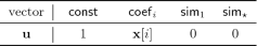
It returns \(\mathsf {ct}=({\mathbf {x},\mathsf {ict}})\) as the ciphertext.
-
\(\mathsf {Dec}({\mathsf {sk},\mathsf {ct}})\) parses \(\mathsf {sk}\) as \(({y,\mathsf {isk}_1,\dots ,\mathsf {isk}_m})\) and \(\mathsf {ct}\) as \(({\mathbf {x},\mathsf {ict}})\), and returns \(\bot \) if \(y(\mathbf {x})=0\). Otherwise, it does the following:
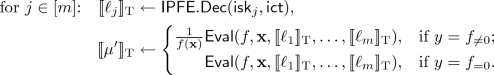
The algorithm returns \( \mathopen [\!\mathopen [{\mu '}\mathclose ]\!\mathclose ] _\text {T}\) as the decapsulated pad. Note: We show the correctness of the scheme. First, by the correctness of IPFE and the definition of vectors \(\mathbf{v}_j, \mathbf{u}\), we have \(\ell _j=\langle {\mathbf {u},\mathbf {v}_j}\rangle =L_j(\mathbf {x})\) for all \(j\in [m]\). Next, by the linearity of \(\mathsf {Eval}\) in \(\ell _1,\dots ,\ell _m\), we can evaluate the garbling in the exponent of the target group and obtain \(\mathsf {Eval}({f,\mathbf {x},\ell _1,\dots ,\ell _m}) = \alpha f(\mathbf{x}) + \beta \) in the exponent. In the two cases where decapsulation should succeed, we have
$$\begin{aligned} \alpha f(\mathbf {x})+\beta ={\left\{ \begin{array}{ll} \mu f(\mathbf {x}),&{} \text {if }y=f_{\ne 0}\text { and }f(\mathbf {x})\ne 0;\\ \mu ,&{} \text {if }y=f_{=0}\text { and }f(\mathbf {x})=0. \end{array}\right. } \end{aligned}$$In both cases, the \(\mu '\) above equals to \(\mu \). Therefore, \(\mathsf {Dec}\) correctly decapsulates the pad.
 for the index set
  . The algorithm returns
  and garbles the function f underlying y as follows:
 for the following vector
 encrypting the vector

Theorem 14
Suppose in Construction 13, the AKGS is piecewise secure and the IPFE scheme is function-hiding, then the constructed 1-ABE scheme is 1-key 1-ciphertext secure.
We refer the readers to the full version for the formal proof.
Notes
- 1.
Some works call x a set of attributes, and each bit or component of x an attribute. We treat the attribute as a single vector.
- 2.
More precisely, they construct ABE for read-once branching programs. For general branching programs, one can duplicate each component in the attribute for the number of times it is accessed [43]. As such, the ciphertext size grows linearly with the size of the branching program.
- 3.
An ABP is specified by a directed graph, with edges weighted by affine functions of the input. The size of an ABP is measured by the number of vertices (instead of edges) in the graph.
- 4.
Message-hiding encodings [42] are a weaker variant of randomized encodings that allow encoding a public computation f, x with a secret message m such that the encoding reveals m if and only if \(f(x)=1\). Such encodings are succinct if the time to encode is much smaller than the running time of the computation. A pair of ABE secret key for predicate f and ciphertext for attribute x and message m is a message-hiding encoding.
- 5.
DFA and NFA both characterize regular languages, yet a DFA recognizing a language could have exponentially more states than an NFA recognizing the same language. In this work, by ABE for DFA/NFA, we mean ABE schemes that run in time polynomial in the description size of the finite automata.
- 6.
As mentioned in Footnote 2, read-once restriction can be circumvented by duplicating attribute components at the cost of losing ciphertext compactness.
- 7.
- 8.
We can also handle policies of the form \(f_{=0}\) so that \(\mu \) is revealed if and only if \(f(\mathbf{x}) = 0\). For simplicity, we focus on one case in this overview.
- 9.
For simplicity, in this overview, we assume there is only one accepting state.
- 10.
This means \(\mathsf {RevSamp}\) is deterministic, and we can reversely sample \(\ell _\text {init}\) in the exponent and when the randomness is not uniform, which is important for our construction.
- 11.
Our scheme readily extends to be based on k-Lin. However, that makes the scheme more complex to present. We choose to present this scheme using SXDH in this paper.
- 12.
The views expressed are those of the authors and do not reflect the official policy or position of the Department of Defense, the National Science Foundation, or the U.S. Government.
References
Agrawal, S., Chase, M.: Simplifying design and analysis of complex predicate encryption schemes. In: Coron, J.-S., Nielsen, J.B. (eds.) EUROCRYPT 2017, Part I. LNCS, vol. 10210, pp. 627–656. Springer, Cham (2017). https://doi.org/10.1007/978-3-319-56620-7_22
Agrawal, S., Libert, B., Stehlé, D.: Fully secure functional encryption for inner products, from standard assumptions. In: Robshaw, M., Katz, J. (eds.) CRYPTO 2016, Part III. LNCS, vol. 9816, pp. 333–362. Springer, Heidelberg (2016). https://doi.org/10.1007/978-3-662-53015-3_12
Agrawal, S., Maitra, M.: FE and iO for turing machines from minimal assumptions. In: Beimel, A., Dziembowski, S. (eds.) TCC 2018, Part II. LNCS, vol. 11240, pp. 473–512. Springer, Cham (2018). https://doi.org/10.1007/978-3-030-03810-6_18
Agrawal, S., Maitra, M., Yamada, S.: Attribute based encryption (and more) for nondeterministic finite automata from LWE. In: Boldyreva, A., Micciancio, D. (eds.) CRYPTO 2019, Part II. LNCS, vol. 11693, pp. 765–797. Springer, Cham (2019). https://doi.org/10.1007/978-3-030-26951-7_26
Agrawal, S., Maitra, M., Yamada, S.: Attribute based encryption for deterministic finite automata from \(\sf DLIN\). In: Hofheinz, D., Rosen, A. (eds.) TCC 2019, Part II. LNCS, vol. 11892, pp. 91–117. Springer, Cham (2019). https://doi.org/10.1007/978-3-030-36033-7_4
Ananth, P., Chen, Y.-C., Chung, K.-M., Lin, H., Lin, W.-K.: Delegating RAM computations with adaptive soundness and privacy. In: Hirt, M., Smith, A. (eds.) TCC 2016, Part II. LNCS, vol. 9986, pp. 3–30. Springer, Heidelberg (2016). https://doi.org/10.1007/978-3-662-53644-5_1
Ananth, P., Fan, X., Shi, E.: Towards attribute-based encryption for RAMs from LWE: sub-linear decryption, and more. Cryptology ePrint Archive, Report 2018/273 (2018). https://eprint.iacr.org/2018/273
Ananth, P., Sahai, A.: Projective arithmetic functional encryption and indistinguishability obfuscation from degree-5 multilinear maps. In: Coron, J.-S., Nielsen, J.B. (eds.) EUROCRYPT 2017, Part I. LNCS, vol. 10210, pp. 152–181. Springer, Cham (2017). https://doi.org/10.1007/978-3-319-56620-7_6
Ananth, P.V., Sahai, A.: Functional encryption for turing machines. In: Kushilevitz, E., Malkin, T. (eds.) TCC 2016, Part I. LNCS, vol. 9562, pp. 125–153. Springer, Heidelberg (2016). https://doi.org/10.1007/978-3-662-49096-9_6
Applebaum, B., Ishai, Y., Kushilevitz, E.: Cryptography in NC\(^0\). In: 45th FOCS, pp. 166–175. IEEE Computer Society Press, October 2004
Applebaum, B., Ishai, Y., Kushilevitz, E.: How to garble arithmetic circuits. In: Ostrovsky, R. (ed.) 52nd FOCS, pp. 120–129. IEEE Computer Society Press, October 2011
Attrapadung, N.: Dual system encryption via doubly selective security: framework, fully secure functional encryption for regular languages, and more. In: Nguyen, P.Q., Oswald, E. (eds.) EUROCRYPT 2014. LNCS, vol. 8441, pp. 557–577. Springer, Heidelberg (2014). https://doi.org/10.1007/978-3-642-55220-5_31
Attrapadung, N.: Dual system encryption framework in prime-order groups via computational pair encodings. In: Cheon, J.H., Takagi, T. (eds.) ASIACRYPT 2016, Part II. LNCS, vol. 10032, pp. 591–623. Springer, Heidelberg (2016). https://doi.org/10.1007/978-3-662-53890-6_20
Attrapadung, N.: Dual system framework in multilinear settings and applications to fully secure (compact) ABE for unbounded-size circuits. In: Fehr, S. (ed.) PKC 2017, Part II. LNCS, vol. 10175, pp. 3–35. Springer, Heidelberg (2017). https://doi.org/10.1007/978-3-662-54388-7_1
Beimel, A., Gal, A.: On arithmetic branching programs. In: Proceedings of the 13th Annual IEEE Conference on Computational Complexity, pp. 68–80 (1998)
Bethencourt, J., Sahai, A., Waters, B.: Ciphertext-policy attribute-based encryption. In: 2007 IEEE Symposium on Security and Privacy (SP 2007), pp. 321–334, May 2007
Bishop, A., Jain, A., Kowalczyk, L.: Function-hiding inner product encryption. In: Iwata, T., Cheon, J.H. (eds.) ASIACRYPT 2015, Part I. LNCS, vol. 9452, pp. 470–491. Springer, Heidelberg (2015). https://doi.org/10.1007/978-3-662-48797-6_20
Bitansky, N., Garg, S., Lin, H., Pass, R., Telang, S.: Succinct randomized encodings and their applications. In: Servedio, R.A., Rubinfeld, R. (eds.) 47th ACM STOC, pp. 439–448. ACM Press, June 2015
Boneh, D., et al.: Fully key-homomorphic encryption, arithmetic circuit ABE and compact garbled circuits. In: Nguyen, P.Q., Oswald, E. (eds.) EUROCRYPT 2014. LNCS, vol. 8441, pp. 533–556. Springer, Heidelberg (2014). https://doi.org/10.1007/978-3-642-55220-5_30
Boyen, X., Li, Q.: Attribute-based encryption for finite automata from LWE. In: Au, M.-H., Miyaji, A. (eds.) ProvSec 2015. LNCS, vol. 9451, pp. 247–267. Springer, Cham (2015). https://doi.org/10.1007/978-3-319-26059-4_14
Canetti, R., Holmgren, J., Jain, A., Vaikuntanathan, V.: Succinct garbling and indistinguishability obfuscation for RAM programs. In: Servedio, R.A., Rubinfeld, R. (eds.) 47th ACM STOC, pp. 429–437. ACM Press, June 2015
Chen, J., Gay, R., Wee, H.: Improved dual system ABE in prime-order groups via predicate encodings. In: Oswald, E., Fischlin, M. (eds.) EUROCRYPT 2015, Part II. LNCS, vol. 9057, pp. 595–624. Springer, Heidelberg (2015). https://doi.org/10.1007/978-3-662-46803-6_20
Chen, J., Gong, J., Kowalczyk, L., Wee, H.: Unbounded ABE via bilinear entropy expansion, revisited. In: Nielsen, J.B., Rijmen, V. (eds.) EUROCRYPT 2018, Part I. LNCS, vol. 10820, pp. 503–534. Springer, Cham (2018). https://doi.org/10.1007/978-3-319-78381-9_19
Chen, J., Gong, J., Wee, H.: Improved inner-product encryption with adaptive security and full attribute-hiding. In: Peyrin, T., Galbraith, S. (eds.) ASIACRYPT 2018, Part II. LNCS, vol. 11273, pp. 673–702. Springer, Cham (2018). https://doi.org/10.1007/978-3-030-03329-3_23
Datta, P., Dutta, R., Mukhopadhyay, S.: Functional encryption for inner product with full function privacy. In: Cheng, C.-M., Chung, K.-M., Persiano, G., Yang, B.-Y. (eds.) PKC 2016, Part I. LNCS, vol. 9614, pp. 164–195. Springer, Heidelberg (2016). https://doi.org/10.1007/978-3-662-49384-7_7
Escala, A., Herold, G., Kiltz, E., Ràfols, C., Villar, J.: An algebraic framework for Diffie-Hellman assumptions. In: Canetti, R., Garay, J.A. (eds.) CRYPTO 2013, Part II. LNCS, vol. 8043, pp. 129–147. Springer, Heidelberg (2013). https://doi.org/10.1007/978-3-642-40084-1_8
Goldwasser, S., Kalai, Y.T., Popa, R.A., Vaikuntanathan, V., Zeldovich, N.: How to run turing machines on encrypted data. In: Canetti, R., Garay, J.A. (eds.) CRYPTO 2013, Part II. LNCS, vol. 8043, pp. 536–553. Springer, Heidelberg (2013). https://doi.org/10.1007/978-3-642-40084-1_30
Goldwasser, S., Kalai, Y.T., Popa, R.A., Vaikuntanathan, V., Zeldovich, N.: Reusable garbled circuits and succinct functional encryption. In: Boneh, D., Roughgarden, T., Feigenbaum, J. (eds.) 45th ACM STOC, pp. 555–564. ACM Press, June 2013
Gong, J., Waters, B., Wee, H.: ABE for DFA from k-Lin. In: Boldyreva, A., Micciancio, D. (eds.) CRYPTO 2019, Part II. LNCS, vol. 11693, pp. 732–764. Springer, Cham (2019). https://doi.org/10.1007/978-3-030-26951-7_25
Gorbunov, S., Vaikuntanathan, V., Wee, H.: Attribute-based encryption for circuits. In: Boneh, D., Roughgarden, T., Feigenbaum, J. (eds.) 45th ACM STOC, pp. 545–554. ACM Press, June 2013
Gorbunov, S., Vinayagamurthy, D.: Riding on asymmetry: efficient ABE for branching programs. In: Iwata, T., Cheon, J.H. (eds.) ASIACRYPT 2015, Part I. LNCS, vol. 9452, pp. 550–574. Springer, Heidelberg (2015). https://doi.org/10.1007/978-3-662-48797-6_23
Goyal, V., Pandey, O., Sahai, A., Waters, B.: Attribute-based encryption for fine-grained access control of encrypted data. In: Juels, A., Wright, R.N., di Vimercati, S.C. (eds.) ACM CCS 2006, pp. 89–98. ACM Press, October/November 2006. Available as Cryptology ePrint Archive Report 2006/309
Hofheinz, D., Koch, J., Striecks, C.: Identity-based encryption with (almost) tight security in the multi-instance, multi-ciphertext setting. In: Katz, J. (ed.) PKC 2015. LNCS, vol. 9020, pp. 799–822. Springer, Heidelberg (2015). https://doi.org/10.1007/978-3-662-46447-2_36
Ishai, Y., Kushilevitz, E.: Private simultaneous messages protocols with applications. In: Proceedings of the 5th ISTCS, pp. 174–183 (1997)
Ishai, Y., Kushilevitz, E.: Randomizing polynomials: a new representation with applications to round-efficient secure computation. In: 41st FOCS, pp. 294–304. IEEE Computer Society Press, November 2000
Ishai, Y., Kushilevitz, E.: Perfect constant-round secure computation via perfect randomizing polynomials. In: Widmayer, P., Ruiz, F.T., Bueno, R.M., Hennessy, M., Eidenbenz, S., Conejo, R. (eds.) ICALP 2002. LNCS, vol. 2380, pp. 244–256. Springer, Heidelberg (2002). https://doi.org/10.1007/3-540-45465-9_22
Ishai, Y., Wee, H.: Partial garbling schemes and their applications. In: Esparza, J., Fraigniaud, P., Husfeldt, T., Koutsoupias, E. (eds.) ICALP 2014, Part I. LNCS, vol. 8572, pp. 650–662. Springer, Heidelberg (2014). https://doi.org/10.1007/978-3-662-43948-7_54
Jafargholi, Z., Kamath, C., Klein, K., Komargodski, I., Pietrzak, K., Wichs, D.: Be adaptive, avoid overcommitting. In: Katz, J., Shacham, H. (eds.) CRYPTO 2017, Part I. LNCS, vol. 10401, pp. 133–163. Springer, Cham (2017). https://doi.org/10.1007/978-3-319-63688-7_5
Katz, J., Sahai, A., Waters, B.: Predicate encryption supporting disjunctions, polynomial equations, and inner products. J. Cryptol. 26(2), 191–224 (2013)
Kim, S., Lewi, K., Mandal, A., Montgomery, H., Roy, A., Wu, D.J.: Function-hiding inner product encryption is practical. In: Catalano, D., De Prisco, R. (eds.) SCN 2018. LNCS, vol. 11035, pp. 544–562. Springer, Cham (2018). https://doi.org/10.1007/978-3-319-98113-0_29
Kitagawa, F., Nishimaki, R., Tanaka, K., Yamakawa, T.: Adaptively secure and succinct functional encryption: improving security and efficiency, simultaneously. In: Boldyreva, A., Micciancio, D. (eds.) CRYPTO 2019, Part III. LNCS, vol. 11694, pp. 521–551. Springer, Cham (2019). https://doi.org/10.1007/978-3-030-26954-8_17
Koppula, V., Lewko, A.B., Waters, B.: Indistinguishability obfuscation for turing machines with unbounded memory. In: Servedio, R.A., Rubinfeld, R. (eds.) 47th ACM STOC, pp. 419–428. ACM Press, June 2015
Kowalczyk, L., Liu, J., Malkin, T., Meiyappan, K.: Mitigating the one-use restriction in attribute-based encryption. In: Lee, K. (ed.) ICISC 2018. LNCS, vol. 11396, pp. 23–36. Springer, Cham (2019). https://doi.org/10.1007/978-3-030-12146-4_2
Kowalczyk, L., Wee, H.: Compact adaptively secure ABE for \(\sf NC^1\) from k-Lin. In: Ishai, Y., Rijmen, V. (eds.) EUROCRYPT 2019, Part I. LNCS, vol. 11476, pp. 3–33. Springer, Cham (2019). https://doi.org/10.1007/978-3-030-17653-2_1
Lewko, A., Okamoto, T., Sahai, A., Takashima, K., Waters, B.: Fully secure functional encryption: attribute-based encryption and (hierarchical) inner product encryption. In: Gilbert, H. (ed.) EUROCRYPT 2010. LNCS, vol. 6110, pp. 62–91. Springer, Heidelberg (2010). https://doi.org/10.1007/978-3-642-13190-5_4
Lewko, A.B., Waters, B.: New techniques for dual system encryption and fully secure HIBE with short ciphertexts. In: Micciancio, D. (ed.) TCC 2010. LNCS, vol. 5978, pp. 455–479. Springer, Heidelberg (2010). https://doi.org/10.1007/978-3-642-11799-2_27
Lewko, A., Waters, B.: Unbounded HIBE and attribute-based encryption. In: Paterson, K.G. (ed.) EUROCRYPT 2011. LNCS, vol. 6632, pp. 547–567. Springer, Heidelberg (2011). https://doi.org/10.1007/978-3-642-20465-4_30
Lewko, A., Waters, B.: New proof methods for attribute-based encryption: achieving full security through selective techniques. In: Safavi-Naini, R., Canetti, R. (eds.) CRYPTO 2012. LNCS, vol. 7417, pp. 180–198. Springer, Heidelberg (2012). https://doi.org/10.1007/978-3-642-32009-5_12
Lin, H.: Indistinguishability obfuscation from SXDH on 5-linear maps and locality-5 PRGs. In: Katz, J., Shacham, H. (eds.) CRYPTO 2017, Part I. LNCS, vol. 10401, pp. 599–629. Springer, Cham (2017). https://doi.org/10.1007/978-3-319-63688-7_20
Lin, H., Vaikuntanathan, V.: Indistinguishability obfuscation from DDH-like assumptions on constant-degree graded encodings. In: Dinur, I. (ed.) 57th FOCS, pp. 11–20. IEEE Computer Society Press, October 2016
Nisan, N.: Lower bounds for non-commutative computation (extended abstract). In: 23rd ACM STOC, pp. 410–418. ACM Press, May 1991
Okamoto, T., Takashima, K.: Hierarchical predicate encryption for inner-products. In: Matsui, M. (ed.) ASIACRYPT 2009. LNCS, vol. 5912, pp. 214–231. Springer, Heidelberg (2009). https://doi.org/10.1007/978-3-642-10366-7_13
Okamoto, T., Takashima, K.: Fully secure functional encryption with general relations from the decisional linear assumption. In: Rabin, T. (ed.) CRYPTO 2010. LNCS, vol. 6223, pp. 191–208. Springer, Heidelberg (2010). https://doi.org/10.1007/978-3-642-14623-7_11
Okamoto, T., Takashima, K.: Fully secure unbounded inner-product and attribute-based encryption. In: Wang, X., Sako, K. (eds.) ASIACRYPT 2012. LNCS, vol. 7658, pp. 349–366. Springer, Heidelberg (2012). https://doi.org/10.1007/978-3-642-34961-4_22
Shen, E., Shi, E., Waters, B.: Predicate privacy in encryption systems. In: Reingold, O. (ed.) TCC 2009. LNCS, vol. 5444, pp. 457–473. Springer, Heidelberg (2009). https://doi.org/10.1007/978-3-642-00457-5_27
Tomida, J., Abe, M., Okamoto, T.: Efficient functional encryption for inner-product values with full-hiding security. In: Bishop, M., Nascimento, A.C.A. (eds.) ISC 2016. LNCS, vol. 9866, pp. 408–425. Springer, Cham (2016). https://doi.org/10.1007/978-3-319-45871-7_24
Waters, B.: Dual system encryption: realizing fully secure IBE and HIBE under simple assumptions. In: Halevi, S. (ed.) CRYPTO 2009. LNCS, vol. 5677, pp. 619–636. Springer, Heidelberg (2009). https://doi.org/10.1007/978-3-642-03356-8_36
Waters, B.: Functional encryption for regular languages. In: Safavi-Naini, R., Canetti, R. (eds.) CRYPTO 2012. LNCS, vol. 7417, pp. 218–235. Springer, Heidelberg (2012). https://doi.org/10.1007/978-3-642-32009-5_14
Wee, H.: Dual system encryption via predicate encodings. In: Lindell, Y. (ed.) TCC 2014. LNCS, vol. 8349, pp. 616–637. Springer, Heidelberg (2014). https://doi.org/10.1007/978-3-642-54242-8_26
Wee, H.: Attribute-hiding predicate encryption in bilinear groups, revisited. In: Kalai, Y., Reyzin, L. (eds.) TCC 2017, Part I. LNCS, vol. 10677, pp. 206–233. Springer, Cham (2017). https://doi.org/10.1007/978-3-319-70500-2_8
Yao, A.C.-C.: How to generate and exchange secrets (extended abstract). In: 27th FOCS, pp. 162–167. IEEE Computer Society Press, October 1986
Acknowledgments
The authors were supported by NSF grantsFootnote 12 CNS-1528178, CNS-1929901, CNS-1936825 (CAREER). The authors thank Hoeteck Wee for helpful discussions and the anonymous reviewers for insightful comments.
Author information
Authors and Affiliations
Corresponding authors
Editor information
Editors and Affiliations
Rights and permissions
Copyright information
© 2020 International Association for Cryptologic Research
About this paper

Cite this paper
Lin, H., Luo, J. (2020). Compact Adaptively Secure ABE from k-Lin: Beyond \(\mathsf {NC}^1\) and Towards \(\mathsf {NL}\). In: Canteaut, A., Ishai, Y. (eds) Advances in Cryptology – EUROCRYPT 2020. EUROCRYPT 2020. Lecture Notes in Computer Science(), vol 12107. Springer, Cham. https://doi.org/10.1007/978-3-030-45727-3_9
Download citation
DOI: https://doi.org/10.1007/978-3-030-45727-3_9
Published:
Publisher Name: Springer, Cham
Print ISBN: 978-3-030-45726-6
Online ISBN: 978-3-030-45727-3
eBook Packages: Computer ScienceComputer Science (R0)
