Quantum Collision Attacks on AES-Like Hashing with Low Quantum Random Access Memories

Abstract

At EUROCRYPT 2020, Hosoyamada and Sasaki proposed the first dedicated quantum attack on hash functions—a quantum version of the rebound attack exploiting differentials whose probabilities are too low to be useful in the classical setting. This work opens up a new perspective toward the security of hash functions against quantum attacks. In particular, it tells us that the search for differentials should not stop at the classical birthday bound. Despite these interesting and promising implications, the concrete attacks described by Hosoyamada and Sasaki make use of large quantum random access memories (qRAMs), a resource whose availability in the foreseeable future is controversial even in the quantum computation community. Without large qRAMs, these attacks incur significant increases in time complexities. In this work, we reduce or even avoid the use of qRAMs by performing a quantum rebound attack based on differentials with non-full-active super S-boxes. Along the way, an MILP-based method is proposed to systematically explore the search space of useful truncated differentials with respect to rebound attacks. As a result, we obtain improved attacks on AES-MMO, AES-MP, and the first classical collision attacks on 4- and 5-round Grøstl-512. Interestingly, the use of non-full-active super S-box differentials in the analysis of AES-MMO gives rise to new difficulties in collecting enough starting points. To overcome this issue, we consider attacks involving two message blocks to gain more degrees of freedom, and we successfully compress the qRAM demand of the collision attacks on AES-MMO and AES-MP (EUROCRYPT 2020) from $2^{48}$ to a range from $2^{16}$ to 0, while still maintaining a comparable time complexity. To the best of our knowledge, these are the first dedicated quantum attacks on hash functions that slightly outperform Chailloux, Naya-Plasencia, and Schrottenloher’s generic quantum collision attack (ASIACRYPT 2017) in a model where large qRAMs are not available. This work demonstrates again how a clever combination of classical cryptanalytic technique and quantum computation leads to improved attacks, and shows that the direction pointed out by Hosoyamada and Sasaki deserves further investigation.

1 Introduction

Shor’s seminal work  [44] showed that a sufficiently large quantum computer allows to factor numbers and compute discrete logarithms in polynomial time, which can be devastating to many public-key schemes in use today. To prepare for the future, the public-key cryptography community and standardization bodies have put substantial effort in the research of post-quantum public-key cryptography. In particular, NIST has initiated a process to solicit, evaluate, and standardize one or more quantum-resistant public-key cryptographic algorithms  [41]. In contrast, the research on how quantum computation would change the landscape of the security of symmetric-key cryptography seems to be less active. For almost twenty years, it was generally believed that the quadratic speedup in an exhaustive search attack due to Grover’s algorithm  [16] is the only advantage an attacker equipped with a quantum computer would have when attacking symmetric-key ciphers, and thus doubling the key length addresses the concern.

This naive view started to change with the initial work of Kuwakado and Morii, who showed that the classically provable secure Even-Mansour cipher and the three-round Feistel network can be broken in polynomial time with the help of a quantum computer  [28, 29]. Several years later, more generic constructions were broken  [25, 32]. Almost all these attacks enjoying exponential speedups rely on Simon’s algorithm  [45] to find a key-dependent hidden period, where accesses to the quantum superposition oracle of the keyed primitives are necessary. This is a quite strong requirement, and sometimes its practical relevance is questioned. Therefore, attacks with higher complexities are still meaningful if they do not need to make online queries to superposition oracles of keyed primitives  [2, 18].

When we apply quantum algorithms to keyless primitives, online queries are not needed since all computations are public and can be done offline. Classical algorithms find collisions of an n-bit ideal hash function with time complexity $O(2^{n/2})$. In the quantum setting, BHT algorithm  [6] finds collisions with a query complexity of $O(2^{n/3})$ if an $O(2^{n/3})$-qubit quantum random access memory (qRAM) is available  [6]. However, it is generally admitted that the difficulty of fabricating large qRAMs is enormous  [13, 14], and thus quantum algorithms (even with relatively higher time complexities) using less or no qRAMs are preferable. Chailloux, Naya-Plasencia, and Schrottenloher first overcome the $O(2^{n/2})$ classical bound without using large qRAMs  [7]. This algorithm has a time complexity of $O(2^{2n/5})$, with quantum memory of O(n) and a classical memory of $O(2^{n/5})$. Also, quantum algorithms for the generalized birthday problem (or the k-XOR problem) in settings with or without large qRAMs can be found in  [15, 39].

The above mentioned attacks on hash functions are generic in the sense that they do not exploit any internal characteristics of the targets. In fact, before year 2020, no dedicated quantum attack is seen in the open literature, in stark contrast to the line of cryptanalytic research targeting keyed primitives in the quantum setting, where attempts to escalate dedicated attacks are plentiful (e.g., differential and linear attacks  [26], impossible differential attacks  [47], meet-in-the-middle attacks  [4, 19], slide attacks  [3, 10], etc.). The first dedicated quantum attack on hash functions was presented at EUROCRYPT 2020 by Hosoyamada and Sasaki  [20], showing that differentials whose probability is too low to be useful in the classical setting may be exploited in quantum attacks. They applied a quantum version of the rebound attack on AES-MMO and Whirlpool, and gave the first quantum collision attack on AES-MMO.

Our Contribution. Motivated by the fact that the availability of large qRAMs is controversial  [1, 13, 14], we try to lower the qRAM requirements of Hosoyamada and Sasaki’s attacks  [20]. With the application of non-full-active super S-box techniques  [42], we can significantly reduce (or even avoid) the use of qRAMs. Along the way, we propose an MILP-based method to systematically explore the search space of useful differential trails with respect to rebound attacks, which is of independent interest. With the help of this method, we find differentials leading to improved attacks in both the classical and quantum settings. For example, we present the first classical collision attacks on 4-round and 5-round Grøstl-512, where the complexity of the 4-round attack is significantly better than previously known best attacks on 3-round Grøstl-512. Also, we obtain improved semi-free-start collision attacks on Grøstl-256.

Table 1. Classical and quantum collision attacks on AES-MMO, AES-MP, Grøstl. Q-Model I and II are quantum settings with qRAM and without qRAM, respectively.

In the analysis of AES-MMO and AES-MP, the differentials we find leading to non-full-active super S-boxes for the inbound phase cannot generate enough starting points to produce a collision due to the probabilistic nature of the outbound phase of the attack. To overcome this difficulty, we consider two blocks of messages, execute rebound attacks on the second message block, and borrow degrees of freedom from the first one. As a result, we successfully compress the qRAM demand from $2^{48}$ to a range from $2^{16}$ to 0, while still maintaining a comparable time complexity. Hosoyamada and Sasaki’s work  [20] tells us that certain worthless truncated differential trails in the classical setting are exploitable in the quantum setting. Our work further enlarges the space of quantumly exploitable truncated differential trails by considering collisions produced by two-block messages, where trails unable to generate enough starting points during the inbound phase of a single-block rebound collision attack are included. We believe this observation will inspire new attacks on hash functions in the quantum setting. Moreover, in a model without large qRAMs, Hosoyamada and Sasaki’s attacks are inferior to the generic attack by Chailloux, Naya-Plasencia, and Schrottenloher  [7]:

“However, in the setting that a small quantum computer of polynomial size and exponential large classical memory is available, our rebound attack is lower than the best attack by Chailloux et al. (see  [20, Sect. 1.1, Page 6])”

To the best of our knowledge, our work is the first dedicated quantum attack on hash functions that slightly surpasses the generic quantum collision attack  [7] in a model where large qRAMs are not available. In the quantum time-space scenario, our attacks also gain improvements. For example, the attack without qRAM on 7-round AES-MMO needs a time complexity of $2^{45.8}$. If we have S quantum computers in parallel, we will find the collision with time $2^{45.8}/\sqrt{S}$. In the same setting, Hosoyamada and Sasaki  [20]’s attack needs about $2^{59.5}/\sqrt{S}$ time complexity. A summary of our attacks on AES-MMO, AES-MP, and Grøstl is given in Table 1.

Organization. Section 2 gives a brief introduction of AES-like hashing, quantum computation, and qRAMs. We describe the classical technique for collision attacks on hash functions with the rebound technique, and show how to search for useful truncated differential trails with non-full-active super S-boxes by MILP with multiple objectives in Sect. 3. This is followed by Sect. 4, to Sect. 7, which present our improved attacks on AES-MMO, AES-MP, and Grøstl. Section 8 concludes the paper.

2 Preliminaries

In this section, we give a brief introduction of AES-like hashing and quantum computation, and familiarize the readers with the functionalities of quantum random access memories (qRAMs).

2.1 AES-Like Hashing

To be concrete, we first recall the round function of AES-128  [8]. It operates on a 16-byte state arranged into a rectangular shape and contains four major transformations as illustrated in Fig. 1: SubBytes (SB), ShiftRows (SR), MixColumns (MC), and AddRoundKey (AK). The parameters like the numbers of rows and columns, the sizes of the cells, the order of the transformations, and the roles played by the rows and columns can be altered by making compatible changes to the operations involved to produce new designs, which are loosely called as AES-like round functions. In this paper, we assume the MixColumns is to multiply an MDS matrix to each column of the state.

Fig. 1.

The round function of AES

By using (keyed) permutations with AES-like round functions in certain hashing modes, compression functions (denoted as CF) can be constructed. For example, the MD, MMO, and MP hashing modes  [35, Section 9.4] are illustrated in Fig. 2. Plugging such compression functions into the Merkle-Damgård construction  [9, 36], one arrives at AES-like hashings. Concrete designs include AES-MMO, AES-MP, and Grøstl  [11], which are the main targets of this work.

Fig. 2.

Common Hashing Modes

2.2 Quantum Computation and Quantum RAM

The states of an n-qubit quantum system can be described as unit vectors in $\mathbb {C}^{2^n}$ under the orthonormal basis , alternatively written as . Quantum algorithms are typically realized by manipulating the state of an n-qubit system through a series of unitary transformations and measurements, where all unitary transformations can be implemented as a sequence of single-qubit and two-qubit transformations, which are called quantum gates in the standard quantum circuit model  [40]. The efficiency of a quantum algorithm is quantified in terms of the amount of quantum gates used.

Superposition Oracles for Classical Circuit. Given a Boolean function $f: \mathbb {F}_2^n \rightarrow \mathbb {F}_2$. The superposition oracle of f is the unitary transformation $\mathcal {U}_f$ acting on an $(n+1)$-qubit system sending a standard basis vector to , where $x \in \mathbb {F}_2^n$ and $y \in \mathbb {F}_2$. As a linear operator, $\mathcal {U}_f$ acts on superposition states as

(1)

Note that $\mathcal {U}_f$ can be implemented efficiently in the quantum circuit model as long as there is an efficient classical circuit that computes f. To build the quantum circuit of $\mathcal {U}_f$, we first construct an efficient reversible circuit of f and substitute quantum gates for each of the reversible gates involved.

Grover’s Algorithm. Given a search space of $2^n$ elements, say $\{ x : x \in \mathbb {F}_2^n \}$, and a Boolean function or predicate $f: \mathbb {F}_2^n \rightarrow \mathbb {F}_2$, the best classical algorithm with a black-box access to f requires about $2^{n}$ evaluations of the black-box oracle to identify x such that $f(x) = 1$ with probability one (For the sake of simplicity, we assume that there is only one such x). In the quantum setting, Grover’s algorithm solves the same problem with about $O(\sqrt{2^n})$ calls to a quantum oracle $\mathcal {U}_f$ that outputs upon input of . Starting with a uniform superposition

by applying the Hadamard transformation $H^{\otimes n}$ to . Then Grover’s algorithm iteratively apply the unitary transformation to such that the amplitudes of those values x with $f(x) = 1$ are amplified. Then a final measurement gives a value x of interest with an overwhelming probability  [16].

One caveat here: complexity can be hidden in the complexity of constructing the oracle circuit employed by Grover’s algorithm. The speedup of the search would be illusory unless the oracle circuit can be implemented efficiently. Therefore, it is important to have a clear view on what resources it takes to implement the oracle. For example, a large qRAM is necessary if it requires a large qRAM to implement the oracle efficiently.

Quantum Amplitude Amplification. Let be a projector with , and $\mathcal {A}$ be a unitary operator such that , where and . Then there exists a quantum algorithm that requires exclusively $\lfloor \frac{\pi }{4\theta } - \frac{1}{2} \rfloor$ calls to $\mathcal {U}_{\mathcal {P}}$, $\mathcal {U}_P^\dagger$, $\mathcal {A}$, and $\mathcal {A}^\dagger$, after a final measurement, to produce a quantum state close to , where $\sin (\theta ) = |\alpha |$, and the effect of the unitary operator $\mathcal {U}_{\mathcal {P}}$ on base vectors satisfying and otherwise  [5].

The quantum amplitude amplification can be regarded as a generalization of Grover’s algorithm in which $\mathcal {A}$ is restricted to produce an equal superposition of all basis vectors. Similarly, when analyzing the complexity of the quantum amplitude amplification, we should take into account the complexities for implementing $\mathcal {U}_{\mathcal {P}}$ and $\mathcal {A}$.

Quantum Random Access Memories (qRAM). A quantum random access memory (qRAM) is a quantum analogue of a classical random access memory (RAM), which uses n-qubit to address any quantum superposition of $2^n$ memory cells. Given a list of classical data $L = \{ x_0, \cdots , x_{2^n-1} \}$ with $x_i \in \mathbb {F}_2^m$, the qRAM for L is modeled as an unitary transformation $\mathcal {U}_{\mathsf {qRAM}}^L$ such that

(2)

where $i \in \mathbb {F}_2^n$, $y \in \mathbb {F}_2^m$, and and may be regarded as the address and output registers respectively. Therefore, we can access any quantum superposition of the data cells by using the corresponding superposition of addresses:

(3)

For the time being, it is unknown how a working qRAM (at least for large qRAMs) can be built. Nevertheless, this disappointing fact does not stop researchers from working in a model where large qRAMs are available, in the same spirit that people started to work on classical and quantum algorithms long before a classical or quantum computer had been built. From another perspective, the absence of large qRAMs and the fact that a qRAM of size O(n) can be simulated with a quantum circuit of size O(n) makes it quite meaningful to conduct research in an attempt to reduce or even avoid the use of qRAM in quantum algorithms.

3 MILP Models for the Rebound Attack

For the sake of concreteness, we restrict our discussion to collision attacks on AES-MMO, which is standardized by Zigbee and used by many multi-party computation protocols  [17, 27] due to its efficiency. Assume that there is a differential trail for $E_K$ with probability p whose input and output differences share a common value $\varDelta$. Given around 1/p pairs of input messages with difference $\varDelta$, we expect one pair $(m, m \oplus \varDelta )$ follows this differential trail: $E_K(m) \oplus E_K(m \oplus \varDelta ) = \varDelta$. If this is the case, the differences of the outputs of the MMO construction is

$$\begin{aligned} ( m \oplus E_K(m)) \oplus (m \oplus \varDelta \oplus E_K(m \oplus \varDelta )) = \varDelta \oplus \varDelta = 0, \end{aligned}$$

(4)

that is, a collision. Since K is known in hash functions, it is possible to generate many data pairs which confirm to one particular segment (typically the most difficult part) of the desired trail. Then these pairs are tested to find one fulfilling the remaining part of the trail. This is the basic strategy employed by the so-called rebound attack proposed by Mendel, Rechberger, Schläffer and Thomsen  [31, 33].

In a rebound attack, the target primitive and thus the differential trail covering it is split into three parts. An inbound part is placed at the middle surrounded by two outbound parts. By utilizing the degrees of freedom of the inbound part, many data pairs conforming to the differential of the inbound part (named as inbound differential) can be constructed deterministically or with a very high probability. Then these data pairs, named as starting points, are propagated through the outbound parts to find pairs respecting the outbound differential by chance. Among many improvements and extensions of the rebound attacks  [22,23,24, 38], the super S-box technique  [12, 30] and the non-full-active super S-box technique  [42] are most relevant to our work.

3.1 The Full-Active and Non-Full-Active Super S-Box Techniques

In the context of rebound attacks on AES-MMO, the super S-box technique enlarges the inbound part by one more round than previous analysis by identifying four non-interfering $\mathbb {F}_2^{32} \rightarrow \mathbb {F}_2^{32}$ permutations across two consecutive AES rounds and regarding them as four super S-boxes. Initially, when using the super S-box technique for the inbound phase, researchers only considered differentials activating all cells of the super S-boxes, and we refer the reader to Fig. 3 for an example, where one of the four super S-boxes involved in the inbound phase (surround by the dashed line) is highlighted. To generate starting points under this configuration (full-active super S-box) with complexity one on average, one has to store a table $\mathbb {L}_{\varDelta _{in}}$ whose entry $\mathbb {L}_{\varDelta _{in}}[\varDelta _{out}]$ at index $\varDelta _{out}$ contains the pairs respecting the differential $(\varDelta _{in}, \varDelta _{out})$ of the super S-box  [12, 30]. Since the memory of $\mathbb {L}_{\varDelta _{in}}$ is released after the analysis for one particular input difference $\varDelta _{in}$ is done, we only need the memory to store one copy of $\mathbb {L}_{\varDelta _{in}}$.

Fig. 3.

The differential trail used in Hosoyamada and Sasaki’s quantum collision attack on 7-round AES-MMO  [20] with its inbound part and one of the super S-boxes highlighted

In [42], Sasaki, Wang, Sakiyama, and Ohta found that by using differentials with non-full active super S-boxes, the memory complexity of the inbound phase can be significantly reduced. This is because typically data pairs compatible with a given differential with a non-full-active super S-box can be built up progressively by working on 8-bit values. We refer the reader to  [42] for more details. In what follows, we describe how to generate data pairs respecting a given differential with a non-full-active super S-box through a concrete example shown in Fig. 4. This is also a differential we actually used in our improved attacks on AES-MMO.

Fig. 4.

A differential with non-full-active super S-box

First, we precompute the differential distribution table DDT of the small S-box in table $\mathbb {T}$ using Algorithm 1 and load it into random access memories. As shown in Fig. 4, given the truncated differential of the super S-box $\mathtt {SSB} = \mathtt {SB} \circ \mathtt {MC} \circ \mathtt {SB}$, we can generate data pairs conforming to a given differential $(\varDelta A, \varDelta D)$ for SSB by enumerating $(A[0], \beta ) \in \mathbb {F}_2^{11}$ with Algorithm 2. We remember an easy property for MC when understanding Algorithm 2.

Property 1

$\mathtt {MC} \cdot (X[0], X[1], X[2], X[3])^T = (Y[0], Y[1], Y[2], Y[3])^T$ can be used to fully determine the remaining unknowns if any four of X[0], $\cdots$, X[3], Y[0], $\cdots$, Y[3] are known.

Note that in Algorithm 2, there are 3 DDT accesses to determine a combination of (A[2], C[1], C[2]), hence, we have $2\times 2 \times 2=8$ choices. Following the strategy of Hosoyamada and Sasaki’s attack  [20], we introduce an auxiliary 3-bit variable $\beta$ to specify which combination to choose among the 8 choices. The complexity of Algorithm 2 includes $2+2=4$ small S-boxes evaluations (Step 1 and Step 19) and 3 DDT accesses (Step 6–8). Suppose the differential distribution of the S-box is similar to that of the S-box of AES, i.e., 4-uniform. Therefore, it returns a pair when accessing $\mathbb {T}$ with $(\delta _{in},\delta _{out}) \in \mathbb {F}_2^8\times \mathbb {F}_2^8$ with probability of about $\frac{1}{2}$, and returns empty also with probability of about $\frac{1}{2}$. Hence, Step 6–8 of Algorithm 2 act as a filter of $2^{-3}$. In addition, we have a filter of $2^{-8}$ in Step 19. Therefore, by traversing the 11-bit ($A[0],\beta$), it is expected to return ($2^{8}\times 2^{3}\times 2^{-3}\times 2^{-8}$=) 1 pair which conforms the given input-output differences $(\varDelta {A},\varDelta D)$ of SSB. The total complexity is $2^{11}\cdot 4$ S-box evaluations and $2^{11}\cdot 3$ DDT  accesses.

We consider a more general scenario: a column state A with d c-bit cells is mapped to $D = \mathtt {SB} \circ \mathtt {MC} \circ \mathtt {SB} (A)$, where $\mathtt {SB}$ is a parallel application of d $c \times c$ small S-boxes and $\mathtt {MC}: \mathbb {F}_{2^c}^d \rightarrow \mathbb {F}_{2^c}^d$ is a linear transformation with branch number $d+1$. Assume that a differential of the super S-box $\mathtt {SSB} = \mathtt {SB} \circ \mathtt {MC} \circ \mathtt {SB}$ leads to s non-active $c \times c$ S-boxes, and thus we have $2d - s$ small active S-boxes. To generate a pair respecting a given differential $(\varDelta A, \varDelta D)$ for the SSB, we perform the following steps:

• 1. Guess $d-s$ cells of (A, D) (the guessed positions must be selected within the active cells of (A, D)).

• 2. Compute the values of $d-s$ cells of (B, C) from the guessed $d-s$ cells of (A, D). Compute the differences of $d-s$ active cells of $(\varDelta B, \varDelta C)$.

• 3. Combining with the s non-active cells of $(\varDelta B, \varDelta C)$, we get $(d-s)+s=d$ cells with known differences among the input-output differences of $\mathtt {MC}$. By Property 1, we know all the differences in the truncated differential.

• 4. Since $d-s$ cells of (B, C) have been determined, we need an additional s cells to determine all other cells of (B, C) through MC. Therefore, we compute another s cells through s DDT accesses. Here, similar to Algorithm 2, an s-bit auxiliary variable $\beta$ is needed to specify which combination to choose among the $2^{s}$ choices. In Algorithm 2, $(s=)3$-bit $\beta$ is needed.

• 5. Combining with the $d-s$ cells of (B, C) in Step 2 and s cells by accessing DDT, we know d cells of (B, C). By Property 1, we derive the remaining d cells.

• 6. Now, there are

  

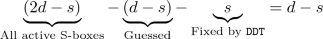
  unused active Sboxes, which are used as a $2^{-(d-s)c}$-bit filter. In Algorithm 2, it is a filter of $2^{-(d-s)c}=2^{-(4-3)\times 8}=2^{-8}$. Once it passes the filter, we obtain the full (A, D) and ($A',D'$) conform to the differential of the SSB.

The complexity of the whole procedure is s DDT accesses and $4(d-s)$ S-boxes evaluations ($2(d-s)$ in step 2 and $2(d-s)$ in step 6). We have to repeat for $2^{(d-s)c}\times 2^{s}$ times to traverse the initial guesses and s-bit auxiliary variable $\beta$ to find one pair on average, which need about $2^{(d-s)c+s} \cdot s$ $\mathtt {DDT}$ accesses and $2^{(d-s)c+s} \cdot 4(d-s)$ small S-box evaluations. Suppose one DDT access is equivalent to one S-box evaluation, hence the total time complexity is in classical setting:

$$\begin{aligned} 2^{(d-s)c+s} \cdot (s+4(d-s)) ~~\text {S-box evaluations}. \end{aligned}$$

(5)

In quantum setting, we use Grover’s algorithm to accelerate the procedures with time complexity (including uncomputing):

$$\begin{aligned} 2\cdot \frac{\pi }{4}\cdot \sqrt{2^{(d-s)c+s}}\cdot (s+4(d-s)) ~~\text {S-box evaluations}, \end{aligned}$$

(6)

with $2^{16}$ qRAM to store the DDT. We refer the readers to Sect. 4 and 5 to find the detailed definitions and implementations of quantum oracles for the application of Grover’s algorithm. From the Eq. (5) and (6), we see that the dominating part is $2^{(d-s)c}$ (in this paper, $c=8$), hence, we will maximize s by our MILP model in order to reduce the complexity to compute the non-full-active super S-box.

3.2 Searching for Exploitable Differentials in Classical and Quantum Attacks with MILP

Following recent MILP based approach for automatic cryptanalysis  [37, 46], we propose an MILP model with multiple optimization objectives whose solution space captures the set of exploitable differentials with respect to rebound attacks in both the classical and quantum settings. Let us now clarify the variables, constraints, and objective functions.

Variables and Constraints. For an R-round primitive, we first introduce an integral variable l, which determines the inbound part from round $l+1$ to round $l+2$, and the outbound part with a backward chunk from round l to round 0 and a forward chunk from round $l+3$ to round $R-1$.

Then, we introduce a set of 0–1 variables $x_j$ for all cells of the states involved, where $x_j = 1$ if and only if the corresponding cell is differentially active. These variables model the truncated differential trails of the target, and the constraints imposed on them are the same as  [37].

To capture the probability of the trails, we also introduce a set of 0–1 variables $\omega _j$ for each cell of the states right before (in the backward chunk) or after (in the forward chunk) the MC operations. Concretely, in the backward chunk, given MC with differentially active input-output cells, $\omega _j = 1$ if and only if the corresponding input cell of the MC is differentially inactive. Similarly, in the forward chunk, given MC with differentially active input-output cells, $\omega _j = 1$ if and only if the corresponding output cell of the MC is differentially inactive. Therefore, the probability of the truncated differential trail for the outbound phase can be calculated as $2^{- c \cdot \sum \omega _j}$, where c is the cell size in bits and the sum of $\omega _j$ is taken over the scope of the outbound part.

The Objective Functions. To minimize the time complexity of the outbound phase (including the cancellation introduced by Eq. (4)), our first priority objective function is to minimize

$$\small \sum _{\mathrm {Outbound}} w_j + \sum _{\mathrm {Round}~0} x_j.$$

According to the discussion of Sect. 3.1, the complexity for analyzing one super S-box is minimized when the number of inactive small S-boxes is maximized. Assuming we have h super S-boxes, let $s_i$ ($0 \le i < h$) denote the number of inactive small S-boxes in the corresponding super S-box. We set our second priority objective function to maximize the minimal of $\{s_0, s_1, ..., s_{h-1}\}$, i.e., the objective function is

$$\mathtt{maximize}:\mathtt{min}~\{s_0, s_1, ..., s_{h-1}\}.$$

Note that this type of objective can be realized in MILP by maximizing $\lambda$ with the constraints $\lambda \le s_j$ for $0 \le j < h-1$.

Remark. Since in all of our attacks we have enough degrees of freedom potentially borrowed from other message blocks, we do not care about the degrees of freedom provided by the inbound differential.

4 Quantum Collision Attacks on 7-Round AES-MMO and AES-MP with Low qRAM

Before we dive into the details of the attack with low qRAM, we would like to give some high-level remarks on the difference between our attack and Hosoyamada and Sasaki’s attack  [20]. The differentials used in  [20] and our attack are presented in Fig. 3 and Fig. 5, respectively. We can see that both differentials cover seven rounds of AES, and the probabilities of the segments of the differentials covering the outbound phases are both $2^{-80}$¹. The main difference appears in the inbound phases: The differential employed by Hosoyamada and Sasaki (see Fig. 3) activates all cells of the super S-boxes involved in the inbound phase while the differential we used gives rise to non-full-active super S-boxes. This discrepancy is the core reason for the reduction of the qRAM usage and brings some technical difficulties preventing us from applying Hosoyamada and Sasaki’s attack directly.

Fig. 5.

The differential trail used in our quantum collision attack on 7-round AES-MMO

Fig. 6.

The framework of the collision attacks with two message blocks

Since the differential probability of the outbound phase is $2^{-80}$, we have to generate about $2^{80}$ starting points to find a collision. If we follow Hosoyamada and Sasaki’s strategy and try to produce a collision for $h = \mathtt {CF}(m, IV)$ with one message block by a rebound attack based on the differential given in Fig. 5, we are doomed to fail due to an inherent shortage of enough starting points. Let us look at the differential trail (see Fig. 5) for the inbound part. There are $2^{8 \times 4}$ possibilities for $\varDelta Z_2$ and $2^{8 \times 3}$ possibilities for $\varDelta W_4$. Therefore, we expect to have totally $2^{8 \times 4} \times 2^{8 \times 3} = 2^{56} < 2^{80}$ starting points when the subkeys are fixed by the IV. In contrast, Hosoyamada and Sasaki’s trail (see Fig. 3) can create as many as $2^{8 \times 8} \times 2^{8 \times 3} = 2^{88} > 2^{80}$ starting points that conforming with the inbound differential.

To address this issue, we consider collisions produced by a pair of two-block messages $(m_0, m_1)$ and $(m_0, m_1')$ whose hash values are computed according to Fig. 6. The rebound attack happens at the second message block, and the degrees of freedom for generating starting points is replenished by varying the first message block $m_0$. To be more specific, we can generate about $2^{24} \times 2^{56} = 2^{80}$ starting points after go through $2^{24}$ different $m_0$’s, among which we expect to find one starting point fulfilling the outbound differential and thus leading to a collision.

4.1 A Low-qRAM Quantum Collision Attack on 7-Round AES-MMO

Similar to [20], at the core of our attack is the application of Grover’s algorithm to a search space where the interested elements are marked by an efficiently computable Boolean function F. Now, let us proceed to define our F.

For the convenience of discussion, we call the instantiated input-output difference pair $(\varDelta _{in}, \varDelta _{out}) \in \mathbb {F}_2^{32} \times \mathbb {F}_2^{24}$ for $(\varDelta X_3, \varDelta Y_4)$ with regard to Fig. 5 the inbound differential. The goal of the inbound phase of a rebound attack is to generate data pairs respecting the inbound differential. We define

$$\begin{aligned} F : \mathbb {F}_2^{24} \times \mathbb {F}_2^{32} \times \mathbb {F}_2^{24} \times \mathbb {F}_2^3 \rightarrow \mathbb {F}_2 \end{aligned}$$

(7)

in a way such that $F(m_0, \varDelta _{in}, \varDelta _{out}, \alpha ) = 1$ if and only if the starting point computed with $(m_0, \varDelta _{in}, \varDelta _{out})$ and indexed by $\alpha = (\alpha _0, \alpha _1, \alpha _2) \in \mathbb {F}_2^3$ fulfills the outbound differential.² Note that we can set the search space of $m_0$ to be the most significant 24 bits, with its remaining bits set to 0. Therefore, if $F(m_0, \varDelta _{in}, \varDelta _{out}, \alpha ) = 1$, we can produce two messages $m_1$ and $m_1'$ with the help of Algorithm 2 such that

$$ \mathtt {CF}(m_1, \mathtt {CF}(m_0, IV)) = \mathtt {CF}(m_1', \mathtt {CF}(m_0, IV)),$$

where $m_1$ and $m_1'$ are obtained from the starting point indexed by $\alpha$. Given $(m_0, \varDelta _{in}, \varDelta _{out}, \alpha )$, $F(m_0, \varDelta _{in}, \varDelta _{out}, \alpha )$ can be computed in the classical world by the following approach:

• 1. Compute $h_1=\mathtt{CF} (m_0,IV)$, which is treated as the master key for the second block encryption.

• 2. Compute the differential $(\varDelta X_{3}^{(i)}, \varDelta Y_{4}^{(i)})$ for each super S-box $\mathtt{SSB} ^{(i)}$ ($0 \le i < 4$) from the inbound differential $(\varDelta _{in},\varDelta _{out})$. Note that the differential trail for $\mathtt{SSB} ^{(0)}$ with input difference $\varDelta X_{3}^{(0)}$ and output difference $\varDelta Y_{4}^{(0)}$ is highlighted in Fig. 5.

• 3. Solve the non-full active super S-box $\mathtt{SSB} ^{(0)}$ to obtain $X_3^{(0)}$ such that

  $$\mathtt{SSB} ^{(0)}(X_3^{(0)} \oplus \varDelta X_3^{(0)} ) \oplus \mathtt{SSB} ^{(0)}(X_3^{(0)} ) = \varDelta Y_4^{(0)}.$$

  If $\alpha _0=0$, pick $\mathtt {min} \{X_{3}^{(0)}, X_{3}^{(0)} \oplus \varDelta X_{3}^{(0)}\}$ as the new value for $X_{3}^{(0)}$. Else, pick $\mathtt {max} \{X_{3}^{(0)}, X_{3}^{(0)} \oplus \varDelta X_{3}^{(0)}\}$ as the new value for $X_{3}^{(0)}$. Similarly, we obtain $X_3^{(1)}$, $X_3^{(2)}$. For the pair $(X_3^{(3)}, X_3^{(3)}\oplus \varDelta X_3^{(3)})$, we always pick the bigger one as $X_3^{(3)}$. We can build the starting point

  $$ X_3 = (X_3^{(0)}, X_3^{(1)}, X_3^{(2)}, X_3^{(3)} ) $$

  according to the index $\alpha$.

• 4. If the starting point $(X_3, X_3 \oplus \varDelta X_3)$ obtained in step 3 respects the outbound differential, $F(m_0,\varDelta _{in},\varDelta _{out}, \alpha )$ returns 1, otherwise it returns 0.

Therefore, by applying Grover’s search with the quantum oracle $\mathcal {U}_F$ which maps to , we can find a collision with around $\frac{\pi }{4} \cdot \sqrt{2^{83}}$ queries. To estimate the overall complexity, we need to be clear on the complexity incurred by $\mathcal {U}_{F}$.

4.2 Implementation of the Quantum Oracle $\mathcal {U}_{F}$

Similar to  [20], we need some additional functions to implement $\mathcal {U}_F$. First, we define $G^{(i)}$, which marks the values of one byte of $X_3^{(i)}$ and a 3-bit index $\beta$ leading to solutions (compatible data pairs) for the given differential $(\varDelta X_{3}^{(i)}, \varDelta Y_{4}^{(i)})$ of the super S-box $\mathtt{SSB} ^{(i)}$ and an initial message block $m_0$ when Algorithm 2 or its variants are applied. For example, $G^{(0)}(m_0,\varDelta X_{3}^{(0)}, \varDelta Y_{4}^{(0)}, X_{3}^{(0)}[0], \beta ) = 1$ if and only if we pass the check in Step 19 of Algorithm 2 upon input of $(m_0,\varDelta X_{3}^{(0)}, \varDelta Y_{4}^{(0)}, X_{3}^{(0)}[0], \beta )$. Note that, since $G^{(0)}$ is just to mark the correct 11-bit $(X_{3}^{(i)}[0], \beta )$ for a given $(m_0,\varDelta X_{3}^{(0)}, \varDelta Y_{4}^{(0)})$, we can return $G^{(0)}=1$ once it passes the check in Step 19 of Algorithm 2.

Since the computation of $G^{(i)}$ in the classical setting uses the table $\mathbb {T}$ computed by Algorithm 1, implementing a quantum oracle of $G^{(i)}$ requires qRAMs. The implementation of the quantum oracle $\mathcal {U}_{G^{(0)}}$ of $G^{(0)}$ is presented in Algorithm 3.

For $0\le i < 3$, we use the function $D^{(i)}$ to compute the actual input-output data pair respecting the differential of the super S-box $\mathtt{SSB} ^{(i)}$ with the knowledge of one byte of $X_{3}^{(i)}[0]$ and $\beta$ obtained by executing Grover search on $G^{(i)}$. $D^{(i)}$ is just to replay a full version of Algorithm 2 and outputs $\mathtt {min} \{X_{3}^{(i)}, X_{3}^{(i)} \oplus \varDelta X_{3}^{(i)}\}$ upon input

$$(m_0,\varDelta X_{3}^{(i)}, \varDelta Y_{4}^{(i)}, X_{3}^{(i)}[0],\beta ;\alpha _{i} = 0),$$

and outputs $\mathtt {max} \{X_{3}^{(i)}, X_{3}^{(i)} \oplus \varDelta X_{3}^{(i)}\}$ upon input

$$(m_0,\varDelta X_{3}^{(i)}, \varDelta Y_{4}^{(i)}, X_{3}^{(i)}[0],\beta ;\alpha _{i} = 1),$$

such that $\mathtt{SSB} ^{(i)}(X_{3}^{(i)})\oplus \mathtt{SSB} ^{(i)}(X_{3}^{(i)} \oplus \varDelta X_{3}^{(i)})=\varDelta Y_{4}^{(i)}$. In addition, $D^{(3)}$ is defined differently. It always returns the smaller one of $X_{3}^{(3)}$ and $X_{3}^{(3)} \oplus \varDelta X_{3}^{(3)}$ upon the input $(m_0,\varDelta X_{3}^{(i)}, \varDelta Y_{4}^{(i)}, X_{3}^{(i)}[0],\beta )$, such that

$$\mathtt{SSB} ^{(3)}(X_{3}^{(3)})\oplus \mathtt{SSB} ^{(3)}(X_{3}^{(3)} \oplus \varDelta X_{3}^{(3)})=\varDelta Y_{4}^{(3)}.$$

Finally, the oracle $\mathcal {U}_F$ can be constructed by using $\mathcal {U}_{G^{(i)}}$ and the quantum circuits of $D^{(i)}$ which is presented in Algorithm 4.

Complexity Analysis. To produce fair and comparable results, the assumptions made by Hosoyamada and Sasaki  [20] are inherited in our complexity analysis:

• The complexity of the computation of 7-round AES is approximated by $16 \times 7$ + $4 \times 7 = 140$ S-box computations.

• The complexity of one access to the qRAM storing a table is equivalent to one S-box computation.

• The complexity of the resolution of the linear equation involving $\mathtt {MC}$ with four knowns and four unknowns is equivalent to one $\mathtt {MC}$ operation and is ignored.

• One inverse Sbox is about two Sboxes [21].

• Uncomputing is taken into account.

First of all, in our attack, the differential distribution table with $2^{16}$ classical data for the S-box is precomputed (see Algorithm 1) and loaded into a qRAM in advance, which is accessed by the quantum circuits for $G^{(i)}$ and $D^{(i)}$.

Complexity of the Grover Search on $G^{(i)}$. Applying Grover algorithm to $G^{(i)}$ given $(m_0,\varDelta X_{3}^{(i)}, \varDelta Y_{4}^{(i)})$ to find a 11-bit value $(X_{3}^{(i)}[0], \beta ^{(i)})$ requires $\frac{\pi }{4}\sqrt{2^{8+3}} \approx 2^{5.15}$ queries to the oracle $\mathcal {U}_{G^{(i)}}$³. According to the analysis of Algorithm 2, one query to $\mathcal {U}_{G^{(i)}}$ takes about $s=3$ qRAM accesses and $4(d-s)=4(4-3)=4$ S-box evaluations, the overall complexity can be estimated as $2\times 2^{5.15} \times (3+4) \times \frac{1}{140} \approx 2^{1.83}$ 7-round AES computations.

Complexity of $D^{(i)}$. $D^{(i)}$ is just to replay a full version of Algorithm 2. In Step 1–19 of Algorithm 2, it needs $s+4(d-s)=3+4(4-3)=$7 S-boxes evaluations. In Step 21, since all the 5 active bytes are known before, we just compute the last 3 inactive Sboxes (see Fig. 4) to determine a conforming pair for the $\mathtt{SSB} ^{(i)}$. Hence, totally 7 + 3 = 10 Sboxes evaluations are needed, which is about $2\times \frac{10}{140} \approx 2^{-2.8}$ 7-round AES computations.

Complexity of $\mathcal {U}_F$. In Algorithm 4, Step 1 needs one 7-round AES computation; Step 2–9 need $4 \times (2^{1.83}+2^{-2.8}) \approx 2^{3.88}$ 7-round AES computations. In Step 13, according to Fig. 5, we need to compute backward for 2 rounds and forward for 3 rounds from the starting point $(X,X')$. Therefore, $2\times 2\times 16=64$ inverse Sboxes and $2\times 3\times 16=96$ Sboxes are needed, which are equal to $2\times \frac{64\times 2+96}{140}=3.2$ 7-round AES computations. Totally, the complexity of $\mathcal {U}_F$ is $1+2^{3.88}+3.2\approx 2^{4.24}$ 7-round AES computations. Supplementary Material D of the full version of the paper at https://eprint.iacr.org/2020/1030 discusses the success probability of $\mathcal {U}_F$.

Complexity to Find a Collision. To identify an 83-bit value $(m_0,\varDelta _{in},\varDelta _{out}, \alpha ) \in \mathbb {F}_2^{24} \times \mathbb {F}_2^{32} \times \mathbb {F}_2^{24} \times \mathbb {F}_2^{3}$ with Grover search such that $F(m_0, \varDelta _{in}, \varDelta _{out}, \alpha )=1$ requires about $\frac{\pi }{4}\times \sqrt{2^{83}}$ queries to $\mathcal {U}_{F}$. Therefore, the complexity to find a collision is $\frac{\pi }{4}\times \sqrt{2^{83}} \times 2^{4.24} =2^{45.4}$ 7-round AES computations.

5 Quantum Attacks on 7-Round AES-MMO Without qRAM

The qRAM dependence of the previous attack comes from the qRAM dependence of $\mathcal {U}_{ G^{(i)} }$ and ${ D^{(i)} }$. To get rid of the qRAMs, we re-implement $\mathcal {U}_{ G^{(i)} }$ and $D^{(i)}$ without using the DDT stored in qRAMs, while keep their functional behavior unchanged. In this section, we introduce two method to reduced qRAMs to zero.

Method 1. The idea is simple: given a differential of an $8 \times 8$ S-box, data pairs are generated by on-line search instead of table lookups. Since the methods for re-implementing $\mathcal {U}_{ G^{(i)} }$ and $D^{(i)}$ are similar, we only give the details of the implementation of $\mathcal {U}_{ G^{(0)} }$ in Algorithm 5. The complexity analysis of this new attack is given in the following.

Complexity of the Grover Search on $G^{(i)}$. Applying Grover’s algorithm to $G^{(i)}$ given $(m_0,\varDelta X_{3}^{(i)}, \varDelta Y_{4}^{(i)})$ to find a 11-bit value $(X_{3}^{(i)}[0], \beta ^{(i)})$ requires $\frac{\pi }{4}\sqrt{2^{8+3}} \approx 2^{5.15}$ queries to the oracle $\mathcal {U}_{G^{(i)}}$. According to Algorithm 5, the complexity of one query to $U_{G^{(i)}}$ is dominated by Step 6–8, which is about $3\cdot \frac{\pi }{4}\cdot \sqrt{2^8}\cdot (\frac{1}{140})=2^{-1.89}$ 7-round AES. Hence, the total complexity of the Grover search on $G^{(i)}$ is about $2\times 2^{5.15}\times 2^{-1.89}=2^{4.27}$ 7-round AES.

Complexity of $D^{(i)}$. With $(X_{3}^{(i)}[0], \beta ^{(i)})$, $D^{(i)}$ outputs the pair respecting the differential of the super S-box on-line. The implementation of $D^{(i)}$ is similar to $G^{(i)}$, with Step 12–14 of Algorithm 5 replaced by outputting $X_3^{i}$ according to $\alpha _i$ (please refer the definitions of $D^{(i)}$ in Sect. 4.2 for details). The complexity of $D^{(i)}$ is also bounded by Step 6–8 of Algorithm 5. The complexity is about $2\times 2^{-1.89}=2^{0.89}$ 7-round AES.

Complexity of $\mathcal {U}_F$. The implementation of $\mathcal {U}_F$ without qRAM is obtained by replacing $G^{(i)}$ and $D^{(i)}$’s with their no-qRAM versions (Algorithm 4). The complexity of one query to $\mathcal {U}_{F}$ is about $4\times (2^{4.27}+2^{-0.89})+1+3.2\approx 2^{6.384}$ 7-round AES computations.

Complexity to Find a Collision. To identify an 83-bit value $(m_0,\varDelta _{in},\varDelta _{out}, \alpha ) \in \mathbb {F}_2^{24} \times \mathbb {F}_2^{32} \times \mathbb {F}_2^{24} \times \mathbb {F}_2^{3}$ with Grover search such that $F(m_0, \varDelta _{in}, \varDelta _{out}, \alpha )=1$ requires about $\frac{\pi }{4}\times \sqrt{2^{83}}$ queries to $\mathcal {U}_{F}$. Therefore, the complexity to find a collision is $\frac{\pi }{4}\times \sqrt{2^{83}} \times 2^{6.384} =2^{47.584}$ 7-round AES computations.

Method 2. At FSE 2020, Bonnetain, Naya-Plasencia and Schrottenloher [4] introduced a quantum circuit that fulfilled the functionality of DDT. The cost is equivalent to 2 Sboxes computations and 22 ancilla qubits. In this section, we use this idea to implement $\mathcal {U}_F$ without qRAMs. The complexity is quit similar to Algorithm 4, since when one DDT access is needed, we just replace it by 2 Sbox evaluations. The updated complexity of $G^{(i)}$ is $2s+4(d-s)=6+4=10$ Sbox evaluations. Therefore, applying Grover’s algorithm to $G^{(i)}$ costs $2\times 2^{5.15}\times 10 \times \frac{1}{140}\approx 2^{2.34}$ 7-round AES. The complexity of $D^{(i)}$ is about $2\times \frac{13}{140}\approx 2^{-2.43}$ 7-round AES. Hence, the complexity of $\mathcal {U}_F$ becomes $1+4\times (2^{2.34}+2^{-2.43})+3.2\approx 2^{4.66}$ 7-round AES. Totally, we need $\frac{\pi }{4}\times \sqrt{83}\times 2^{4.66}\approx 2^{45.8}$ 7-round AES computations with 22 ancilla qubits.

6 Collision Attacks on Grøstl-512

Grøstl is a SHA3 finalist hash function. It comes with two versions: Grøstl-256 and Grøstl-512, with the trailing digits signifying the sizes of the outputs in bits. The structure of Grøstl-$\frac{n}{2}$ with two message blocks is depicted in Fig. 7, where P and Q are two n-bit AES-like permutations. Before it outputs the hash value, an output transformation based on P and a truncation $\varOmega : \mathbb {F}_2^n \rightarrow \mathbb {F}_2^{n/2}$ are applied to $h_2$. We refer the reader to  [11] for more details of the design.

Fig. 7.

Grøstl-$\frac{n}{2}$ with two message blocks

The best known collision attack on Grøstl-512 reaches 3 rounds  [43]. Based on differentials found by MILP technique, we present the first classical and dedicated quantum collision attacks on 4-round and 5-round Grøstl-512. To facilitate our discussion, we use the alternative but equivalent description of Grøstl introduced by  [34], which is illustrated in Fig. 8. Let $P^-$ and $Q^-$ be the AES-like permutations with their last MB operations removed. We have the following equivalent description of Grøstl. For $1 \le i \le t$, we set

$$\begin{aligned} \begin{aligned}&v_{0} = \mathtt{MB}^{-1}(IV),\\&v_{i} = P^-(\mathtt{MB}(v_{i-1})\oplus m_{i-1})\oplus Q^-( m_{i-1})\oplus v_{i-1},\\&h=\varOmega (\mathtt{MB}(v_{t})). \end{aligned} \end{aligned}$$

Fig. 8.

An alternative description of Grøstl-$\frac{n}{2}$ with two message blocks

6.1 Exploitable Differential Trails of Grøstl-512

The differential trails we used in our collision attacks on Grøstl-512 are inspired by Mendel, Rijmen and Schläffer’s collision attack on 4-round Grøstl-256  [34]. In  [34], a random difference is injected through $m_0$ to create a fully differentially active chaining value $v_1$. Then a sequence of local rebound attacks is performed to cancel the differences in the chaining values “column” by “column”, which eventually leads to a full collision. The differential trails employed to trigger such cancellations are shown in Fig. 11 in the Supplementary Material A of the full version of the paper at https://eprint.iacr.org/2020/1030.

However, if we adopt a series of similar differential trails in the attack on 4-round Grøstl-512, we end up with impossible differentials (see Fig. 12 in the Supplementary Material A of the full version of the paper for examples) such that the cancellation of the last “column” never happens. To overcome this difficulty, we have to cancel multiple “columns” at once during the rebound attack over the final message block, which increases the time complexity significantly. To minimize the complexity penalty due to the multiple-column cancellation, we apply the MILP model to the last two steps to find two truncated differential trails to cancel the differences in the last two chaining values before the collision. The identified trails are depicted in Fig. 13 in the full version of the paper, where in the last step we attempt to cancel 16 active bytes at once, and the numbers of inactive S-boxes for the 16 super S-boxes SSB of the inbound phase (see Fig. 9) are given as $(s_0, s_1, \cdots , s_{15}) = (7, 7, 6, 7, 7, 7, 5, 3, 4, 4, 4, 4, 4, 4, 5, 7).$

6.2 Classical and Quantum Collision Attacks on 4-Round Grøstl-512

Based on the differential trails given in Fig. 13 in Supplementary Material A of the full version of the paper, a classical collision attack on 4-round Grøstl-512 can be constructed. The strategy of the attack generally follows the strategy of  [34] with a critical difference at the initial difference injection. The attack of  [34] starts with an arbitrary fully active chaining value $v_1$. In our attack, we impose additional conditions on the fully active chaining value $v_1$. We now clarify these conditions.

From Fig. 13 of the full version of the paper we can see that for a fixed initial pair of message blocks $(m_0, m_0')$, the difference of the cells of the chaining states $v_i$ keeps unchanged throughout the entire attack unless they are canceled. Therefore, to force the chaining values following the specified differential trails for the last two-column cancellation, we can pretest some cells of $\varDelta v_1$, which are marked by blue cells in Fig. 13, and the required differential transformation is depicted in Fig. 9.

Fig. 9.

The inbound phase of the last step of the collision attack on Grøstl-512. The gray and blue bytes are active, but there are conditions on blue bytes. The green bytes are inactive due to the conditions imposed on the blue cells. (Color figure online)

Specifically, we introduce some conditions on some active bytes (marked by blue) within some columns in the chaining values. For example, in $v_{i-1}$ of Fig. 13, there are 10 blue bytes. In the first column of $v_{i-1}$, the two active blue bytes have to meet the condition for the differential propagation:

Similar conditions for other blue bytes in the other 4 columns are also needed. For randomly selected pair $(m_0,m'_0)$, the output difference $\varDelta v_1$ meets the conditions in the blue bytes with probability $2^{-8\times 5}=2^{-40}$. Hence, with $2^{40}$ $(m_0,m'_0)$ pairs, we are expected to find one correct pair.

In summary, this attack starts with a fully differentially active $v_1$ fulfilling the required conditions by injecting a random difference at $m_0$, repeats local rebound-like attacks over the subsequent message blocks to cancel the differences column by column until there are only two differentially active columns, and a final rebound attack is employed to cancel the last two active columns as a whole. The colliding pair is of the form: $M = (m_0, m_1, \cdots , m_t)$ and $M' = (m_0', m_1, \cdots , m_t)$, that is, only the starting message block $m_0$ has a difference. The procedure of the attack is outlined in the following.

• 1. Choose arbitrary $2^{40}$ message blocks $m_0$, $m'_0$ and compute the difference $\varDelta v_1 = v_1 \oplus v_1'$ with conditions on five columns satisfied in the blue bytes. Since the probability is $2^{-40}$ for a random pair ($m_0$, $m'_0$), we are expected to find one right pair.

• 2. Perform rebound attacks over the message block $m_1$. Note that the input difference $\varDelta _{in}$ of the inbound phase is fixed due to $\varDelta v_1$, and the output difference $\varDelta _{out}$ of the inbound phase has 8 active cells as shown in Fig. 13. Using the full-active-super S-box technique⁴, we can generate $2^0 \times 2^{64} = 2^{64}$ messages $m_1$ (starting points) such that the pair $(m_1 \oplus \mathtt {MB}(v_1), m_1 \oplus \mathtt {MB}(v_1'))$ respect the given inbound differential. With regards to the outbound differential, the truncated differential ($8\rightarrow 8\rightarrow 8$) given in Fig. 13 holds with probability 1, and the 8-bytes cancellation due to the feed-forward exclusive-or happens with probability $2^{-64}$. Therefore, we expect one of $2^{64}$ starting points to fulfill the one-column local collision, and the time complexity of this step is about $2^{64}$.

• 3. Repeat step 2 with the corresponding differential trails to inactivate the differences of the chaining values column by column until only two active columns remain.

• 4. Eliminate the last two active columns with the same strategy of step 2. Since there are 16 active bytes in the output difference of the inbound differential, we can obtain $2^{16 \times 8} = 2^{128}$ starting points with time complexity $2^{128}$ by using the super S-box technique. With regard to the outbound differential, the truncated differential $16\rightarrow 16\rightarrow 16$ holds with probability 1, and the two-column cancellation happens with probability $2^{-128}$. Therefore, we can obtain the desired collision with $2^{128}$ starting points.

The time complexity of the attack is dominated by Step 4 of the above procedure, which is about $2^{128}$. The storage of the super-Sbox leads to a memory complexity of $2^{64}$. Finally, we find a collision for the 4-round Grøstl-512 with about 16 message blocks. A quantum version of the same attack on 4-round Grøstl-512 with or without qRAMs can be constructed based on the same method given in Sect. 4 and Sect. 5, and we refer the reader to Supplementary Material B of the full version of the paper at https://eprint.iacr.org/2020/1030 for the details.

6.3 Classical and Quantum Collision Attacks on 5-Round Grøstl-512

The 4-round collision attack can be extended to a 5-round collision attack shown in Fig. 14 in Supplementary Material A of the full version of the paper, where the probabilities of the outbound phases of the rebound attacks are $2^{-56}$ and $2^{-112}$ (the last step). When a local rebound attack fails to produce the local collision on a column, we will perform the same attack on the next message block until the desire difference cancellations occur. Therefore, how many message blocks are used in the attack is unknown before we reach a full collision. We briefly summarize the attack on 5-round Grøstl-512 below:

• 1. Choose arbitrary message blocks $m_0$, $m'_0$ and compute the difference $\varDelta v_1 = v_1 \oplus v_1'$ until the required conditions on the blue cells are satisfied. We are expected to find one correct pair after $2^{40}$ repetitions.

• 2. Perform rebound attacks over the message block $m_1$. Note that the input difference $\varDelta _{in}$ of the inbound phase is fixed due to $\varDelta v_1$, and the output difference $\varDelta _{out}$ of the inbound phase has 8 active cells. Using the full-active super S-box technique, we can generate $2^0 \times 2^{64} = 2^{64}$ messages $m_1$ (starting points). With regards to the outbound differential, the truncated differential ($128\rightarrow 64\rightarrow 8\rightarrow 1\rightarrow 8\rightarrow 8$) holds with probability $2^{-56}$, and the 8-bytes cancellation due to the feed-forward exclusive-or happens with probability $2^{-64}$. Therefore, we can obtain the desired difference for the chaining value with probability $2^{64} \times 2^{-56} \times 2^{-64} = 2^{-56}$ with $2^{64}$ time complexity. If we are failed to get the desired difference, we perform the same attack over the next message block with the chaining values produced previously. We will succeed in canceling the 8-byte difference after about $2^{56}$ additional message blocks are processed.

• 3. Repeat step 2 with the corresponding differential trails to inactivate the differences of the chaining values column by column until only two active columns remain.

• 4. Eliminate the last two active columns with the same strategy of step 2. The success probability of the local rebound attack performed in this step is different from others. Since there are 16 active bytes in the output difference of the inbound differential, we can obtain $2^{16 \times 8} = 2^{128}$ starting points with time complexity $2^{128}$ by using the super S-box technique. With regard to the outbound differential, the truncated differential trail $88\rightarrow 96\rightarrow 16\rightarrow 2\rightarrow 16\rightarrow 16$ holds with probability $2^{-112}$, and the two-column cancellation happens with probability $2^{-128}$. Therefore, we can obtain the desired collision with probability $2^{128} \times 2^{-112} \times 2^{-128} = 2^{-112}$ with $2^{128}$ time complexity (within this step). If we fail to get the collision, repeating Step 4 with about $2^{112}$ additional message blocks will achieve the collision.

The time complexity of the attack is dominated by step 4, which can be estimated as $2^{112} \times 2^{128} = 2^{240}$. The storage of the super S-box leads to a memory complexity of $2^{64}$. Finally, we find a collision with about $2^{112}$ message blocks. A quantum version of the same attack can be constructed, which is quite similar to the attack given in Supplementary Material B of the full version of the paper. We repeat a quantum version of Step 4 for $2^{112}$ times to find a collision. The time complexity of the quantum attack with $2^{16}$ qRAMs is $2^{88.37}\times 2^{112}=2^{200.4}$, and the time complexity of the quantum attack without qRAMs is $2^{89.3}\times 2^{112}=2^{201.3}$.

7 Semi-Free-Start Collision Attacks on Grøstl-256

So far, the best collision attack on 6-round Grøstl-256 is a semi-free-start collision attack with time complexity $2^{120}$ and memory complexity $2^{64}$. Based on the truncated differential trail covering 6-round Grøstl-256 found by the MILP technique, which is depicted in Fig. 10, we can improve this attack in both the classical and quantum settings.

Fig. 10.

Differential trail of the compression function of 6-round Grøstl-256

The Classical Attack. Two rebound attacks are applied to P and Q separately. The inbound phase of the rebound attack on P begins at $P_2$ and ends at $P_4$. There are $2^{56} \times 2^{56}=2^{112}$ input-output differences in total, and we expect to find $2^{112}$ starting points with $2^{112}$ time complexity based on the super S-box technique. In the outbound phase, the probability for fulfilling the outbound truncated differential trail is $2^{-48}\times 2^{-48}=2^{-96}$. Therefore, we can produce $2^{112}\times 2^{-96}=2^{16}$ pairs respecting the 6-round truncated differential covering P with time complexity $2^{112}$. Similarly, performing a rebound attack with time complexity $2^{112}$ over Q generates $2^{16}$ pairs respecting the truncated differential trail covering Q. Combining the results of the two rebound attacks, we obtain $2^{16} \times 2^{16}=2^{32}$ quartets $((P_0,P'_0), (Q_0,Q'_0))$, among which we expect to identify $2^{32} \times 2^{-16} \times 2^{-16} = 1$ quartet such that $\varDelta Q_0 = \varDelta P_0$ and $\varDelta P_6 = \varDelta Q_6$. This leads to a semi-free-start collision with $m_{i-1} = Q_0$, $m'_{i-1} = Q'_0$, and $h_{i-1} = Q_0\oplus P_0=Q'_0\oplus P'_0$. The time complexity of the attack about $2^{112}$, and we need $2^{64}$ memory to apply the super S-box technique.

The Quantum Attack Without qRAMs. The quantum attack is also based on the differential trails shown in Fig. 10. Given an inbound differential $(\varDelta _{in}^{P},\varDelta _{out}^{P}) \in \mathbb {F}_2^{56} \times \mathbb {F}_2^{56}$ for the permutation P. If there is a starting point respecting the given inbound differential, then one can generate $2^{7}$ different starting points, which are indexed by $\alpha _P \in \mathbb {F}_2^{7}$. We define $F_P : \mathbb {F}_2^{56} \times \mathbb {F}_2^{56} \times \mathbb {F}_2^{7} \rightarrow \mathbb {F}_2$ such that $F_P(\varDelta _{in}^{P},\varDelta _{out}^{P}, \alpha _P) = 1$ if and only if there is a starting point respecting the inbound differential $(\varDelta _{in}^{P},\varDelta _{out}^{P})$ and the particular starting point indexed by $\alpha _P$ also conforming with the outbound differential of P. The probability of the outbound phase is $2^{-48-48}=2^{-96}$. Therefore, given $(\varDelta _{in}^{P},\varDelta _{out}^{P},\alpha _P)$, $F_P(\cdot )$ return 1 with probability of $2^{-96-7}=2^{-103}$.

Applying Grover algorithm with certainty to the quantum oracle $\mathcal {U}_{F_P}$ which is constructed without qRAM with similar techniques shown in previous sections, we can obtain a superposition

(8)

where $\sqrt{ \{ x \in \mathbb {F}_2^{119}: F_P(x) = 1 \} } \approx \sqrt{2^{56} \times 2^{56}\times 2^7 \times 2^{-103}} \approx \sqrt{2^{16}}$.

As shown in the generalized version of Algorithm 2, given parameters ($d=8,c=8,s$), where s is the sum of the non-active bytes of the input-output differential of the non-full-active super S-box, we have to traverse $2^{(d-s)c+s}$ to find the conforming pair of super S-box (an s-bit auxiliary variable to specify which value to choose within the pair obtained by accessing s DDT). To find a conforming pair for the super S-box, we also define a similar $G^{(i)}$ as defined in Algorithm 5. According to the Eq. (6), the time complexity to implement $G^{(i)}$ is about $4(d-s)+s$, with s DDT accesses and $4(d-s)$ small Sbox evaluations. Here, we only considering the attack without storing DDT in qRAM. Hence, s DDT accesses become s implementations of Grover algorithm to find a conforming pair for the s S-boxes. Hence, the time complexity to search on $U_{G^{(i)}}$ using Grover algorithm is about

$$\begin{aligned} \small 2\cdot \frac{\pi }{4}\cdot \sqrt{2^{(d-s)c+s}}\cdot (4(d-s)+s\cdot (\frac{\pi }{4}\cdot \sqrt{2^{c}})),~\text {S-box evaluations}. \end{aligned}$$

(9)

Considering the non-full-active super S-boxes in Fig. 10, the sum of non-active Sboxes in each SSB is $s=2$. Hence, to find a conforming pair with given input and output differences of SSB, the time complexity is about $2^{31.27}$ S-box evaluations according to Eq. (9), which is about $2^{31.27}/768=2^{21.68}$ 6-round Grøstl-256 without qRAM.

When applying Grover algorithm to setup $F_P$, we need about $\frac{\pi }{4}\cdot \sqrt{2^{96+7}}\cdot 8\cdot 2^{21.68}\approx 2^{75.8}$ 6-round Grøstl-256 without qRAM to get the desired superposition in Eq. (8).

Similarly, applying Grover search to $F_Q$, where $F_P(\varDelta _{in}^{Q},\varDelta _{out}^{Q}, \alpha _Q) = 1$ if and only if there is a starting point respecting the inbound differential $(\varDelta _{in}^{Q},\varDelta _{out}^{Q})$ and the particular starting point indexed by $\alpha _Q$ also conforming with the outbound differential of Q. With the same complexity of the first Grover search, we obtain a superposition

(10)

where $\sqrt{ \{ x \in \mathbb {F}_2^{119}: F_Q(x) = 1 \} } \approx \sqrt{ 2^{56} \times 2^{56}\times 2^{7} \times 2^{-103}} \approx \sqrt{2^{16}}$.

Now, we are ready to perform the amplitude amplification with $\mathcal {A}$ being the unitary operator sending to and projector , where $\mathbb {C}$ is the set of all $(\varDelta _{in}^{Q},\varDelta _{out}^{Q},\alpha _Q;\varDelta _{in}^{P},\varDelta _{out}^{P},\alpha _P) \in \mathbb {F}_2^{238}$ such that the starting points due to $(\varDelta _{in}^{Q},\varDelta _{out}^{Q},\alpha _Q)$ and ($\varDelta _{in}^{P},\varDelta _{out}^{P},\alpha _P)$ produce a semi-free-start collision. As shown in Fig. 10, the probability that $\varDelta Q_0=\varDelta P_0$ and $\varDelta Q_6=\varDelta P_6$, which lead a collision, is about $2^{-16}\times 2^{-16}=2^{-32}$. The complexity to find a collision without qRAM is $\sqrt{2^{32}}\cdot 2\cdot 2^{75.8}\approx 2^{92.8}$ 6-round Grøstl-256.

8 Conclusion

In this work, we show that the amount of qRAMs required by the quantum attacks on AES-MMO and AES-MP proposed by Hosoyamada and Sasaki can be significantly reduced with only a slight increase in the time complexity. This is achieved by performing a quantum version of the rebound attack based on the non-full-active super S-box technique. Along the way, we find that the non-full-active super S-box analysis can be partially automated with the MILP approach, which is of independent interest, leading to improved attacks on Grøstl in both the classical and quantum settings. To the best our knowledge, our attacks are the first dedicated quantum collision attack on hash functions that slightly outperform Chailloux, Naya-Plasencia, and Schrottenloher’s generic attack (ASIACRYPT 2017) in a model where large qRAMs are not available.

References

Arunachalam, S., Gheorghiu, V., Jochym-O’Connor, T., Mosca, M., Srinivasan, P.V.: On the robustness of bucket brigade quantum RAM. In: TQC 2015, Brussels, Belgium, 20–22 May 2015, pp. 226–244 (2015)
Bonnetain, X., Hosoyamada, A., Naya-Plasencia, M., Sasaki, Y., Schrottenloher, A.: Quantum attacks without superposition queries: the offline Simon’s algorithm. In: Galbraith, S.D., Moriai, S. (eds.) ASIACRYPT 2019, Part I. LNCS, vol. 11921, pp. 552–583. Springer, Cham (2019). https://doi.org/10.1007/978-3-030-34578-5_20
Bonnetain, X., Naya-Plasencia, M., Schrottenloher, A.: On quantum slide attacks. In: Paterson, K.G., Stebila, D. (eds.) SAC 2019. LNCS, vol. 11959, pp. 492–519. Springer, Cham (2020). https://doi.org/10.1007/978-3-030-38471-5_20
Bonnetain, X., Naya-Plasencia, M., Schrottenloher, A.: Quantum security analysis of AES. IACR Trans. Symmetric Cryptol. 2019(2), 55–93 (2019)
Brassard, G., Hoyer, P., Mosca, M., Tapp, A.: Quantum amplitude amplification and estimation. Contemp. Math. 305, 53–74 (2002)
Brassard, G., Høyer, P., Tapp, A.: Quantum cryptanalysis of hash and claw-free functions. In: Lucchesi, C.L., Moura, A.V. (eds.) LATIN 1998. LNCS, vol. 1380, pp. 163–169. Springer, Heidelberg (1998). https://doi.org/10.1007/BFb0054319
Chailloux, A., Naya-Plasencia, M., Schrottenloher, A.: An efficient quantum collision search algorithm and implications on symmetric cryptography. In: Takagi, T., Peyrin, T. (eds.) ASIACRYPT 2017, Part II. LNCS, vol. 10625, pp. 211–240. Springer, Cham (2017). https://doi.org/10.1007/978-3-319-70697-9_8
Daemen, J., Rijmen, V.: The Design of Rijndael: AES - The Advanced Encryption Standard. Information Security and Cryptography. Springer, Heidelberg (2002). https://doi.org/10.1007/978-3-662-04722-4
Damgård, I.B.: A design principle for hash functions. In: Brassard, G. (ed.) CRYPTO 1989. LNCS, vol. 435, pp. 416–427. Springer, New York (1990). https://doi.org/10.1007/0-387-34805-0_39
Dong, X., Dong, B., Wang, X.: Quantum attacks on some Feistel block ciphers. Des. Codes Cryptogr. 88(6), 1179–1203 (2020)
Gauravaram, P., et al.: Grøstl - a SHA-3 candidate. In: Symmetric Cryptography, 11–16 January 2009 (2009)
Gilbert, H., Peyrin, T.: Super-sbox cryptanalysis: improved attacks for AES-like permutations. In: Hong, S., Iwata, T. (eds.) FSE 2010. LNCS, vol. 6147, pp. 365–383. Springer, Heidelberg (2010). https://doi.org/10.1007/978-3-642-13858-4_21
Giovannetti, V., Lloyd, S., Maccone, L.: Architectures for a quantum random access memory. Phys. Rev. A 78(5), 052310 (2008)
Giovannetti, V., Lloyd, S., Maccone, L.: Quantum random access memory. Phys. Rev. Lett. 100(16), 160501 (2008)
Grassi, L., Naya-Plasencia, M., Schrottenloher, A.: Quantum algorithms for the \(k\)-xor problem. In: Peyrin, T., Galbraith, S. (eds.) ASIACRYPT 2018, Part I. LNCS, vol. 11272, pp. 527–559. Springer, Cham (2018). https://doi.org/10.1007/978-3-030-03326-2_18
Grover, L.K.: A fast quantum mechanical algorithm for database search. In: Proceedings of the Twenty-Eighth Annual ACM Symposium on the Theory of Computing, Philadelphia, Pennsylvania, USA, 22–24 May 1996, pp. 212–219 (1996)
Guo, C., Katz, J., Wang, X., Yu, Y.: Efficient and secure multiparty computation from fixed-key block ciphers. IACR Cryptology ePrint Archive 2019, 74 (2019)
Hosoyamada, A., Sasaki, Y.: Cryptanalysis against symmetric-key schemes with online classical queries and offline quantum computations. In: Smart, N.P. (ed.) CT-RSA 2018. LNCS, vol. 10808, pp. 198–218. Springer, Cham (2018). https://doi.org/10.1007/978-3-319-76953-0_11
Hosoyamada, A., Sasaki, Y.: Quantum Demiric-Selçuk meet-in-the-middle attacks: applications to 6-round generic Feistel constructions. In: Catalano, D., De Prisco, R. (eds.) SCN 2018. LNCS, vol. 11035, pp. 386–403. Springer, Cham (2018). https://doi.org/10.1007/978-3-319-98113-0_21
Hosoyamada, A., Sasaki, Y.: Finding hash collisions with quantum computers by using differential trails with smaller probability than birthday bound. In: Canteaut, A., Ishai, Y. (eds.) EUROCRYPT 2020, Part II. LNCS, vol. 12106, pp. 249–279. Springer, Cham (2020). https://doi.org/10.1007/978-3-030-45724-2_9
Jaques, S., Naehrig, M., Roetteler, M., Virdia, F.: Implementing Grover oracles for quantum key search on AES and LowMC. In: Canteaut, A., Ishai, Y. (eds.) EUROCRYPT 2020. LNCS, vol. 12106, pp. 280–310. Springer, Cham (2020). https://doi.org/10.1007/978-3-030-45724-2_10
Jean, J., Naya-Plasencia, M., Peyrin, T.: Improved rebound attack on the finalist Grøstl. In: Canteaut, A. (ed.) FSE 2012. LNCS, vol. 7549, pp. 110–126. Springer, Heidelberg (2012). https://doi.org/10.1007/978-3-642-34047-5_7
Jean, J., Naya-Plasencia, M., Peyrin, T.: Multiple limited-birthday distinguishers and applications. In: Lange, T., Lauter, K., Lisoněk, P. (eds.) SAC 2013. LNCS, vol. 8282, pp. 533–550. Springer, Heidelberg (2014). https://doi.org/10.1007/978-3-662-43414-7_27
Jean, J., Naya-Plasencia, M., Schläffer, M.: Improved analysis of ECHO-256. In: Miri, A., Vaudenay, S. (eds.) SAC 2011. LNCS, vol. 7118, pp. 19–36. Springer, Heidelberg (2012). https://doi.org/10.1007/978-3-642-28496-0_2
Kaplan, M., Leurent, G., Leverrier, A., Naya-Plasencia, M.: Breaking symmetric cryptosystems using quantum period finding. In: Robshaw, M., Katz, J. (eds.) CRYPTO 2016, Part II. LNCS, vol. 9815, pp. 207–237. Springer, Heidelberg (2016). https://doi.org/10.1007/978-3-662-53008-5_8
Kaplan, M., Leurent, G., Leverrier, A., Naya-Plasencia, M.: Quantum differential and linear cryptanalysis. IACR Trans. Symmetric Cryptol. 2016(1), 71–94 (2016)
Keller, M., Orsini, E., Scholl, P.: MASCOT: faster malicious arithmetic secure computation with oblivious transfer. In: Proceedings of the 2016 ACM SIGSAC Conference on Computer and Communications Security, Vienna, Austria, 24–28 October 2016, pp. 830–842 (2016)
Kuwakado, H., Morii, M.: Quantum distinguisher between the 3-round Feistel cipher and the random permutation. In: Proceedings of the ISIT 2010, Austin, Texas, USA, 13–18 June 2010, pp. 2682–2685 (2010)
Kuwakado, H., Morii, M.: Security on the quantum-type Even-Mansour cipher. In: ISITA 2012, Honolulu, HI, USA, 28–31 October 2012, pp. 312–316 (2012)
Lamberger, M., Mendel, F., Rechberger, C., Rijmen, V., Schläffer, M.: Rebound distinguishers: results on the full whirlpool compression function. In: Matsui, M. (ed.) ASIACRYPT 2009. LNCS, vol. 5912, pp. 126–143. Springer, Heidelberg (2009). https://doi.org/10.1007/978-3-642-10366-7_8
Lamberger, M., Mendel, F., Schläffer, M., Rechberger, C., Rijmen, V.: The rebound attack and subspace distinguishers: application to whirlpool. J. Cryptol. 28(2), 257–296 (2015)
Leander, G., May, A.: Grover meets Simon – quantumly attacking the FX-construction. In: Takagi, T., Peyrin, T. (eds.) ASIACRYPT 2017, Part II. LNCS, vol. 10625, pp. 161–178. Springer, Cham (2017). https://doi.org/10.1007/978-3-319-70697-9_6
Mendel, F., Rechberger, C., Schläffer, M., Thomsen, S.S.: The rebound attack: cryptanalysis of reduced whirlpool and. In: Dunkelman, O. (ed.) FSE 2009. LNCS, vol. 5665, pp. 260–276. Springer, Heidelberg (2009). https://doi.org/10.1007/978-3-642-03317-9_16
Mendel, F., Rijmen, V., Schläffer, M.: Collision attack on 5 rounds of Grøstl. In: Cid, C., Rechberger, C. (eds.) FSE 2014. LNCS, vol. 8540, pp. 509–521. Springer, Heidelberg (2015). https://doi.org/10.1007/978-3-662-46706-0_26
Menezes, A., van Oorschot, P.C., Vanstone, S.A.: Handbook of Applied Cryptography. CRC Press (1996)
Merkle, R.C.: A certified digital signature. In: Brassard, G. (ed.) CRYPTO 1989. LNCS, vol. 435, pp. 218–238. Springer, New York (1990). https://doi.org/10.1007/0-387-34805-0_21
Mouha, N., Wang, Q., Gu, D., Preneel, B.: Differential and linear cryptanalysis using mixed-integer linear programming. In: Wu, C.-K., Yung, M., Lin, D. (eds.) Inscrypt 2011. LNCS, vol. 7537, pp. 57–76. Springer, Heidelberg (2012). https://doi.org/10.1007/978-3-642-34704-7_5
Naya-Plasencia, M.: How to improve rebound attacks. In: Rogaway, P. (ed.) CRYPTO 2011. LNCS, vol. 6841, pp. 188–205. Springer, Heidelberg (2011). https://doi.org/10.1007/978-3-642-22792-9_11
Naya-Plasencia, M., Schrottenloher, A.: Optimal merging in quantum k-xor and k-sum algorithms. IACR Cryptology ePrint Archive 2019, 501 (2019). https://eprint.iacr.org/2019/501
Nielsen, M.A., Chuang, I.L.: Quantum Computation and Quantum Information, 10th Anniversary edn. Cambridge University Press (2016)
NIST: The post quantum project. https://csrc.nist.gov/projects/post-quantum-cryptography
Sasaki, Y., Li, Y., Wang, L., Sakiyama, K., Ohta, K.: Non-full-active super-sbox analysis: applications to ECHO and Grøstl. In: Abe, M. (ed.) ASIACRYPT 2010. LNCS, vol. 6477, pp. 38–55. Springer, Heidelberg (2010). https://doi.org/10.1007/978-3-642-17373-8_3
Schläffer, M.: Updated differential analysis of grøstl. Grøstl website, January 2011 (2011)
Shor, P.W.: Algorithms for quantum computation: discrete logarithms and factoring. In: 35th Annual Symposium on Foundations of Computer Science, Santa Fe, New Mexico, USA, 20–22 November 1994, pp. 124–134 (1994)
Simon, D.R.: On the power of quantum computation. SIAM J. Comput. 26(5), 1474–1483 (1997)
Sun, S., Hu, L., Wang, P., Qiao, K., Ma, X., Song, L.: Automatic security evaluation and (related-key) differential characteristic search: application to SIMON, PRESENT, LBlock, DES(L) and other bit-oriented block ciphers. In: Sarkar, P., Iwata, T. (eds.) ASIACRYPT 2014, Part I. LNCS, vol. 8873, pp. 158–178. Springer, Heidelberg (2014). https://doi.org/10.1007/978-3-662-45611-8_9
Xie, H., Yang, L.: Quantum impossible differential and truncated differential cryptanalysis. CoRR abs/1712.06997 (2017). http://arxiv.org/abs/1712.06997
Acknowledgments
We thank the anonymous reviewers for their helpful and detailed comments. This work is supported by the National Key Research and Development Program of China (Grant No. 2018YFA0704701, 2018YFA0704704), the Major Program of Guangdong Basic and Applied Research (Grant No. 2019B030302008), Major Scientific and Techological Innovation Project of Shandong Province, China (Grant No. 2019JZZY010133), the Chinese Major Program of National Cryptography Development Foundation (No. MMJJ20180101, MMJJ20180102), and the National Natural Science Foundation of China (No. 61902207, 61772519, 61802400).
Author information
Authors and Affiliations
Corresponding author
Editor information
Editors and Affiliations
Rights and permissions
Copyright information
© 2020 International Association for Cryptologic Research
About this paper
Cite this paper
Dong, X., Sun, S., Shi, D., Gao, F., Wang, X., Hu, L. (2020). Quantum Collision Attacks on AES-Like Hashing with Low Quantum Random Access Memories. In: Moriai, S., Wang, H. (eds) Advances in Cryptology – ASIACRYPT 2020. ASIACRYPT 2020. Lecture Notes in Computer Science(), vol 12492. Springer, Cham. https://doi.org/10.1007/978-3-030-64834-3_25
Download citation
DOI: https://doi.org/10.1007/978-3-030-64834-3_25
Published:
Publisher Name: Springer, Cham
Print ISBN: 978-3-030-64833-6
Online ISBN: 978-3-030-64834-3
eBook Packages: Computer ScienceComputer Science (R0)