From Proposition to Program

Abstract

The refinement calculus and type theory are both frameworks that support the specification and verification of programs. This paper presents an embedding of the refinement calculus in the interactive theorem prover Coq, clarifying the relation between the two. As a result, refinement calculations can be performed in Coq, enabling the semi-automatic calculation of formally verified programs from their specification.

These keywords were added by machine and not by the authors. This process is experimental and the keywords may be updated as the learning algorithm improves.

1 Introduction

The idea of deriving a program from its specification can be traced back to Dijkstra (1976); Floyd (1967) and Hoare (1969). The refinement calculus (Back 1978; Morgan 1990; Back and Wright 1998) defines a formal methodology that can be used to construct a derivation of a program from its specification step by step. Crucially, the refinement calculus presents single language for describing both programs and specifications.

Deriving complex programs using the refinement calculus is no easy task. The proofs and obligations can quickly become too complex to manage by hand. Once you have completed a derivation, the derived program must still be transcribed to a programming language in order to execute it – a process which can be rather error-prone (Morgan 1990, Chap. 19).

To address both these issues, we show how the refinement calculus can be embedded in Coq, an interactive proof assistant based on dependent types. Although others have proposed similar formalizations of the refinement calculus (Back and von Wright 1990; Hancock and Hyvernat 2006), this paper presents the following novel contributions:

• After giving a brief overview of the refinement calculus (Sect. 2), we begin by developing a library of predicate transformers in Coq, based on indexed containers (Altenkirch and Morris 2009; Hancock and Hyvernat 2006), making extensive use of dependent types (Sect. 3). We will define a refinement relation, corresponding to a morphism between indexed containers, enabling us to prove several simple refinement laws in Coq.

• This library of predicate transformers can be customized to cope with different programming languages and programming constructs. We show how to define a refinement relation between programs in the While language (Nielson et al. 1999) (Sect. 4).

• These definitions give us the basic building blocks for formalizing derivations in the refinement calculus. They do, however, require that the derived program is known a priori. We address this and other usability issues (Sect. 5).

• Finally, we validate our results by proving a soundness result and performing a small case study (Sect. 6). This soundness result relates our definitions to the usual weakest precondition semantics for imperative languages. The case study, taken from Morgan’s textbook on the refinement calculus (Morgan 1990), derives a binary search algorithm for the square root of a positive integer. Such a program has many properties that make it difficult to formalize directly in Gallina, the fragment of Coq that is used for programming, such as non-structural recursion and mutable references.

2 Refinement Calculus

The refinement calculus, as presented by Morgan (1990), extends Dijkstra’s Guarded Command language with a new language construct for specifications. The specification $[ pre , post ]$ is satisfied by a program that, when supplied an initial state satisfying the precondition $pre$, can be executed to produce a final state satisfying the postcondition $post$. Crucially, this language construct may be mixed freely with (executable) code constructs.

Besides these specifications, the refinement calculus defines a refinement relation between programs, denoted by $p_{1}\;\sqsubseteq \;p_{2}$. This relation holds when , where wp denotes the usual weakest precondition semantics of a program and its desired postcondition. Intuitively, you may want to read $p_{1}\;\sqsubseteq \;p_{2}$ as stating that $p_{2}$ is a ‘more precise specification’ than $p_{1}$.

A program is said to be executable when it is free of specifications and only consists of executable statements. Morgan (1990) refers to such executable programs as code. To calculate an executable program $C$ from its specification $S$, you must find a series of refinement steps, $S \;\sqsubseteq \;M_{0}\;\sqsubseteq \;M_{1}\;\sqsubseteq \mathbin {...}\sqsubseteq \; C$. Typically, the intermediate programs, such as $M_{0}$ and $M_{1}$, mix executable code fragments and specifications.

To find such derivations, Morgan (1990) presents a catalogue of lemmas that can be used to refine a specification to an executable program. Some of these lemmas define when it is possible to refine a specification to code constructs. These lemmas effectively describe the semantics of such constructs. For example, the following law may be associated with the command:

Lemma 1

(skip). If $pre \Rightarrow post$, then .

Fig. 1.

Derivation of the swap program

Besides such primitive laws, there are many recurring patterns that pop up during refinement calculations. For example, combining the rules for sequential composition and assignment, the following assignment lemma holds:

Lemma 2

(Following Assignment). For any term $E$,

We will illustrate how these rules may be used to calculate the definition of a program from its specification. Suppose we would like to swap the values of two variables, $x$ and $y$. We may begin by formulating the specification of our problem as:

Using the two lemmas we saw above, we can refine this specification to an executable program. The corresponding calculation is given in Fig. 1. Note that we have chosen to give a simple derivation that contains some redundancy, such as the final statement, but uses a modest number of auxiliary lemmas and definitions.

For such small programs, these derivations are manageable by hand. For larger or more complex derivations, it can be useful to employ a computer to verify the correctness of the derivation and even assist in its construction. In the coming sections we will develop a Coq library for precisely that.

3 Predicate Transformers

In this section, we will assume there is some type $S$, representing the state that our programs manipulate. In Sect. 4 we will show how this can be instantiated with a (model of a) heap. For now, however, the definitions of specifications, refinement, and predicate transformers will be made independently of the choice of state.

We begin by defining a few basic constructions in Coq:

This defines the type $Pred \; A$ of predicates over some type $A$. Using this definition we can define a subset relation between predicates as follows:

A predicate $P_{1}$ is a subset of the predicate $P_{2}$, if any state satisfying $P_{1}$ also satisfies $P_{2}$. In the remainder of this paper, we will write $P_{1}\subseteq P_{2}$ when the property $subset \;P_{1}\;P_{2}$ holds.

Next we can define the $PT$ data type, consisting of a precondition and postcondition:

The postcondition is a ternary relation between the input state, a proof that this input state satisfies the precondition, and the output state. Such a ternary relation is typical when modeling post-conditions in type theory to avoid the need for ‘ghost variables’, relating the input and output states (Nanevski et al. 2008; Swierstra 2009a; Swierstra 2009b). We will sometimes use the notation $[ P , Q ]$ rather than the more verbose $MkPT \; P \; Q$.

As its name suggests, the $PT$ type has an obvious interpretation as a predicate transformer, i.e., a function from $Pred \; S$ to $Pred \; S$:

The $semantics$ function computes the condition necessary to guarantee that the desired postcondition $P$ holds after executing a program satisfying the given specification $pt$. Intuitively, the precondition of the specification must hold and the postcondition must imply $P$. We will sometimes write $\llbracket pt \rrbracket$ rather than $semantics \; pt$ for the sake of brevity.

Next, we characterize the refinement relation between two values of type $PT$ as follows:

We consider $pt_{2}$ to be a refinement of $pt_{1}$ when the precondition of $pt_{1}$ implies the precondition of $pt_{2}$ and the postcondition of $pt_{2}$ implies the postcondition of $pt_{1}$. As our postconditions are ternary relations, we need to do some work to describe the latter condition. In particular, we need to transform the assumption that the initial state holds for the precondition of $pt_{1}$ to produce a proof that the precondition of $pt_{2}$ also holds for the same initial state. To do so, we use the first condition, $d$, that the precondition of $pt_{1}$ implies the precondition of $pt_{2}$. We will use the notation, $pt_{1} \sqsubseteq pt_{2}$, for the proposition $Refines \;pt_{1}\;pt_{2}$.

To validate the correctness of this definition, we will show that it satisfies the characterization of refinement in terms of weakest precondition semantics given in Sect. 2. To do so, we have proven the following soundness result:

In other words, the $Refines$ relation adheres to the characterization of the refinement relation in terms of predicate transformer semantics. The proof is almost after unfolding the various definitions involved.

Even if we have not yet fixed the state space $S$, we can already prove that the structural laws of the refinement calculus, such as strengthening of postconditions, hold:

To prove this lemma, we need to show that $P \subseteq P$ and that the postcondition $Q_{1}$ implies $Q_{2}$. The first proof is trivial; the second follows immediately from our hypothesis. Similarly, we can show that the refinement relation is both transitive and reflexive.

These definitions by themselves are not very useful. Before we can perform any program derivation, we first need to fix our programming language.

4 The While Language

In this paper, we will focus on deriving programs in the While programming language (Nielson et al. 1999). The syntax of the While language may be defined as follows:

Like Dijkstra’s Guarded Command Language (1976), the While language has the most common constructs from any imperative language: assignment, branching, and iteration. Although it lacks many features, such as memory management, methods, classes, or user-defined types, the While language is a suitable minimal language for the purpose of our study.

Before defining our syntax any further, we emphasize that this development is parametrized over some fixed type of identifiers, $Identifier$. Next, we fix our choice state $S$ to be a finite map from identifiers to natural numbers, representing the values of variables stored on the heap, using the finite map modules from Coq’s standard library. This choice is somewhat limited, but there are numerous alternative definitions using a universe construction and indexed data types to store heterogeneous data on the heap (Nanevski et al. 2008; Swierstra 2009b).

It is straightforward to model the syntax of the While language as an inductive data type in Coq:

In what follows we will use the shorthand notation $c_{1};c_{2}$ for $Seq \;c_{1}\;c_{2}$ and $x \mathbin {::=} e$ for $Assign \; x \; e$.

Our development is parametrized over some (ordered) type representing identifiers. We have omitted the definition of expressions, consisting of integer and boolean constants, variables, and several numeric and boolean operators. Note that every $While$ statement must also include a loop invariant of type $Pred \; heap$.

In addition to the constructs given by the EBNF grammar above, this data type includes a constructor $Spec$, containing the specification of an unfinished program fragment. The refinement laws we will define shortly determine how such specifications may be refined to executable code.

Semantics

Before discussing the refinement calculation further, we need to fix the semantics of our language. We shall do so by associating a predicate transformer, i.e., a value of type $PT$, with every constructor of the $Statement$ data type.

Each rule in Fig. 2 associates pre- and postconditions, i.e., a value of type $PT$, with a syntactic constructs of the While language. We use the somewhat suggestive notation, $\{ P \}\; c \;\{ Q \}$ to associate with the statement $c$ the conditions $[ P , Q ]$. These rules are not added as axioms to Coq; nor are they the constructors of an inductive data type. Rather, we can assign semantics to our $Statement$ data type directly, as a recursive function:

In addition to the rules from Fig. 2, this function simply maps specifications, represented by the $Spec$ constructor, to their associated predicate transformer.

Fig. 2.

Semantics of While

Let us examine the rules in Fig. 2 a bit more closely. Each precondition may refer to an initial state $s$; each postcondition is formulated as a binary relation between an initial state $s$ and a final state $s'$, ignoring the (proof of the) precondition on $s$ for the moment. For example, the postcondition of the Skip rule states that the initial state $s$ is equal to the final state $s'$. Similarly, the rule assignment states that the postcondition is equal to the precondition, where the value associated with the identifier $x$ has been updated to the result of evaluating the right-hand side of the assignment statement, $\llbracket e \rrbracket$. Note that the semantics of expressions requires an additional environment argument, recording the state of all variables, that we have omitted for the sake of brevity.

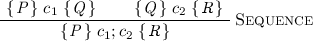
The rules for compound statements are slightly more complicated. To sequence two commands $c_{1}$ and $c_{2}$, the rule Seq requires the precondition of $c_{1}$ should hold and its postcondition should imply the postcondition of $c_{2}$. The postcondition of the composition states that there is an intermediate state $t$, that relates the postconditions of both statements.

The rule for conditionals, If, is reasonably straightforward: when the boolean condition $b$ holds, the precondition of the -branch must be satisfied and its postcondition is the postcondition of the entire statement. When the boolean condition is not satisfied, a similar statement holds for the -branch.

Finally, the While rule is the most complex. Besides the precondition, $P$, and postcondition, $Q$, associated with the body of the loop, the While rule requires the programmer to specify the loop invariant, $I$. The precondition of the While rule consists of three conjuncts:

• the invariant $I$ must hold initially;

• the boolean guard $b$ holds and the invariant must together imply the precondition of the loop body;

• the loop body must preserve the invariant.

The postcondition merely states that the boolean guard no longer holds, but the invariant has been maintained. Note that this formulation captures partial correctness; there is no variant ensuring that the loop must terminate eventually.

Using these semantics, we now define a refinement relation between statements in the While language:

Once again, we will use the notation $c_{1}\;\sqsubseteq \;c_{2}$ when $RefinedBy \;c_{1}\;c_{2}$ holds.

Example: Swap

With these definitions in place, we can now formalize the proof in Fig. 1. To do so, we need to find a proof of the $swapCorrect$ lemma, formulated as follows:

Here we use the $Ref$ constructor to include variables in our expression language. The proof is reasonably straightforward: we repeatedly apply the transitivity of the refinement relation, explicitly passing the mediating $Statement$ that we read off from Fig. 1. The only non-trivial proof obligations that arise concern reading from and writing to our heap.

Unfortunately, this form of post-hoc verification is very different from the program calculation that we would like to perform. The proof requires repeatedly stating the ‘next step’ in the refinement proof explicitly, every time we apply transitivity of the refinement relation. As a result, the straightforward proof script is lengthy and error-prone. In the next section we will develop machinery to enable the interactive discovery of programs, rather than the mere transcription of an existing proof.

5 Interactive Refinement

Although we can now take any pen-and-paper proof of refinement and verify this in Coq, we are not yet playing to the strengths of the interactive theorem prover that we have at hand. In this section, we will show how to develop lemmas and definitions on top of those we have seen so far that facilitate the interactive calculation of a program from its specification. Carefully choosing the formulation of our lemmas and the order of their assumptions will help guide the refinement process.

We start by defining a function that determines when a statement is executable, i.e., when there are no occurrences of the $Spec$ constructor:

Rather than fixing the exact program upfront, we can now reformulate the correctness lemma of swap as follows:

The notation $\{ x \mathbin {:} A \mid P \; x \}$ in Coq is used to denote a dependent pair consisting of a witness $x \mathbin {:} A$ and a proof that $x$ satisfies the property $P$.

To prove this lemma we need to provide an executable $c \mathbin {:} Statement$ and a proof that $SwapSpec \;\sqsubseteq \; c$. This is a superficial change – we could now complete the proof by providing our $swap$ program as the witness $c$ and reuse our previous correctness lemma. Instead of doing this, however, we wish to explore how to reformulate typical refinement calculus laws to enable the interactive construction of a suitable program.

Consider the following assignment rule, given in Lemma 2. We can formulate and prove the lemma in Coq as follows:

Here we use the notation $s' \;[ x \;\mapsto \;\llbracket e \rrbracket ]$ to indicate that the value associated with the identifier $x$ in $s'$ has been updated to $\llbracket e \rrbracket$. The proof of this lemma is reasonably straightforward. After applying the $Refinement$ constructor, the remaining proof obligations are trivial to discharge. Having proven this lemma, however, we cannot immediately use it to prove a goal of the shape $\{ c \mathbin {:} Statement \mid spec \;\sqsubseteq \; c \wedge isExecutable \; c \}$. To do so, we need to define an additional wrapper.

We can now use this lemma to finish our derivation, $swapCalc$. Every application of the $followAssign _2$ lemma changes the postcondition; once we have completed our three assignments, we will need to show that our postcondition is a direct consequence of our precondition. This last step is the most important and is the only step that requires any verification effort.

Looking at the formulation of the $followAssign _2$ lemma more closely, however, we see that we can always apply this rule, regardless of the pre- and postconditions of our specification. By heedlessly applying this lemma, we can paint ourselves into a corner, leaving an unprovable goal later on in the refinement derivation. Put differently, applying this rule defers all the verification work, whereas we would like to derive the overall correctness of a program from the correctness of a sequence of refinement steps.

To address this, we have defined the following final version of the following assignment rule:

Applying this rule yields two subgoals: the explicit proof relating the two postconditions and the remainder of the refinement calculation. Furthermore, when applying this rule the user must explicitly pass the ‘new’ postcondition $Q'$. This formulation of the following assignment rule, however, has one significant advantage: it encourages users to perform a small amount of verification, corresponding to the proof of first subgoal, every time it is applied. Where the previous formulations made it possible to rack up arbitrary ‘verification debt’, this last version enables the incremental development of the correctness proof.

This section has focused on a single lemma, $followAssign$. This lemma is representative for the design choices that we have made in the implementation of several related refinement laws. We have tried to capture our methodology in a handful of following design principles, that we applied when formulating further refinement laws:

• Any refinement law should prove a statement of the form $\{ c \mathbin {:} Statement \mid spec \;\sqsubseteq \; c \; \wedge \; isExecutable \; c \}$. Users are expected to formulate their specifications in this fashion. Fixing this form enables us to assume the open (sub)goals have a certain shape, which we can exploit during the program calculation and proof automation.

• There is at least one lemma implementing each of the refinement rules shown in Fig. 2. Often we provide several composite definitions, that refine specific parts of a composite command, such as the body of a loop or one component of a sequential composition.

• The order of hypotheses in lemmas matters. Coq presents the user with the remaining subgoals in the same order in which they occur as arguments to the lemma being invoked. Therefore subgoals that are most likely to be problematic should come first. For example, a poor choice of postcondition $Q'$ in the final version of the $followAssign$ lemma could yield unprovable subgoals. Requiring that problematic subgoals are completed first, minimizes the chance of a complete refinement calculation getting stuck on an unproven subgoal arising from an earlier step.

• We never assume anything about the shape of the pre- or postcondition of the specifications involved. For example, consider the usual rule for sequential composition from Hoare logic:

  

  To apply this rule, we require the precondition of $c_{1}$ and postcondition of $c_{2}$ to be identical. This is not necessarily the case in the middle of a refinement calculation. Instead of requiring users to weaken postconditions and strengthen preconditions explicitly, it can be useful to provide an equivalent, yet more readily applicable, alternative definition:

  

  Here we have turned the explicit relation between the postcondition of $c_{1}$ and the precondition of $c_{2}$ into an additional subgoal. As a result, the rule can always be applied, but it now carries an additional proof obligation.

6 Validation

This section presents two separate results, validating our work. We will show how our choice of pre- and postconditions associated with the While are sound and complete with respect to the usual weakest precondition semantics. Later, we will use our definitions to formalize a derivation by Morgan (1990).

Soundness

In Fig. 2, we are free to associate any choice of pre- and postconditions with the syntax of the While language – how can we validate that our choice of pre- and postconditions are correct? Or what does ‘correctness’ even mean in this context? In this section, we will show how our definitions relate to those found in the literature.

Typically, weakest precondition semantics are specified by associating predicate transformers with the constructs from a programming language. For example, the rules typically associated with the While language are give in Fig. 3.

Fig. 3.

Weakest precondition semantics of While

On the surface, the pre- and postconditions we have chosen in Fig. 2 are not at all similar. Yet we can relate these two semantics precisely. The semantics given in Fig. 3 define a function $\mathsf {wp}\!$ with the following type:

Recall from Sect. 3 that we can assign semantics to any value of $PT$, interpreting it as a predicate transformer of type $Pred \; S \rightarrow Pred \; S$. Using this semantics, we can now relate our definitions with the traditional semantics in terms of weakest preconditions:

This result is important: our choice of semantics in Fig. 2 is sound and complete with respect to the usual axiomatic semantics in terms of predicate transformers.

Case Study: Square Root

Now that we have covered the basic design principles and semantics of our embedding of the refinement calculus, we aim to validate our results through a case study. In this section, we will repeat the calculation of a program to performs a binary search to find the integer square root of its input integer. This example is taken from Morgan’s textbook on refinement calculus (Morgan 1990, Chap. 9). The complete calculation can be found in Fig. 4. Note that we have numbered every refinement step explicitly.

Fig. 4.

Calculating the integer square root program

Given the desired postcondition, , we apply several refinement laws until we are left with an executable program. To avoid repetition, we use the notation when the term contains a single specification that can be refined by . In particular, any executable code fragments in $P$ will not be repeated in (or the remainder of the derivation). This is a slight variation on the notation that Morgan uses, that more closely follows the intuition of ‘open subgoal’ with which users of interactive theorem provers will already be familiar.

The first step strengthens the postcondition, requiring that the additional condition must also be satisfied. In later steps, this will become our loop invariant, stating that our current approximation lies between the upper bound and lower bound . The proof continues by splitting off a series of assignments that ensure holds initially ().

Once we have established that the loop invariant holds initially (), we introduce a statement (). The loop will continue until the lower bound, , can no longer be increased without overlapping with the upper bound . Although we could refine the body of the with the command, this would cause our program to diverge. Instead, we begin by assigning to the variable the ‘halfway point’ between our bounds and (). Finally, we check whether is too large or too small to be the integer square root (). Both branches of the conditional update our bounds accordingly, after which the loop body is finished ().

How difficult is it to perform such a refinement proof in Coq? Most individual refinement steps correspond to a single call to an appropriate lemma. Discharging the subgoals arising from the application of each lemma typically requires a handful of tactics, many of which we believe could be automated further. The only non-obvious steps arise from having to apply several custom lemmas about division by two. The entire proof script weighs in at just under 200 lines, excluding general purpose lemmas defined elsewhere; as some of our lemmas require explicit pre- and postconditions, the proof scripts can become rather verbose. This is unfortunate, as adapting the specification may require updating the conditions mentioned explicitly in the proof script. We believe that it should be able to halve the length of the proof by tidying up the proof and investing in better automation.

Interactive verification in this style has several important advantages. Firstly, it is impossible to fudge your ‘proofs.’ On paper, it can be easy to gloss over certain verification conditions that you believe to hold. The proof assistant keeps you honest. Furthermore, the interactive derivation in this style produces an abstract syntax tree of the executable code. This can be easily traversed to generate imperative (pseudo)code. Some of the errors that Morgan describes arise from the fact that, even after the pen and paper proof has been completed, the resulting code still needs to be transcribed to a programming language. This need not be a concern in this setting.

7 Discussion

The choice of our $PT$ types and definition of refinement relation are not novel. Similar definitions of indexed containers (Altenkirch and Morris 2009) and interaction structures (Hancock and Setzer 2000a,b) can already be found in the literature. Indeed, part of this work was triggered by Peter Hancock’s remark that these structures are closely related to predicate transformers and the refinement relation between them, as we have made explicit in this paper.

We are certainly not the first to explore the possibility of embedding a refinement calculus in a proof assistant. One of the first attempts to do so, to the best of our knowledge, was by Back and Von Wright (Back and von Wright 1989). They describe a formalization of several notions, such as weakest precondition semantics and the refinement relation, in the interactive theorem prover HOL. This was later extended to the Refinement Calculator (Butler et al. 1997), that built a new GUI on top of HOL using Tcl/Tk. More recently, Dongol et al. have extended these ideas even further in HOL, adding a separation logic and its associated algebraic structure (Dongol et al. 2015). There are far fewer such implementations in Coq, Boulmé (2007) being one of the few exceptions. In contrast to the approach taken here, Boulmé explores the possibility of a monadic, shallow embedding, by defining the Dijkstra Specification Monad.

There is a great deal of work marrying effects and dependent types. Swierstra’s thesis explores one potential avenue: defining a functional semantics for effects (Swierstra 2009b; Swierstra and Altenkirch 2007). For some effects, such as non-termination, defining such a functional semantics in a total language is highly non-trivial. Therefore, systems such as Ynot take a different approach (Nanevski et al. 2008)s. Ynot extends Coq with several axioms, corresponding to the different operations various effects support, such as reading from and writing to mutable state. The type of these axioms captures all the information that a programmer may use to reason about such effects. These types are similar to those presented here in Fig. 2. Contrary to the approach taken here, however, Ynot lets users write their programs without considering their specification. Users only need to write proofs after specifying the pre- and postconditions for a certain function. The refinement calculus, on the other hand, starts from a specification, which is gradually refined to an executable program.

In the future, we hope to investigate how these various approaches to verification may be combined. One obvious next step would be to re-use the separation logic and associated proof automation defined by later installments of Ynot (Chlipala et al. 2009) as the model of the heap in our refinement calculus. Furthermore, we have (for now) chosen to ignore the variants associated with loops. As a result, the programs calculated may diverge. Embellishing our definitions with loop variants is straightforward, but will make our definitions even more cumbersome to use.

Type theory and the refinement calculus are both frameworks that combine specification and calculation. By embedding the refinement calculus in type theory, we study their relation further. The interactive structure of many proof assistants seems to fit well with the idea of calculating a program from its specification step-by-step. How well this approach scales, however, remains to be seen. For now, the embedding presented in this paper identifies an alternative point in the spectrum of available proof techniques for the construction of verified programs.

References

Altenkirch, T., Morris, P.: Indexed containers. In: 24th Annual IEEE Symposium on Logic in Computer Science, LICS 2009, pp. 227–285 (2009)
Back, R.J.R., von Wright, J.: Refinement concepts formalized in higher order logic. Formal Aspects Comput. 2, 247–272 (1989)
Von Wright, J.: Refinement Calculus: Refinement Calculus. Texts in Computer Science. Springer, New York (1998)
Back, R.J.R., von Wright, J.: Refinement concepts formalised in higher order logic. Formal Aspects Comput. 2(1), 247–272 (1990)
Back, R.J.R.: On the Correctness of Refinement in Program Development. PhD thesis, University of Helsinki (1978)
Boulmé, S.: Intuitionistic refinement calculus. In: Della Rocca, S.R. (ed.) TLCA 2007. LNCS, vol. 4583, pp. 54–69. Springer, Heidelberg (2007)
Butler, M.J., Grundy, J., Långbacka, T., Ruksenas, R., Wright, J.V.: The refinement calculator. In: Formal Methods Pacific (1997)
Chlipala, A., Malecha, G., Morrisett, G., Shinnar, A., Wisnesky, R.: Effective interactive proofs for higher-order imperative programs. In: International Conference on Functional Programming, ICFP 2009, pp. 79–90 (2009)
Dijkstra, E.W.: A Discipline of Programming. Prentice-Hall, Englewood Cliffs (1976)
Dongol, B., Gomes, V.B.F., Struth, G.: A program construction and verification tool for separation logic. In: Hinze, R., Voigtländer, J. (eds.) MPC 2015. LNCS, vol. 9129, pp. 137–158. Springer, Heidelberg (2015)
Floyd, R.W.: Assigning meanings to programs. Math. Aspects Comput. Sci 19(19–32), 1 (1967)
Hancock, P., Hyvernat, P.: Programming interfaces and basic topology. Ann. Pure Appl. Logic 137(1), 189–239 (2006)
Setzer, A., Hancock, P.: Interactive programs in dependent type theory. In: Clote, P.G., Schwichtenberg, H. (eds.) CSL 2000. lncs, vol. 1862, pp. 317–339. Springer, Heidelberg (2000)
Hancock, P., Setzer, A.: Specifying interactions with dependent types. In: Workshop on subtyping and dependent types in programming (2000b)
Hoare, C.A.R.: An axiomatic basis for computer programming. Commun. ACM 12(10), 576–580 (1969)
Morgan, C.: Programming from specifications. Prentice-Hall Inc, Upper Saddle River (1990)
Nanevski, A., Morrisett, G., Shinnar, A., Govereau, P., Birkedal, L.: Ynot: Dependent types for imperative programs. In: International Conference on Functional Programming, ICFP 2008, pp. 229–240 (2008)
Flemming, N., Nielson, H.R., Hankin, C.: Principles of Program Analysis. Springer, Heidelberg (1999)
Swierstra, W.: A hoare logic for the state monad. In: Berghofer, S., Nipkow, T., Urban, C., Wenzel, M. (eds.) TPHOLs 2009. LNCS, vol. 5674, pp. 440–451. Springer, Heidelberg (2009)
Swierstra, W.: A functional specification of effects. PhD thesis, University of Nottingham (2009)
Swierstra, W., Altenkirch, T.: Beauty in the beast: In: Proceedings of the ACM SIGPLAN Workshop on Haskell Workshop, pp. 25-36. ACM (2007)
Acknowledgments
The first author would like to thank Peter Hancock for his patience in explaining the relation between interaction structures and the refinement calculus. The first author’s visit to Scotland was funded by the London Mathematical Society’s Scheme 7 grant.
Author information
Authors and Affiliations
Corresponding author
Editor information
Editors and Affiliations
Rights and permissions
Copyright information
© 2016 Springer International Publishing Switzerland
About this paper
Cite this paper
Swierstra, W., Alpuim, J. (2016). From Proposition to Program. In: Kiselyov, O., King, A. (eds) Functional and Logic Programming. FLOPS 2016. Lecture Notes in Computer Science(), vol 9613. Springer, Cham. https://doi.org/10.1007/978-3-319-29604-3_3
Download citation
DOI: https://doi.org/10.1007/978-3-319-29604-3_3
Published:
Publisher Name: Springer, Cham
Print ISBN: 978-3-319-29603-6
Online ISBN: 978-3-319-29604-3
eBook Packages: Computer ScienceComputer Science (R0)