Explaining Graph Navigational Queries

Abstract

Graph navigational languages allow to specify pairs of nodes in a graph subject to the existence of paths satisfying a certain regular expression. Under this evaluation semantics, connectivity information in terms of intermediate nodes/edges that contributed to the answer is lost. The goal of this paper is to introduce the GeL language, which provides query evaluation semantics able to also capture connectivity information and output graphs. We show how this is useful to produce query explanations. We present efficient algorithms to produce explanations and discuss their complexity. GeL machineries are made available into existing SPARQL processors thanks to a translation from GeL queries into CONSTRUCT SPARQL queries. We outline examples of explanations obtained with a tool implementing our framework and report on an experimental evaluation that investigates the overhead of producing explanations.

Part of this work was done while G. Pirrò was working at the WeST institute, University of Koblenz-Landau supported by the FP7 SENSE4US project.

1 Introduction

Graph data pervade everyday’s life; social networks, biological networks, and Linked Open Data are just a few examples of its spread and flexibility. The limited support that relational query languages offer in terms of recursion stimulated the design of query languages where navigation is a first-class citizen. Regular Path Queries (RPQs) [6], and Nested Regular Expressions (NREs) [16] are some examples. Also SPARQL has been extended with a (limited) navigational core called property paths (PPs). As for query evaluation, the only tractable languages are 2RPQs and NREs; adding conjunction (C2RPQs) makes the problem intractable (NP-complete) while evaluation of PPs still glitches (mixing set and bag semantics). Usually, queries in all these languages ask for pairs of nodes connected by paths conforming to a regular language over binary relations.

We research the problem of enhancing navigational languages with explanation functionalities and introduce the Graph Explanation Language (GeL in short). In particular, our goal is to define formal semantics and efficient evaluation algorithms for navigational queries that return graphs useful to explain the results of a query.

GeL is useful in many contexts where one needs to connect the dots [11]; from bibliographic networks to query debugging [8]. The practical motivation emerged from the SENSE4US FP7 project¹ aiming at creating a toolkit to support information gathering, analysis and policy modeling. Here, explanations are useful to enable users to find out previously unknown information that is of relevance for a query, understand how it is of relevance, and navigate it. For instance, a GeL query on DBpedia and OpenEI using concepts like Country and Vehicle (extracted from a policy document) allows to retrieve, for instance, the pair (Germany, ElectricCar) and its explanation, which includes the company ThyssenKrupp (intermediate node). This allows to deduce that ThyssenKrupp is potentially affected by policies about electric cars.

GeL by Example. We now give an example of what GeL can express (the syntax and semantics are introduced in Sect. 3).

Example 1

(Co-authors). ISWC co-authors between 2002 and 2015.

The query uses path concatenation (/) nesting ([]), boolean combinations (${ \& \& }$) of (node) tests { } and backward navigation (^). The GeL syntax is purposely similar to previous navigational languages (e.g., NREs [16]). What makes a difference is the query evaluation semantics. Under the semantics of previous navigational languages, the evaluation would only look for pairs of co-authors (bindings of the variables ?x and ?y) connected by paths (in the graph) that satisfy the query. Under the GeL semantics, one can obtain both pairs of co-authors and a graph that gives an account of why each pair is an answer. Figure 1 shows the GUI of our explanation tool when evaluating the query on RDF data from DBLP. The tool allows to detail the explanation for each node in the answer. We only report explanations for $\texttt {?x}\rightarrow$ S. Staab in Fig. 1(a) and $\texttt {?x}\rightarrow$ C. utierrez in Fig. 1(b). One can see why S. Staab is linked with his co-authors; he had a paper with P. Mika, and R. Siebes and J. Brokestra are also authors of this paper. As for C. Gutierrez, we see that he had 8 ISWC papers, two of which with the same co-authors (i.e., M. Arenas and J. Pérez). $\blacktriangleleft$

Fig. 1.

ISWC co-authorship for S. Staab and C. Gutierrez.

Contributions and Outline. We contribute: (i) GeL, which to the best of our knowledge is the first graph navigational language able to produce (visual) query explanations; (ii) formal semantics; (iii) efficient algorithms; (iv) a GeL2CONSTRUCT translation, which makes our framework readily usable on existing SPARQL processors; (v) an evaluation that investigates the overhead of the new explanation-based semantics.

The remainder of the paper is organized as follows. Section 3 provides some background, presents the GeL language, formalizes the notion of graph query explanation and introduces the formal semantics of the language. Section 4 presents the evaluation algorithms, a study of their complexity and outlines the GeL2CONSTRUCT translation. We discuss an experimental evaluation in Sect. 5, sketch future work and conclude in Sect. 6.

2 Related Work

The core of graph query languages are Regular Path Queries (RPQs) that have been extended with other features, among which, conjunction (CRPQs) [6], inverse (C2RPQs) and the possibility to return and compare paths (EXPQs) [5]. Languages such as Nested Regular Expressions (NREs) [16] allow existential tests in the form of nesting, in a similar spirit to XPath. Finally, some languages have been proposed for querying RDF or Linked Data on the Web (e.g., [1, 2, 12, 13]). There are some drawbacks that hinder the usage of these languages for our goal. The evaluation of queries in these languages (apart from ERPQs) returns set of pairs of nodes or set of (solution) mappings and no connectivity information is kept. Query evaluation in most of these languages (including ERPQs that return graphs) is not tractable (combined complexity); those languages that are tractable (e.g., NREs, RPQs) do not output graphs. We design efficient algorithms to reconstruct parts of the graph traversed to build to the answer.

There are approaches to retrieve subgraphs, querying for semantic associations and/or providing relatedness explanations. As for the first strand, we mention $\rho$-Queries [4] and SPARQ2L [3]; here the idea is to enhance RDF query languages to deal with semantic associations or path variables and constraints. Our work is different since we focus on navigational queries and our algorithms for query evaluation under the graph semantics are polynomial. As for the second strand, we mention RECAP [17], RelFinder [14], Explass [7] that generate relatedness explanation when giving as input two entities and a maximum distance k. The idea is to generate SPARQL queries (typically 2$^k$ SPARQL queries) to retrieve paths of length k connecting the input pair; then, show paths after performing some filtering (e.g., only considering a subset of paths). The input of these approaches is a set of entities while in our case is a declarative navigational query; moreover, these approaches consider paths of a fixed length k (given as input) and require (SPARQL) queries to find these paths. Our work is also related to: (i) provenance (e.g., [9]); (ii) annotations (e.g., [22]) and (iii) module extraction (e.g., [19]).

Research in (i) and (ii) do not directly touch upon the problem of providing query explanations; their focus is on provenance and require complex machinery (e.g., annotation of data tuples using semirings). Our work defines formal query semantics to return graphs and obtain explanations via graph navigation and efficient reconstruction techniques. We focus on a precise class of queries that can be evaluated (also under the graph semantics) in polynomial time. The focus of (iii) is on the usage of Datalog to extract modules at ontological level while ours is on enhancing graph languages to return graphs. We also recall recent approaches dealing with recursion in SPARQL [18], where graphs (obtained via CONSTRUCT) are used to materialize data needed for the evaluation of the recursive SELECT query. Our focus is on the definition of formal semantics and efficient algorithms to enhance navigational languages to return graphs, and build explanations in an efficient way. Finally, to make our framework available on existing SPARQL processors we have devised a GEL2CONSTRUCT translation.

3 Building Query Explanations with GeL

We now provide some background information and then present the GeL language. We focus our attention on the Resource Description Framework (RDF). An RDF triple is a tuple of the form $\langle s,p,o \rangle \in \mathbf I \times \mathbf I \times \mathbf I \cup \mathbf L$, where $\mathbf I$ (IRIs) and $\mathbf L$ (literals) are countably infinite sets. Since we are interested in producing query explanations we do not consider bnodes. An RDF graph $G$ is a set of triples. The set of terms of a graph will be $terms(G)\subseteq \mathbf I \cup \mathbf L$; nodes(G) will be the set of terms used as a subject or object of a triple while triples(G) is the set of triples in G. Since SPARQL property paths offer very limited expressive power, we will consider the well-known Nested Regular Expressions (NREs) as reference language. NREs [16] allow to express existential tests along the nodes in a path via nesting (in the same spirit of XPath) while keeping the (combined) complexity of query evaluation tractable. Each NRE nexp over an alphabet of symbols $\varSigma$ defines a binary relation $\llbracket nexp \rrbracket ^G$ when evaluated over a graph G. The result of the evaluation of an NRE is a set of pairs of nodes. Other extensions (e.g., EPPs [10]) although adding expressive power to NREs (e.g., EPPs add path conjunction and path difference), all return pairs of nodes. This motivates the introduction of GeL, which tackles the problem of returning graphs from the evaluation of navigational queries that also help to explain query results.

3.1 Syntax of GeL

The syntax of GeL is defined by the following grammar:

$$ \begin{aligned} gexp :=&\tau \#exp\quad (\tau \in \{{\textsc {full}}, {\textsc {filtered}},set\}) \\ exp:=&a\ gtest(a\in \varSigma ) \mid ^a\ gtest(a\in \varSigma ) \mid exp \ / \ exp \mid exp\ | exp \mid exp^* \mid exp\{l,h\} \\ gtest:=&gtest \ \& \& \ gtest \mid gtest \ || \ gtest \mid (gtest) \mid [exp] \mid \{op \ val \} \\ op:=&> \ \mid \ < \ \mid \ =\ \mid \ \ne \end{aligned}$$

In the syntax, ^ denotes backward navigation, / path concatenation, | path union, {l,h} denotes repetition of an exp between l and h times;&& and || conjunction and disjunction of gtest, respectively. Moreover, when the gtest is missing after a predicate, it is assumed to be the constant true. We kept the syntax of the language similar to that of NREs and other languages. We define novel query semantics and evaluation algorithms capable of: (i) returning graphs; (ii) keeping query evaluation tractable; (iii) building query explanations. The syntactic construct $\tau$ allows to output the answer either in the form of pairs of nodes (i.e., set) as usually done by previous navigational languages or in the form of an explanation. GeL can produce two types of explanations: one keeping the whole portion of the graph “touched” during the evaluation (full) and the other keeping only paths leading to results (filtered).

3.2 Semantics of GeL

Tiddi et al. [21] define explanations as generalizations of some starting knowledge mapped to another knowledge under constraints of certain criteria. We use GeL queries to define starting knowledge and Explanation Graphs (EGs) to formally capture the criteria that knowledge included into an explanation has to satisfy.

Definition 2

(Explanation Graph). Given a graph G, a GeL expression e and a set of starting nodes $S\subseteq nodes(G)$, an EG is a quadruple $\varGamma$=(V, E, S, T) where $V\subseteq nodes(G)$, $E \subseteq triples(G)$ and $T\subseteq V$ is a set of ending nodes, that is, nodes reachable from nodes in S via paths satisfying e.

Fig. 2.

An example graph.

Consider the graph G in Fig. 2 and the expression e=(:knows/:knows)$\mid$(:co-author/:co-author). The answer with the semantics based on pairs of nodes (i.e., NREs) is the set of pairs of nodes: (a,c), (b,d). Under the GeL semantics, since there are two starting nodes a and b from which the evaluation produces results, one possibility would be to consider the EG capturing all results, that is, $\varGamma$=$(nodes(G), triple(G),\{\textit{a,c}\},\{\textit{b,d}\})$. However, one may note that there exists a path (via the node f) from $\textit{a}$ to $\textit{d}$ in the EG even if the pair $(\textit{a,d})$ does not belong to the answer. This could lead to misinterpretation of the query results and their explanation. To avoid these situations, we define G-soundness and G-completeness for EGs.

Definition 3

(G-Soundness). Given a graph G and a GeL expression e, an EG is G-sound iff each ending node is reachable in EG from each starting node via a path satisfying e.

Definition 4

(G-Completeness). Given a graph G and a GeL expression e, an EG is G-complete iff all nodes reachable from some starting nodes, via a path satisfying e, are in the ending nodes.

The EG $\varGamma$ in the above example violates G-soundness because there exists only one path (via the node $\textit{f}$) from $\textit{a}$ to $\textit{d}$ in $\varGamma$ and such path does not satisfy the expression e. The following lemma guarantees G-soundness and G-completeness.

Lemma 1

(G-Sound and G-Complete EGs). Explanation Graphs having a single starting node $v\in nodes(G)$ are G-sound and G-complete.

Definition 5

(Query Explanation). Given a GeL expression e and a graph G, a query explanation $\mathcal {E}^Q$ is a set of G-sound and G-complete EGs $\varGamma _v$.

Returning to our example, the query explanation is the set $\{\varGamma _a,\varGamma _b\}$ s.t.:

• 1. $\varGamma _a$=$(\{\textit{a,f,c}\},\{\langle \textit{a}, \texttt {:knows},\textit{f} \rangle ,\langle \textit{f},\texttt {:knows},\texttt {c} \rangle ,\textit{a},\{\textit{a,c}\})$

• 2. $\varGamma _b$=$(\{\textit{b,f,d}\},\{\langle \textit{b},\texttt {:co-author},\textit{f} \rangle ,\langle \textit{f},\texttt {:co-author},\textit{d} \rangle \},$ $\textit{b},\{\textit{b,d}\})$.

Note that query answering under the semantics returning pairs of nodes can be represented via the query explanation composed of the set of EGs: $\{\varGamma _v=(\emptyset ,\emptyset ,v,T)\mid v$ $\in$ $nodes(G)\}$. Since the formal semantics of GeL manipulates EGs, we now define: the counterpart for EGs of the composition () and union () operators used for binary relations, and operators to work with sets of EGs.

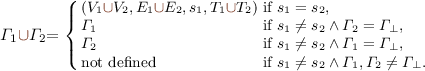
Definition 6

(EGs operators). Let $\varGamma _i = (V_i,E_i,s_i,T_i)$, $i=1,2$ be EGs and $\varGamma _{\perp }=(\emptyset ,\emptyset ,\perp ,\emptyset )$ denote the empty EG, where $\perp$ is a symbol not in the universe of nodes.

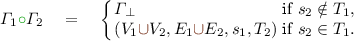
• Composition and union () of EGs:

  

  

The following definition formalizes extensions of the above operators over sets of EGs; here, the binary operator is applied to all pairs $\varGamma _1$, $\varGamma _2$ such that $\varGamma _1$ belongs to the first set and $\varGamma _2$ to the second one.

Definition 7

(Operations over sets of EGs). Let $S_1$ and $S_2$ be two sets of EGs.

• 1. For each op we define $S_1 \ \texttt {op} \ S_2 = \{ \varGamma _1 \texttt {op} \ \varGamma _2 \mid \varGamma _1\in S_1, \varGamma _2 \in S_2\}$.

• 2. (Disjoint union, direct sum): .

Table 1. The and semantics of GeL EGs. ($*$): rule valid for both. Repetitions of GeL expressions are translated into unions of concatenations. In lines 5, 6, 10 and 11 if gtest is not present then .

We now introduce the semantics of GeL in two variants: full () returning the portion of the graph visited during the evaluation and filtered (), which only considers successful paths. Let G be a graph and e a GeL expression. Under the semantics an explanation is the set of EGs where each EG $\varGamma _v$ includes the nodes and edges of G traversed during the evaluation of e from $v\in nodes(G)$. For this semantics we introduce, in Table 1, the evaluation function .

One may be only interested in the portion of G that actually contributed to build the answer; this gives the second semantics, where the query explanation is defined as the set of EGs such that each $\varGamma _v$ only considers paths that start from $v\in nodes(G)$ and satisfy the expression (i.e., the successful paths). We introduce the evaluation function in Table 1. The difference between the semantics lays in the sets of nodes (V) and edges (E) included in the explanations graphs that form a query explanation. An expression is evaluated either via the rule at line 1 or 2, depending on the type of semantics (explanation) wanted.

GeL expressiveness. We chose NREs as reference language and added the possibility to test for node values reached when evaluating a nested expression and boolean combinations of tests. We added this type of tests since they allow to express queries like those in Example 1. Nevertheless, the focus of this paper is on defining semantics and evaluation algorithms for navigational languages to output graphs besides pairs of nodes. This feature is not available in any existing navigational language (e.g., NREs [16], EPPs [10], SPARQL property paths).

4 Algorithms and Complexity

This section presents algorithms for the evaluation of GeL expressions under the novel semantics that also generate query explanations. The interesting result is that the evaluation of a GeL expression e in this new setting can be done efficiently. Let e be a GeL expression and G a graph. Let |e| be the size of e, $\varSigma _e$ the set of edge labels appearing in it, and |G|=$|nodes(G)|+|triples(G)|$ be the size of G. Algorithms that build explanations according to the full or filtered semantics are automata-based and work in two steps. The first step is shared and leverages product automata; the second step requires a marking phase only for the filtered semantics and is needed to include nodes and edges in the EGs that are relevant for the answer.

Building Product Automata. The idea is to associate to e (and to each gtest on the form of [exp]) a non deterministic finite state automaton with $\epsilon$ transitions $\mathcal {A}_{e}$ ($\mathcal {A}^{exp}$, resp.). Such automata can be built according to the standard Thomson construction rules over the alphabet Voc(e)=$\varSigma _e\cup \bigcup _{gtest\in e} gtest$, that is, by considering also gtest in e as basic symbols. The product automaton is a tuple $G\times \mathcal {A}_e=\langle Q^e,Voc(e),\delta ^e,Q^e_0,F^e\rangle$ where $Q^e$ is a set of states, $\delta ^e$:$Q^e\times (Voc(e)\cup \epsilon ) \rightarrow 2^{Q^e}$ is the transition function, $Q^e_0\subseteq Q^e$ is the set of initial states, and $F^e\subseteq Q^e$ is the set of final states. The building of the product automaton $G\times \mathcal {A}_e$ is based on an extension of the algorithm used by [16] based on the labeling of the nodes of G. In this phase, G is labeled wrt nested subexpressions in e, that is, for each node $n \in nodes(G)$ and nested subexpression exp in e, $exp \in label(n)$ if and only if there exists a node $n'$ such that there is a path from n to $n'$ in G satisfying exp. This allows to recursively label the graph G for each [exp]; hence, when the labeling wrt exp has to be computed, G has already been labeled wrt all the nested subexpressions $[exp']$ in exp.

Theorem 8

([16]). The product $G\times \mathcal {A}_{e}$ can be built in time $O(|G| \times |e|)$.

Building Explanations. We now discuss algorithms that leverage product automata (of the GeL expression e and all nested subexpressions) to produce graph query explanations according to the full and filtered semantics. To access the elements of an explanation graph $\varGamma$ (see Definition 2) we use the notation $\varGamma .x$, with $x\in \{V,E,S,T\}$. The main algorithm is Algorithm 1, which receives the GeL expression and the type of explanation to be built. In case of the filtered semantics the data structure reached, which maintains a set of states $(n_i,q_j)$, is initialized via the procedure mark (line 3) reported in Algorithm 2; otherwise, it is initialized as the union of: (i) all the states of the product automaton $G\times \mathcal {A}_e$; (ii) all the states of the product automata ($G\times \mathcal {A}_{exp}$) of all the nested expressions in e (line 5). The procedure mark fills the set reached with all the states in all the product automata that contribute to obtain an answer; these are the states in a path from an initial state to a final state in the product automata. As shown in Algorithm 2, reached is populated by navigating the product automata backward from the final states to the initial ones. Then, the set of EGs composing a query explanation $\mathcal {E}^Q$ are initialized (lines 6–7; 9) by adding to $\mathcal {E}^Q$ an EG $\varGamma _s$ for each initial state $(s,q_0)$ of $G\times \mathcal {A}_e$. Moreover, the data structure seen is also initialized (line 8) by associating to each state $(s,q_0)$ the node s (associated to the initial state $(s,q_0)$) from which it has been visited.

The data structure seen maintains for each state, reached while visiting the product automata, the starting nodes from which this state has already been visited. The usage of seen avoids to visit the same state more than once for each starting node. Finally, the data structure visit is also initialized with the initial states of $G\times \mathcal {A}_e$ (line 10); it contains all the states to be visited in the subsequent step plus the set of starting nodes for which these states have to be visited. Then, the EGs are built via buildE (Algorithm 3); all the states in visit are considered (line 2) only once for the entire set $B_{n,q}$, which keeps starting nodes for which states in visit have to be processed (line 3). Then, for each state $(n,q) \in$ visit all its transitions are considered (line 7); for each state $(n',q') \in$ reached, reachable from some $(n,q)\in visit$ via some transitions (line 8), the set of “new” starting nodes (D) for which $(n',q')$ has to be visited in the subsequent step is computed with a possible update of the sets visit and seen (lines 9–12). If the transition is labeled with a predicate symbol in G (line 13), the EGs corresponding to nodes $s\in B_{n,q}$ are constructed by adding the corresponding nodes and edges (lines 14–16). If the transition is a gtest the building of the query explanation $\mathcal {E}^Q$ proceeds recursively by visiting the product automata associated to all nested (sub)expressions for gtest (lines 17–21).

Theorem 9

Given a graph G and a GeL expression e, the query explanation $\mathcal {E}^Q$ (according to both semantics) can be computed in time $\mathcal {O}(|nodes(G)|\times |G|\times |e|)$.

Proof

The explanation $\mathcal {E}^Q$ built according to the full semantics can be constructed by visiting $G$ $\times$ $\mathcal {A}_e$ (Algorithm 3). In particular, for each starting state (n, q), the states and transitions of $G$ $\times$ $\mathcal {A}_e$ are all visited at most once (and the same also holds for the automata corresponding to the nested expressions of e). The starting and ending nodes of each EG are set during the visit of the product automaton. For each node s corresponding to a starting state $(s,q_o) \in Q^e_0$ an explanation graph $\varGamma _s$ is created (Algorithm 1, lines 6–7); the set of nodes reachable from s is set to be $\varGamma _s.T=\{\texttt {n}\mid (\texttt {n},q)\in F^e \text{ and } (n,q) \text{ is } \text{ reachable } \text{ from } (s,q_o)\}$ (Algorithm 3 lines 5–6). Thus, each EG can be computed by visiting each transition and each node exactly once with a cost $O(|Q^e|+\sum _{[exp]\in e} |Q^{exp}|+|\delta ^e|+\sum _{[exp]\in e} |\delta ^{exp}|)=O(|G|\times |e|)$. Since the number of EGs to be constructed is bound by |nodes(G)|, the total cost of building the query explanation $\mathcal {E}^Q$, is $\mathcal {O}(|nodes(G)|\times |G|\times |e|)$. This bounds also take into account the cost of building product automata as per Theorem 8.

In the case of the filtered semantics, the marking phase does not increase the complexity bound; this is because the set reachable, which keeps reachable states, is built by visiting at most once all nodes and transitions in all the product automata, with a cost $O(|G|\times |e|)$.    $\square$

Note that in Algorithm 3, the amortized processing time per node is lower than $|G|\times |e|$ when visiting the product automaton since the Breadth First Search(es) from each starting state are concurrently run according to the algorithm in [20]. Finally, the EGs in the $\mathcal {E}^Q$ built via Algorithm 1 are both G-sound and G-complete. It is easy to see by the definition of the product automaton, that there exists a starting state $(n,q_0)$ that is connected to a final state $(n',q_f)$ in $G\times \mathcal {A}_e$ and, thus, a path from n to $n'$ in $\varGamma _n$ if, and only if, there exists a path connecting n to $n'$ in G satisfying e.

4.1 Translating GeL into SPARQL

The algorithms discussed in Sect. 4 are suitable for the implementation of GeL on a custom query processor. This has the advantage to guarantee a low complexity of query evaluation as we have formally proved. On the other hand, there is SPARQL, which is the standard for querying RDF data although offering limited navigational capabilities (via property paths). We wondered how the machineries developed for GeL could be made available on existing SPARQL processors. This will have the advantage of making GeL readily available for usage on the tremendous amount of RDF data accessible through SPARQL endpoints. We have devised a formal translation (GEL2CONSTRUCT) from GeL queries into CONSTRUCT SPARQL queries that produce RDF graphs as results of a SPARQL query. In particular, since current SPARQL processors can handle limited forms of recursive queries (as studied by Fionda et al. [10]) only a subset of GeL queries can actually be turned into CONSTRUCT queries. Such queries do not include closure operators (i.e., *). We have included in GeL path repetitions, that is, the possibility to express in a succinct way the union of concatenations of a GeL expression between l and h times. When translating GeL into CONSTRUCT queries one has to give up two main things. First, the complexity of query evaluation increases even if one can now rely on efficient and mature SPARQL query processors. Second, it is possible to only produce explanations under the filtered semantics as SPARQL processors only provide parts of the graph that contribute to the answer while GeL relies on automata-based algorithms to also keep parts touched that do not contribute to the answer. Table 2 gives an overview of the translation. The translation algorithm, starts from the root of the parse tree of a GeL expression and applies translation rules recursively. Each GeL syntactic construct has associated a chuck of SPARQL code.

Table 2. Translating GeL into SPARQL (CONSTRUCT).

Theorem 10

For every (non-recursive) GeL query , $\alpha ,\beta \in \mathcal {V}\cup \mathbf I$, there exists a CONSTRUCT query $Q_e$=$\mathcal {A}^t(\mathcal {P})$ such that for every RDF graph $G$ it holds that $[\![\mathcal {P}]\!]_{G}$=$[\![{ Q_e}]\!]_{G}$. The GEL2CONSTRUCT algorithm $\mathcal {A}^t$ runs in time O($|\mathcal {P}|$).

Proof

(Sketch). The proof works by checking that the propagation of variable names (artificially generate) and terms along the parse tree is correct (see e.g., [10]).    $\square$

5 Implementation and Evaluation

We implemented GeL and the explanation framework in Java. Beside our custom evaluator based on the algorithms discussed in Sect. 4, we have also implemented the GEL2CONSTRUCT translation to make available GeL’s capabilities into existing SPARQL engines in an elegant and non-intrusive way.

Experimental Setting. We tested our approach using different datasets. The first is a subset of the FOAF network ($\sim$4M triples) obtained by crawling from 10 different seeds foaf:knows predicates up to distance 6 and then merging the graphs. The second one, is the Linked Movie Database (LMDB)², an RDF dataset containing information about movies and actors ($\sim$6M triples). We also considered data from YAGO (via the LOD cache³) ($\sim$22B triples) and DBpedia⁴ ($\sim$412M triples). The goal of the evaluation is to measure the overhead of outputting graphs as a result of navigational queries and build query explanations. Because of the novelty of our approach it was not possible to compare it against other implementations, or run standard benchmarks to test the overhead of outputting graphs instead of pairs of nodes. We tested the overhead of producing explanations both when using our custom processors and on SPARQL endpoints and also measured the size of the output returned. We used 6 queries per dataset for a total of 24 queries plus their SPARQL translation. Experiments have been run on a PC i5 CPU 2.6 GHz and 8 GB RAM; results are the average of 5 runs.

Overhead using the custom processor. We considered 6 queries (on FOAF data) including concatenations and gtest that ask for (pairs of) friends at increasing distance (from 1 to 6) with the condition that each friend (in the path) must have a link to his/her home page. For sake of space we report the overhead of generating explanations about Tim Berners-Lee (TBL) along with the size of the explanation (#nodes,#edges) generated under the filtered and full semantics (Tables 3 and 4). We observed a similar behavior when considering explanations related to other people in the FOAF network (e.g., A. Polleres, N. Lopes).

Table 3. Overhead (secs).

Table 4. Size of the explanation.

The evaluation of GeL queries under the explanation semantics does not have a significant impact on query processing time (the overhead is max. $\sim$2 s) for friends at distance 6. This is not surprising as it confirms the complexity analysis discussed in Sect. 4 where we showed that our explanations algorithms run in polynomial time. The output of a GeL query clearly requires more space as it is a (explanation) graph. As one may expect, the full semantics produces larger graphs than the filtered semantics as it reports all parts of the graph touched (i.e., even paths that did not lead to any result). We can observe that for TBL, at distance 6 the explanation contains 190 nodes and 139 edges (resp., 177 and 111) under the full semantics (resp., filtered). The visual interface of the tool implementing GeL (see Fig. 1) allows to picking one node in the output and generate the corresponding explanation graph, zoom the graph, change the size of nodes/edges and perform free text search for nodes/edges. Running time for all queries were in the order of 6 seconds. Note that our algorithms work with the graphs loaded into main memory. In the next experiment we measure the overhead of generating explanations on large set of triples.

Overhead on SPARQL endpoints. Since we made available GeL’s machinery also via CONSTRUCT queries, we tested the overhead of generating explanation (graphs) also on different datasets and SPARQL endpoints both local and remote. We set up a local BlazeGraph⁵ instance where we loaded LMDB and accessed the other datasets via their endpoints. For each dataset we created 6 GeL queries and translated them into: (i) SELECT queries to mimic the semantics returning pairs of nodes and (ii) CONSTRUCT queries to mimic the explanation semantics. At this point, we need to make two important observations about generating explanations via translation into SPARQL. First, it is only possible to consider the filtered semantics as SPARQL engines do not keep track of the portions of the graph visited that did not contribute to the answer necessary for the full semantics. Second, explanations are only G-complete (see Definition 5) as it is not possible to keep separate the explanation for each node in the result of a CONSTRUCT while it can be done in GeL by using Explanation Graphs (see Definition 2). The overhead and size of results for DBpedia and YAGO are reported in the following figures.

Fig. 3.

DBpedia Time.

Fig. 4.

DBpedia Size.

Fig. 5.

YAGO Time.

Fig. 6.

YAGO size.

As it can be observed, running time for the CONSTRUCT (explanation) queries are always higher in DBpedia (Fig. 3) but always $\sim$1 s. The size of results (# triples) (Fig. 4) reaches 800 for Q1, which asks for (all pairs) fo people that have influenced each other (no filters). From Q2–Q6 each person in an influence path must be a scientist; this filter decreases at each step the size of the answer ($\sim$100 for Q6). For YAGO (Fig. 5), accessed via LOD cache, we also observe that CONSTRUCT queries (asking for influences in YAGO among female people) require more time (<3 s) than SELECT queries, with an overhead of $\sim$2 s. Even in this case the overhead of generating explanations (considering the larger number of results generated) is bearable (Fig. 6). On LDMB (results not reported for sake of space) the overhead was of $\sim$1.5 s with average size of the explanation $\sim$700 triples. The GEL2CONSTRUCT translation (integrated in our tool) allows to obtain explanations from a variety of SPARQL endpoints online.

6 Concluding Remarks and Future Work

We have shown how current navigational languages (e.g., NREs) can be enhanced to return graphs besides pairs of nodes. Such kind of information is useful whenever one needs to connect the dots (e.g., bibliographic networks, exploratory search). We have described a language, formalized two semantics, and provided algorithms that use connectivity information to produce different types of query explanations. The interesting aspect is that query answering under the new explanation semantics is still tractable. We gave some examples of (visual) explanations generated with a tool implementing our framework and using real world data. There are several avenues for future research, among which: (i) studying explanations with negative information (e.g., which parts of a query failed); (ii) studying the expressiveness of GeL; (iii) assisting the user in writing queries [15]; (iv) including RDFS inferences.

References

Acosta, M., Vidal, M.-E.: Networks of linked data eddies: an adaptive web query processing engine for RDF data. In: Arenas, M., Corcho, O., Simperl, E., Strohmaier, M., d’Aquin, M., Srinivas, K., Groth, P., Dumontier, M., Heflin, J., Thirunarayan, K., Staab, S. (eds.) ISWC 2015. LNCS, vol. 9366, pp. 111–127. Springer, Cham (2015). doi:10.1007/978-3-319-25007-6_7
Alkhateeb, F., Baget, J.-F., Euzenat, J.: Extending SPARQL with regular expression patterns (for querying RDF). J. Web Sem. 7(2), 57–73 (2009)
Anyanwu, K., Maduko, A., Sheth, A.: SPARQ2L: towards support for subgraph extraction queries in RDF databases. In: WWW, pp. 797–806. ACM (2007)
Anyanwu, K., Sheth, A.: p-Queries: enabling querying for semantic associations on the semantic web. In: WWW, pp. 690–699. ACM (2003)
Barceló, P., Libkin, L., Lin, A.W., Wood, P.T.: Expressive languages for path queries over graph-structured data. ACM TODS 37(4), 31 (2012)
Calvanese, D., De Giacomo, G., Lenzerini, M., Vardi, M.Y.: Containment of conjunctive regular path queries with inverse. In: KR, pp. 176–185 (2000)
Cheng, G., Zhang, Y., Explass, Y.: Exploring associations between entities via top-k ontological patterns and facets. In: Proceedings of ISWC, pp. 422–437 (2014)
Consens, M.P., Liu, J.W.S., Rizzolo, F.: Xplainer: visual explanations of XPath queries. In: ICDE, pp. 636–645. IEEE (2007)
Dividino, R., Sizov, S., Staab, S., Schueler, B.: Querying for provenance, trust, uncertainty and other meta knowledge in RDF. J. Web Semant. 7(3), 204–219 (2009)
Fionda, V., Pirrò, G., Consens, M.P., Paths, E.P.: Writing more SPARQL queries in a succinct way. In: AAAI (2015)
Fionda, V., Gutierrez, C., Pirrò, G.: Building knowledge maps of web graphs. Artif. Intell. 239, 143–167 (2016)
Fionda, V., Pirrò, G., Gutierrez, C.: NautiLOD: a formal language for the web of data graph. ACM Trans. Web 9(1), 5:1–5:43 (2015)
Hartig, O., Pérez, J.: LDQL: a query language for the web of linked data. In: Arenas, M., Corcho, O., Simperl, E., Strohmaier, M., d’Aquin, M., Srinivas, K., Groth, P., Dumontier, M., Heflin, J., Thirunarayan, K., Staab, S. (eds.) ISWC 2015. LNCS, vol. 9366, pp. 73–91. Springer, Cham (2015). doi:10.1007/978-3-319-25007-6_5
Heim, P., Hellmann, S., Lehmann, J., Lohmann, S., Stegemann, T.: RelFinder: revealing relationships in RDF knowledge bases. In: Semantic Multimedia, pp. 182–187 (2009)
Lehmann, J., Bühmann, L.: AutoSPARQL: let users query your knowledge base. In: Antoniou, G., Grobelnik, M., Simperl, E., Parsia, B., Plexousakis, D., Leenheer, P., Pan, J. (eds.) ESWC 2011. LNCS, vol. 6643, pp. 63–79. Springer, Heidelberg (2011). doi:10.1007/978-3-642-21034-1_5
Pérez, J., Arenas, M., Gutierrez, C.: nSPARQL: a navigational language for RDF. J. Web Semant. 8(4), 255–270 (2010)
Pirrò, G.: Explaining and suggesting relatedness in knowledge graphs. In: Arenas, M., Corcho, O., Simperl, E., Strohmaier, M., d’Aquin, M., Srinivas, K., Groth, P., Dumontier, M., Heflin, J., Thirunarayan, K., Staab, S. (eds.) ISWC 2015. LNCS, vol. 9366, pp. 622–639. Springer, Cham (2015). doi:10.1007/978-3-319-25007-6_36
Reutter, J.L., Soto, A., Vrgoč, D.: Recursion in SPARQL. In: Arenas, M., Corcho, O., Simperl, E., Strohmaier, M., d’Aquin, M., Srinivas, K., Groth, P., Dumontier, M., Heflin, J., Thirunarayan, K., Staab, S. (eds.) ISWC 2015. LNCS, vol. 9366, pp. 19–35. Springer, Cham (2015). doi:10.1007/978-3-319-25007-6_2
Rousset, M.-C., Ulliana, F.: Extracting bounded-level modules from deductive RDF triplestores. In: Proceedings of the AAAI (2015)
Then, M., Kaufmann, M., Chirigati, F., Hoang-Vu, T., Pham, K., Kemper, A., Neumann, T., Vo, H.T.: The more the merrier: efficient multi-source graph traversal. VLDB Endowment 8(4), 449–460 (2014)
Tiddi, I., d’Aquin, M., Motta, E.: An ontology design pattern to define explanations. In: K-CAP, p. 3 (2015)
Zimmermann, A., Lopes, N., Polleres, A., Straccia, U.: A feneral framework for representing, reasoning and querying with annotated semantic web data. J. Web Semant. 11, 72–95 (2012)
Author information
Authors and Affiliations
Corresponding author
Editor information
Editors and Affiliations
Rights and permissions
Copyright information
© 2017 Springer International Publishing AG
About this paper
Cite this paper
Fionda, V., Pirrò, G. (2017). Explaining Graph Navigational Queries. In: Blomqvist, E., Maynard, D., Gangemi, A., Hoekstra, R., Hitzler, P., Hartig, O. (eds) The Semantic Web. ESWC 2017. Lecture Notes in Computer Science(), vol 10249. Springer, Cham. https://doi.org/10.1007/978-3-319-58068-5_2
Download citation
DOI: https://doi.org/10.1007/978-3-319-58068-5_2
Published:
Publisher Name: Springer, Cham
Print ISBN: 978-3-319-58067-8
Online ISBN: 978-3-319-58068-5
eBook Packages: Computer ScienceComputer Science (R0)