Conditional Disclosure of Secrets: Amplification, Closure, Amortization, Lower-Bounds, and Separations

Abstract

In the conditional disclosure of secrets problem (Gertner et al. J. Comput. Syst. Sci. 2000) Alice and Bob, who hold inputs x and y respectively, wish to release a common secret s to Carol (who knows both x and y) if and only if the input (x, y) satisfies some predefined predicate f. Alice and Bob are allowed to send a single message to Carol which may depend on their inputs and some joint randomness and the goal is to minimize the communication complexity while providing information-theoretic security.

Following Gay et al. (Crypto 2015), we study the communication complexity of CDS protocols and derive the following positive and negative results.

• (Closure): A CDS for f can be turned into a CDS for its complement $\bar{f}$ with only a minor blow-up in complexity. More generally, for a (possibly non-monotone) predicate h, we obtain a CDS for $h(f_1,\ldots ,f_m)$ whose cost is essentially linear in the formula size of h and polynomial in the CDS complexity of $f_i$.

• (Amplification): It is possible to reduce the privacy and correctness error of a CDS from constant to $2^{-k}$ with a multiplicative overhead of O(k). Moreover, this overhead can be amortized over k-bit secrets.

• (Amortization): Every predicate f over n-bit inputs admits a CDS for multi-bit secrets whose amortized communication complexity per secret bit grows linearly with the input length n for sufficiently long secrets. In contrast, the best known upper-bound for single-bit secrets is exponential in n.

• (Lower-bounds): There exists a (non-explicit) predicate f over n-bit inputs for which any perfect (single-bit) CDS requires communication of at least $\varOmega (n)$. This is an exponential improvement over the previously known $\varOmega (\log n)$ lower-bound.

• (Separations): There exists an (explicit) predicate whose CDS complexity is exponentially smaller than its randomized communication complexity. This matches a lower-bound of Gay et al., and, combined with another result of theirs, yields an exponential separation between the communication complexity of linear CDS and non-linear CDS. This is the first provable gap between the communication complexity of linear CDS (which captures most known protocols) and non-linear CDS.

1 Introduction

Consider a pair of computationally-unbounded parties, Alice and Bob, each holding an n-bit input, x and y respectively, to some public predicate $f:\{0,1\}^n\times \{0,1\}^n\rightarrow \{0,1\}$. Alice and Bob also hold a joint secret $s\in \{0,1\}$ and have access to a joint source of randomness $r\mathop {\leftarrow }\limits ^{R}\{0,1\}^{\rho }$. The parties wish to disclose the secret s to a third party, Carol, if and only if the predicate f(x, y) evaluates to 1. To this end, Alice (resp., Bob) should send to Carol a single message $a=a(x,s;r)$ (resp., $b=b(y,s;r)$). Based on the transcript (a, b) and the inputs (x, y), Carol should be able to recover the secret s if and only if $f(x,y)=1$. (Note that Carol is assumed to know x and y.) That is, we require two properties:

• Correctness: There exists a decoder algorithm $\mathsf {Dec}$ that recovers s from (x, y, a, b) with high probability whenever (x, y) is a 1-input (i.e., $f(x,y)=1$);

• Privacy: There exists a simulator $\mathsf {Sim}$ that, given a 0-input (x, y) (for which the predicate evaluates to 0), samples the joint distribution of the transcript (x, y, a, b) up to some small deviation error.

The main goal is to minimize the communication complexity of the protocol which is taken to be the total bit-length of the messages a and b. (See Sect. 3 for formal definitions.)

This form of Conditional Disclosure of Secrets (CDS) was introduced by Gertner et al. [18] as a tool for adding data privacy to information-theoretically private information retrieval (PIR) protocols [14] and was later used in the computational setting as a light-weight alternative to zero-knowledge proofs (cf. [2]). Apart from these applications, CDS plays a central role in the design of secret sharing schemes for graph-based access structures (cf. [10, 11, 37]) and in the context of attribute-based encryption [21, 35]. In fact, CDS can be equivalently formulated under any of these frameworks as discussed below.

Secret Sharing for Forbidden Graphs. CDS can also be viewed as a special form of secret sharing for graph-based access structures (cf. [10, 11, 37]). Specifically, consider a secret-sharing scheme whose parties are the nodes of a bipartite graph $G=(X\cup Y,E)$ and a pair of parties $(x,y)\in X\times Y$ should be able to recover the secret s if and only if they are connected by an edge. (It is also required that singletons are not authorized, but other than that we do not require any privacy/correctness condition for other subsets of parties). Then, we can represent the secret-sharing problem as the problem of realizing a CDS for the predicate $f_G(x,y)=1 \Leftrightarrow (x,y)\in E$ and vice-versa by setting the share of the x-th node (resp., y-th node) to be the message a(x, s; r) (resp., b(y, s; r)). The communication complexity of the CDS protocol therefore corresponds to the size of shares.

Attribute-Based Encryption. CDS can be further viewed as a limited form of private-key attribute-based encryption [21, 35] which offers one-time information-theoretic security. In such an encryption scheme both the decryption key $a_x$ of a receiver and the ciphertext $b_y$ of a sender are associated with some public attributes x and y, respectively. The receiver should be able to decrypt the plaintext m from the ciphertext $b_y$ using the key $a_x$ only if the attributes x and y “match” according to some predefined policy, i.e., satisfy some predicate f(x, y). Using CDS for f, we can derive such a one-time secure scheme by letting the decryption key be Alice’s message, $a_x=a(x,s;r)$, for a random secret s, and taking the ciphertext to be Bob’s message $b_y=b(y,s;r)$ together with a padded-version of the message $m\oplus s$. (Here we can think of (r, s) as the sender’s private-key.) In fact, it was shown by Attrapadung [8] and Wee [38] that even in the computational setting of public-key (multi-user) attribute-based encryption (ABE), linear CDS schemes (in which the computation of Alice and Bob can be written as a linear function in the secret an the randomness) form a central ingredient. As a result, the ciphertext size and secret key of the ABE directly depend on the communication complexity of the underlying CDS.

The Communication Complexity of CDS. In light of the above, it is interesting to understand the communication complexity of CDS. Unfortunately, not much is known. Gertner et al. [18] showed that any predicate f that can be computed by a s-size Boolean formula admits a perfect linear CDS (with zero correctness/privacy error) with communication complexity of O(s). This result was extended by Ishai and Wee [26] to s-size (arithmetic) branching programs and by Applebaum and Raykov [7] to s-size (arithmetic) span programs (though in the latter case correctness is imperfect). Beimel et al. [9] proved that the CDS complexity of the worst predicate $f:\{0,1\}^n\times \{0,1\}^n\rightarrow \{0,1\}$ over n-bit inputs is at most $O(2^{n/2})$. A similar upper-bound was later established by Gay et al. [17] for the case of linear CDS, where a matching (non-explicit) lower-bound follows from the work of Mintz [31]. Very recently, Liu et al. [29] improved the worst-case complexity of (non-linear) CDS to $2^{O(\sqrt{n \log n})}$. Gay et al. [17] also initiated a systematic treatment of the communication complexity of CDS and established the first lower-bounds on the communication complexity of general CDS. Their main result relates the CDS communication of a predicate f to its randomized communication complexity. Roughly speaking, it is shown that a general CDS for f must communicate at least $\varOmega (\log ( (\mathsf {R} (f)))$ bits, and a linear CDS must communicate at least $\varOmega (\sqrt{\mathsf {R} (f)})$, where $\mathsf {R} (f)$ denotes the number of bits communicated in a randomized protocol that need to be exchanged between Alice and Bob in order to compute f with constant error probability.¹ This yields (explicit) lower-bounds of $\varOmega (\log (n))$ and $\varOmega (\sqrt{n})$, respectively, for concrete n-bit predicates. Overall, for general CDS, there is an almost double-exponential gap between the best known (logarithmic) lower-bound and the best known ($2^{O(\sqrt{n \log n})}$) upper bound.

2 Our Results

Following Gay et al. [17], we conduct a systematic study of the complexity of CDS. Unlike previous works, we focus on manipulations and transformations of various forms of CDS. Our approach yields several positive and negative results regarding the complexity of CDS, and answers several open problems posed in previous works. We proceed with a statement of our results.

2.1 Closure Properties

We begin by asking whether one can generally combine CDS for basic predicates $f_1,\ldots ,f_m$ into a CDS for a more complicated predicate $h(f_1,\ldots ,f_m)$. Using standard secret sharing techniques, one can derive such a transformation when h is a monotone function (with overhead proportional to the monotone formula size of h). However, these techniques fail to support non-monotone operations. Our first observation asserts that linear CDS for f can be easily transformed into a linear CDS for its complement $\overline{f}\equiv 1-f$. (A similar observation was recently made by Ambrona et al. [4] in the related context of “linear predicate encodings”.²)

Theorem 1

(Linear CDS is closed under complement). Suppose that f has a linear $\mathsf {CDS}$ with randomness complexity of $\rho$ and communication complexity of t, then $\overline{f}$ has a linear $\mathsf {CDS}$ scheme with randomness complexity of $t+\rho +1$ and communication complexity of $2(\rho +1)$.

The theorem generalizes to arbitrary finite field $\mathbb {F}$. (See Sect. 4.1.) Roughly speaking, we rely on the following observation. It can be shown that, for a fixed input (x, y), the parties jointly compute some linear operator $T_{x,y}$ that has a high rank whenever $f(x,y)=0$, and low rank when $f(x,y)=1$. We “reverse” the CDS by essentially moving to the dual $T^*_{x,y}$ of $T_{x,y}$ whose rank is high when $f(x,y)=1$, and low when $f(x,y)=0$. One still has to find a way to distributively compute the mapping $T^*_{x,y}$. We solve this technicality by using a private simultaneous message protocol (PSM) [15] that allows Alice and Bob to securely release an image of $T^*_{x,y}$ to Carol without leaking any additional information.

Next, we show that a similar “reversing transformation” exists for general (non-linear and imperfect) CDS protocols.

Theorem 2

(CDS is closed under complement). Suppose that f has a $\mathsf {CDS}$ with randomness complexity of $\rho$ and communication complexity of t and privacy/correctness errors of $2^{-k}$. Then $\overline{f}\equiv 1-f$ has a $\mathsf {CDS}$ scheme with similar privacy/correctness errors and randomness/communication complexity of $O(k^3\rho ^2t+k^3\rho ^3)$.

Imitating the argument used for the case of linear CDS, we consider, for an input (x, y) and secret s, the probability distribution $D^s_{x,y}$ of the messages (a, b) induced by the choice of the common random string. Observe that the distributions $D^0_{x,y}$ and $D^1_{x,y}$ are statistically far when $f(x)=1$ (due to correctness), and are statistically close when $f(x,y)=0$ (due to privacy). Therefore, to prove Theorem 2 we should somehow reverse statistical distance, i.e., construct a CDS whose corresponding distributions $E^0_{x,y}$ and $E^1_{x,y}$ are close when $D^0_{x,y}$ and $D^1_{x,y}$ are far, and vice versa. A classical result of Sahai and Vadhan [34] (building on Okamoto [32]) provides such a reversing transformation for efficiently-samplable distributions (represented by their sampling circuits). As in the case of linear CDS, this transformation cannot be used directly since the resulting distributions do not “decompose” into an x-part and a y-part. Nevertheless, we can derive a decomposable version of the reversing transformation by employing a suitable PSM protocol. (See Sect. 4.2 for details.)

Theorems 1 and 2 can be used to prove stronger closure properties for CDS. Indeed, exploiting the ability to combine CDS’s under AND/OR operations, we can further show that CDS is “closed” under (non-monotone) formulas, i.e., one can obtain a CDS for $h(f_1,\ldots ,f_m)$ whose cost is essentially linear in the formula size of h and polynomial in the CDS complexity of $f_i$. (See Sect. 4.3 for details.)

2.2 Amplification

We move on to the study the robustness of CDS with respect to privacy and correctness errors. Borrowing tools from Sahai and Vadhan [34], it can be shown that CDS with constant correctness and privacy error of, say 1/3, can be boosted into a CDS with an error of $2^{-k}$ at the expense of increasing the communication by a factor of $O(k^5)$. We show that in the context of CDS one can reduce the overhead to O(k) and amortize it over long secrets.

Theorem 3

(Amplification). A CDS F for f which supports a single-bit secret with privacy and correctness error of 1/3, can be transformed into a CDS G for k-bit secrets with privacy and correctness error of $2^{-\varOmega (k)}$ and communication/randomness complexity which are larger than those of F by a multiplicative factor of O(k).

The proof relies on constant-rate ramp secret sharing schemes. (See Sect. 5.)

2.3 Amortizing CDS over Long Secrets

The above theorem suggests that there may be non-trivial savings when the secrets are long. We show that this is indeed the case, partially resolving an open question of Gay et al. [17].

Theorem 4

(Amortization over long secrets). Let $f:\{0,1\}^n\times \{0,1\}^n\rightarrow \{0,1\}$ be a predicate. Then, for sufficiently large m, there exists a perfect linear CDS which supports m-bit secrets with total communication complexity of O(nm).

Recall that for a single-bit secret, the best known upper-bound for a general predicate is $O(2^{n/2})$ [9, 17]. In contrast, Theorem 4 yields an amortized complexity of O(n) per each bit of the secret. The constant in the big-O notation is not too large (can be taken to be 12). Unfortunately, amortization kicks only when the value of m is huge (double exponential in n). Achieving non-trivial savings for shorter secrets is left as an interesting open problem.

The proof of Theorem 4 is inspired by a recent result of Potechin [33] regarding amortized space complexity.³ Our proof consists of two main steps.

We begin with a batch-CDS scheme in which Alice holds a single input x, Bob holds a single input y, and both parties hold $2^{2^{2n}}$ secrets, one for each predicate in $\mathcal {F}_n=\left\{ f:\{0,1\}^n\times \{0,1\}^n\rightarrow \{0,1\}\right\}$. The scheme releases the secret $s_f$ if and only if f evaluates to 1 on (x, y). Using a recursive construction, it is not hard to realize such a CDS with communication complexity of $O(n|\mathcal {F}_n|)$.

Next, we use batch-CDS to get a CDS for a (single) predicate f and a vector s of $m=|\mathcal {F}_n|$ secrets, which is indexed by predicates $p\in \mathcal {F}_n$. We secret-share each bit $s_p$ into two parts $\alpha _{p},\beta _p$ and collectively release all $\alpha _p$’s via batch-CDS (where $\alpha _p$ is associated with the predicate p). Finally, we collectively release all $\beta _p$’s via batch-CDS where $\beta _p$ is associated with the predicate $h_p$ that outputs 1 on (x, y) if and only if h and the target function f agree on (x, y). The key-observation is that $\alpha _p$ and $\beta _p$ are released if only if f and p evaluates to 1. As a result we get perfect privacy and semi-correctness: For 1-inputs (x, y), exactly half of the secrets $s_p$ are released (the ones for which p evaluates to 1). The latter property can be upgraded to perfect correctness by adding redundancy to the secrets (via a simple pre-encoding). See Sect. 6 for full details.

2.4 Linear Lower-Bound

We change gears and move from upper-bounds to lower-bounds. Specifically, we derive the first linear lower-bound on the communication complexity of general CDS.

Theorem 5

(Lower-bound). There exists a predicate $f:\{0,1\}^n\times \{0,1\}^n\rightarrow \{0,1\}$ for which any perfect (single-bit) CDS requires communication of at least 0.99n.

Previously the best known lower-bound for general CDS (due to [17]) was logarithmic in n. As noted by [17], an “insecure” realization of CDS requires a single bit, and so Theorem 5 provides a rare example of a provable linear gap in communication complexity between secure and insecure implementation of a natural task. (As argued in [17], even super-constant gaps are typically out of reach.)

The proof of the lower-bound (given in Sect. 7) relies, again, on CDS manipulations. Consider a generalized version of CDS where the parties wish to release some Boolean function f(x, y, s) defined over x, y and the secret s. We show that one can construct such a “generalized CDS” for a function f based on a standard CDS for a related predicate $g:\{0,1\}^n\times \{0,1\}^n\rightarrow \{0,1\}$. In particular, we use a standard CDS to release the value of s only if the residual function $f(x,y,\cdot )$ depends on s (i.e., $g(x,y)=f(x,y,0)\oplus f(x,y,1)$). This way the output f(x, y, s) can be always computed, either trivially, based on x, y alone, or based on the additional knowledge of s, which is leaked when its value matters. Moreover, privacy is preserved since s is leaked only when its value matters, which means that it can be derived anyway from f(x, y, s) and (x, y). We conclude that a lower-bound on CDS follows from a lower-bound on generalized-CDS. We then note that such a lower-bound essentially appears in the work of Feige et al. [15]. Indeed, “generalized-CDS” can be equivalently viewed as a weakened version of private simultaneous message protocols for which the lower-bound of [15] applies.⁴

2.5 CDS vs. Linear CDS vs. Communication Complexity

Let us denote by $\mathsf {CDS} (f)$ the minimal communication complexity of CDS for f with a single bit of secret and constant privacy/correctness error (say 0.1). We define $\mathsf {linCDS} (f)$ similarly with respect to linear CDS protocols.

We re-visit the connection between CDS-complexity and randomized communication complexity, and show that the former can be exponentially smaller than the latter. Since linear CDS complexity is at least polynomial in the communication complexity ($\mathsf {linCDS} (f)\ge \varOmega (\sqrt{\mathsf {R} (f)})$), as shown by [17], we also conclude that general CDS can have exponentially-smaller communication than linear CDS.

Theorem 6

(Separation). There exists an (explicit) partial function f for which (1) $\mathsf {CDS} (f)\le O(\log \mathsf {R} (f))$ and (2) $\mathsf {CDS} (f)\le O(\log \mathsf {linCDS} (f))$.

The first part of the theorem matches the lower-bound $\mathsf {CDS} (f)\ge \varOmega (\log \mathsf {R} (f))$ established by [17].⁵ The second part provides the first separation between linear CDS and general (non-linear) CDS, resolving an open question of [17].

The proof of Theorem 6 can be viewed as the communication complexity analog of Aaronson’s [1] oracle separation between the complexity class $\mathbf {SZK}$ of problems admitting statistical-zero knowledge proofs [19], and the class $\mathbf {QMA}$ of problems admitting Quantum Merlin Arthur proofs. (See Sect. 8 for details.)

2.6 Discussion: The Big Picture

CDS vs. SZK. Our results highlight an important relation between conditional disclosure of secrets to statistical-zero knowledge protocols. A CDS protocol reduces the computation of f(x, y), to an estimation of the statistical distance between a pair of “2-decomposable” distributions $D^0=(a(x,0;r),b(y,0;r))$ and $D^1=(a(x,1;r),b(y,1;r))$, similarly to the way that languages that admit a statistical zero-knowledge proofs are reduced to the analogous problem of estimating the statistical distance between a pair of efficiently-samplable distributions [34]. This simple insight has turned to be extremely useful for importing techniques from the domain of SZK to the CDS world.

CDS: The Low-End of Information-Theoretic Protocols. Determining the communication complexity of information-theoretic secure protocols is a fundamental research problem. Despite much efforts, we have very little understanding of the communication complexity of simple cryptographic tasks, and for most models, there are exponentially-large gaps between the best known upper-bounds to the best known lower-bounds. In an attempt to simplify the problem, one may try to focus on the most basic settings with a minimal non-trivial number of players (namely, 3) and the simplest possible communication pattern (e.g., single message protocols). Indeed, in this minimal communication model, conditional disclosure of secrets captures the notion of secret-sharing, just like private simultaneous message protocols (PSM) capture the notion of secure computation, and zero-information Arthur-Merlin games (ZAM) [20] capture the notion of (non-interactive) zero-knowledge. Of all three variants, CDS is the simplest one: For any given predicate f the CDS communication of f is essentially upper-bounded by its ZAM complexity which is upper-bounded by its PSM complexity [7]. Hence, CDS should be the easiest model for obtaining upper-bounds (protocols) whereas PSM should be the easiest model for proving lower-bounds.

Our results, however, demonstrate that the current techniques for proving PSM lower-bounds [15] also apply to the CDS model. The situation is even worse, since, by Theorem 4, the amortized communication complexity of CDS is indeed linear (per bit). We therefore conclude that proving a super-linear lower-bound in the PSM model requires a method that fails to lower-bound the amortized communication of CDS. Put differently, lower-bounds techniques which do not distinguish between PSM complexity and amortized CDS complexity cannot prove super-linear lower-bounds. This “barrier” provides a partial explanation for the lack of strong (super-linear) lower-bounds for PSM. It will be interesting to further formalize this argument and present some syntactic criteria that determines whether a lower-bound technique is subject to the CDS barrier.

3 Preliminaries

Through the paper, real numbers are assumed to be rounded up when being typecast into integers ($\log {n}$ always becomes $\lceil \log {n} \rceil$, for instance). The statistical distance between two discrete random variables, X and Y, denoted by is defined by . We will also use statistical distance for probability distributions, where for a probability distribution D the value $\Pr [D = z]$ is defined to be D(z).

3.1 Conditional Disclosure of Secrets

We define the notion of Conditional Disclosure of Secrets [18].

Definition 1

( $\mathsf {CDS}$ ). Let $f: \mathcal {X}\times \mathcal {Y}\rightarrow \{0,1\}$ be a predicate. Let $F_1 : \mathcal {X}\times \mathcal {S}\times \mathcal {R}\rightarrow \mathcal {T}_1$ and $F_2 : \mathcal {Y}\times \mathcal {S}\times \mathcal {R}\rightarrow \mathcal {T}_2$ be deterministic encoding algorithms, where $\mathcal {S}$ is the secret domain. Then, the pair $(F_1,F_2)$ is a $\mathsf {CDS}$ scheme for f if the function $F(x,y,s,r)=(F_1(x,s,r),F_2(y,s,r))$ that corresponds to the joint computation of $F_1$ and $F_2$ on a common s and r, satisfies the following properties:

• 1. ($\delta$-Correctness) There exists a deterministic algorithm $\mathsf {Dec}$, called a decoder, such that for every 1-input (x, y) of f and any secret $s \in \mathcal {S}$ we have that:

  $$\begin{aligned} \Pr _{r \mathop {\leftarrow }\limits ^{R}\mathcal {R}}[\mathsf {Dec}(x,y,F(x,y,s,r)) \ne s] \le \delta \end{aligned}$$

• 2. ($\varepsilon$-Privacy) There exists a simulator $\mathsf {Sim}$ such that for every 0-input (x, y) of f and any secret $s \in \mathcal {S}$: it holds that

  

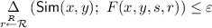
The communication complexity of the $\mathsf {CDS}$ protocol is $(\log {\left| \mathcal {T}_1 \right| } + \log {\left| \mathcal {T}_2 \right| })$ and its randomness complexity is $\log {\left| \mathcal {R} \right| }$. If $\delta$ and $\varepsilon$ are zeros, such a $\mathsf {CDS}$ scheme is called perfect.

By default, we let $\mathcal {X}= \mathcal {Y}= \{0,1\}^n$, $\mathcal {S}= \{0,1\}^s$, $\mathcal {R}= \{0,1\}^\rho$, $\mathcal {T}_1 = \{0,1\}^{t_1}$, and $\mathcal {T}_2 = \{0,1\}^{t_2}$ for positive integers $n, s, \rho , t_1$, and $t_2$.

Linear CDS. We say that a $\mathsf {CDS}$ scheme $(F_1, F_2)$ is linear over a finite field $\mathbb {F}$ (or simply linear) if, for any fixed input (x, y), the functions $F_1(x,s,r)$ and $F_2(y,s,r)$ are linear over $\mathbb {F}$ in the secret s and in the randomness r, where the secret, randomness, and messages are all taken to be vectors over $\mathbb {F}$, i.e., $\mathcal {R}=\mathbb {F}^\rho$, $\mathcal {S}=\mathbb {F}^s$, $\mathcal {T}_1=\mathbb {F}^{t_1}$ and $\mathcal {T}_2=\mathbb {F}^{t_2}$. (By default, we think of $\mathbb {F}$ as the binary field, though our results hold over general fields.) Such a linear CDS can be canonically represented by a sequence of matrices $(M_x)_{x\in \mathcal {X}}$ and $(M_y)_{y\in \mathcal {Y}}$ where $M_x\in \mathbb {F}^{t_1 \times (1+\rho )}$ and $M_y\in \mathbb {F}^{t_2 \times (1+\rho )}$ and $F_1(x,s,r)= M_x \cdot \begin{pmatrix}s \\ \varvec{r}\end{pmatrix}$ and $F_2(x,s,r)= M_y \cdot \begin{pmatrix}s \\ \varvec{r}\end{pmatrix}$. It is not hard to show that any linear CDS with non-trivial privacy and correctness errors (smaller than 1) is actually perfect. Moreover, the linearity of the senders also implies that the decoding function is linear in the messages (cf. [17]).⁶

Definition 2

We denote by $\mathsf {CDS} (f)$ the least communication complexity of a $\mathsf {CDS}$ protocol for f with $\frac{1}{10}$-correctness and $\frac{1}{10}$-privacy. $\mathsf {linCDS} (f)$ is defined analogously for linear $\mathsf {CDS}$ protocols.

3.2 Private Simultaneous Message Protocols

We will also need the following model of information-theoretic non-interactive secure computation that was introduced by [15], and was later named as Private Simultaneous Message (PSM) protocols by [23].

Definition 3

( $\mathsf {PSM}$ ). Let $f: \mathcal {X}\times \mathcal {Y}\rightarrow \mathcal {Z}$ be a function. We say that a pair of deterministic encoding algorithms $F_1: \mathcal {X}\times \mathcal {R}\rightarrow \mathcal {T}_1$ and $F_2: \mathcal {Y}\times \mathcal {R}\rightarrow \mathcal {T}_2$ are $\mathsf {PSM}$ for f if the function $F(x,y,r)=(F_1(x,r),F_2(y,r))$ that corresponds to the joint computation of $F_1$ and $F_2$ on a common r, satisfies the following properties:

• 1. ($\delta$-Correctness) There exists a deterministic algorithm $\mathsf {Dec}$, called decoder, such that for every input (x, y) we have that:

  $$\begin{aligned} \Pr _{r \mathop {\leftarrow }\limits ^{R}\mathcal {R}}\left[ \mathsf {Dec}(F(x,y,r)) \ne f(x,y)\right] \le \delta . \end{aligned}$$

• 2. ($\varepsilon$-Privacy) There exists a randomized algorithm (simulator) $\mathsf {Sim}$ such that for any input (x, y) it holds that:

  

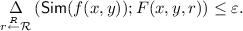
The communication complexity of the $\mathsf {PSM}$ protocol is defined as the total encoding length $(\log {\left| \mathcal {T}_1 \right| } + \log {\left| \mathcal {T}_2 \right| })$, and the randomness complexity of the protocol is defined as the length $\log {\left| \mathcal {R} \right| }$ of the common randomness. If $\delta$ and $\varepsilon$ are zeros, such a $\mathsf {PSM}$ scheme is called perfect. The scheme is balanced [6] if the simulator maps the uniform distribution over $\mathcal {Z}$ to the uniform distribution over $\mathcal {T}=\mathcal {T}_1\times \mathcal {T}_2$ and the decoder maps the uniform distribution over $\mathcal {T}$ to the uniform distribution over $\mathcal {Z}$.

3.3 Randomized Encoding and CDS Encoding

When talking about $\mathsf {PSM}$ protocols, we will use F(x, y, r) as abbreviation for $(F_1(x,r),F_2(y,r))$, and analogously for $\mathsf {CDS}$. When we do not need to explicitly argue about the common randomness, we will suppress it as an argument to F – that is, we will use F(x, y) to denote the random variable produced by F(x, y, r) for uniformly random r. Moreover, observe that the correctness and privacy conditions of both PSM and CDS are phrased as properties of the joint mapping F. One can therefore consider a non-decomposable CDS/PSM F which respects privacy and correctness, but (possibly) fails to decompose into an x-part and a y-part (i.e., some of its outputs depend both on x and y). In this case, we can ignore the partition of the input into x, y and parse them as a single argument $w=(x,y)$. Following [6, 24] we refer to this generalization of PSM as randomized encoding of f, and to the generalized version of CDS as a CDS-encoding of f. The notion of perfect and balanced PSM and perfect and linear CDS carry naturally to this setting as well. These non-decomposable variants can be trivially realized (for PSM set $F(x,y)=f(x,y)$ and for CDS take $F(x,y,s)=f(x,y)\wedge s$). Nevertheless, they offer a useful abstraction. In particular, we will use these non-decomposable notions as a useful stepping stone towards obtaining a decomposable realization.

4 Closure Properties

In this section, we establish several closure properties of CDS. We begin with closure under complement for linear CDS, then, extend the result to general CDS, and finally, prove that general and linear CDS are closed under $\mathbf {NC}^1$ circuits (or equivalently under Boolean formulas).

4.1 Reversing Linear $\mathsf {CDS}$

We begin by proving Theorem 1 (restated here for the convenience of the reader).

Theorem 7

(Linear CDS is closed under complement). Let f be a function that has a linear $\mathsf {CDS}$ scheme F with randomness complexity of $\rho$ field elements and communication complexity of t field elements. Then, the complement function $\overline{f}\equiv 1-f$ has a linear $\mathsf {CDS}$ scheme with randomness complexity of $(t+\rho +1)$ field elements and communication complexity of $2(\rho +1)$ field elements.

Proof

Let $F_1,F_2$ be a linear $\mathsf {CDS}$ scheme for f with randomness complexity $\rho$ and total communication complexity $t=t_1+t_2$, where $t_1$ is the output length of $F_1$ and $t_2$ is the output length of $t_2$. Due to linearity, we can assume that $F_1(x,s,\varvec{c})$ and $F_2(y,s,\varvec{c})$ are computed by applying matrices $M_x$ and $M_y$ to the vector $\begin{pmatrix}s \\ \varvec{c}\end{pmatrix}$, respectively. We parse $M_x = (\varvec{v}_x | T_x)$ and $M_y = (\varvec{v}_y | T_y)$, i.e., $\varvec{v}_x$ (resp., $\varvec{v}_y$) denotes the first column of $M_x$ (resp., $M_y$), and $T_x$ (resp., $T_y$) denotes the remaining columns. In the following we fix x, y to be some inputs and let $\varvec{v}= \begin{pmatrix}\varvec{v}_x \\ \varvec{v}_y\end{pmatrix}$, $T = \begin{pmatrix}T_x \\ T_y\end{pmatrix}$, $M = (\varvec{v}| T)$.

One can observe that due to the linearity of $\mathsf {CDS}$, it holds that $f(x,y)=0$ if and only if $\varvec{v}\in \mathsf {colspan} (T)$. Indeed, the joint distribution of the messages, $M \begin{pmatrix}s \\ \varvec{c}\end{pmatrix}$, is uniform over the subspace $\mathcal {U}_s=\mathsf {colspan} (T)+s\varvec{v}$. If $\varvec{v}\in \mathsf {colspan} (T)$ the subspace $\mathcal {U}_s$ collapses to $\mathsf {colspan} (T)$ regardless of the value of s (and so we get perfect privacy), whereas for $\varvec{v}\notin \mathsf {colspan} (T)$, different secrets $s\ne s'$ induce disjoint subspaces $\mathcal {U}_s$ and $\mathcal {U}_{s'}$, and so the secret can be perfectly recovered.

Based on this observation, one can construct a non-decomposable $\mathsf {CDS}$ for $\overline{f}$ (in which Alice and Bob are viewed as a single party) as follows. Compute a random mask $\varvec{\alpha }^T \varvec{v}$ (where $\varvec{\alpha }$ is a random vector), and output the masked secret bit $d = s + \varvec{\alpha }^T \varvec{v}$ together with the row vector $\varvec{\gamma }= \varvec{\alpha }^T T$. The decoding procedure starts by finding a vector $\varvec{z}$ such that $\varvec{v}= T \varvec{z}$ (such a vector always exists since $\varvec{v}\in \mathsf {colspan} (T)$ if $f(x,y)=0$), and then outputs $d - \varvec{\gamma }\varvec{z}= s + \varvec{\alpha }^T \varvec{v}- (\varvec{\alpha }^T T) \varvec{z}= s$. Of course, the resulting scheme is not decomposable, however, we can fix this problem by letting Alice and Bob compute a PSM of it. We proceed with a formal description.

We construct $\mathsf {CDS}$ scheme $G=(G_1,G_2)$ for $\overline{f}$ as follows: Alice and Bob get shared randomness $q=(u,\varvec{w},\varvec{\alpha }_1,\varvec{\alpha }_2)$, where $u \in \mathbb {F}$, $\varvec{w}\in \mathbb {F}^{\rho }$, and $\varvec{\alpha }_1 \in \mathbb {F}^{t_1}, \varvec{\alpha }_2 \in \mathbb {F}^{t_2}$. Then they compute

$$\begin{aligned} G_1(x,s,q) = (\varvec{\alpha }_1^T T_x + \varvec{w}^T, \varvec{\alpha }_1^T \cdot \varvec{v}_x + u + s) \end{aligned}$$

and

$$\begin{aligned} G_2(y,s,q)= (\varvec{\alpha }_2^T T_y-\varvec{w}^T, \varvec{\alpha }_2^T \cdot \varvec{v}_y - u). \end{aligned}$$

The decoder on input $(\varvec{m}_1,b_1)$ from Alice and $(\varvec{m}_2,b_2)$ from Bob does the following: it finds a vector $\varvec{z}$ such that $\varvec{v}= T \varvec{z}$ and outputs $b_1 + b_2 - (\varvec{m}_1 + \varvec{m}_2) \cdot \varvec{z}$.

We now prove that the pair $(G_1,G_2)$ is a $\mathsf {CDS}$ for $\overline{f}$ starting with correctness. Fix an input (x, y) for which $f(x,y)=0$. Recall that in this case $\varvec{v}\in \mathsf {colspan} (T)$, and so the decoder can find $\varvec{z}$ as required. It is not hard to verify that in this case the decoding formula recovers the secret. Indeed, letting $\varvec{\alpha }= \begin{pmatrix}\varvec{\alpha }_1 \\ \varvec{\alpha }_2\end{pmatrix}$, we have

$$\begin{aligned} b_1 + b_2 - (\varvec{m}_1 + \varvec{m}_2) \cdot \varvec{z}= s + \varvec{\alpha }^T \cdot \varvec{v}- (\varvec{\alpha }^T \cdot T) \cdot \varvec{z}= s + \varvec{\alpha }^T \cdot \varvec{v}- \varvec{\alpha }^T \cdot \varvec{v}= s. \end{aligned}$$

We now turn to proving the perfect privacy of the protocol. Consider any (x, y) such that $f(x,y) = 1$ and let $M=(\varvec{v}| T)$ be the joint linear mapping. To prove privacy, it suffices to show that, for random $\varvec{\alpha }\mathop {\leftarrow }\limits ^{R}\mathbb {F}^{t}$, the first entry of the vector $\varvec{\alpha }^T M$ is uniform conditioned on the other entries of the vector. To see this, first observe that $\varvec{\alpha }^T M$ is distributed uniformly subject to the linear constraints $\varvec{\alpha }^T M \cdot \varvec{r}=\mathbf {0}$ induced by all vectors $\varvec{r}$ in the Kernel of M. Therefore, $\varvec{\alpha }^T \varvec{v}$ is uniform conditioned on $\varvec{\alpha }^T T$ if and only if all $\varvec{r}$’s in the Kernel of M have 0 as their first entry. Indeed, if this is not the case, then $\varvec{v}\in \mathsf {colspan} (T)$, and so (x, y) cannot be 1-input of f.

Finally, observe that the protocol consumes $(t+\rho +1)$ field elements for the joint randomness, and communicates a total number of $2\rho +2$ field elements.    $\square$

4.2 Reversing General $\mathsf {CDS}$

We continue by proving Theorem 2 (restated below).

Theorem 8

(CDS is closed under complement). Suppose that f has a $\mathsf {CDS}$ with randomness complexity of $\rho$ and communication complexity of t and privacy/correctness errors of $2^{-k}$. Then $\overline{f}\equiv 1-f$ has a $\mathsf {CDS}$ scheme with similar privacy/correctness errors and randomness/communication complexity of $O(k^3\rho ^2t+k^3\rho ^3)$.

We begin with the following reversing transformation of Sahai and Vadhan [34, Corollary 4.18].

Construction 9

(Statistical Distance Reversal). Let $D^0,D^1:Q\rightarrow L$ be a pair of functions where $Q=\{0,1\}^\rho$ and $L=\{0,1\}^{t}$. For a parameter k, let $m=k^3 \rho ^2$, and let $\mathcal {H}=\left\{ h:\{0,1\}^m \times Q^m \times L^m \rightarrow S\right\}$ be a family of 2-universal hash functions where $S=\{0,1\}^{(\rho +1)m-2(m/k)-k}$. The functions $C^0$ and $C^1$ take an input $({\varvec{b}},{\varvec{r}},{\varvec{b}}',{\varvec{r}}',h, u) \in \bigl (\{0,1\}^m \times Q^m\bigr )^2 \times \mathcal {H}\times U$, and output the tuple

$$\begin{aligned} (D^{{\varvec{b}}}({\varvec{r}}), {\varvec{b}}, h,z) \end{aligned}$$

where $D^{{\varvec{b}}}({\varvec{r}})=:(D^{b_1}(r_1),\ldots ,D^{b_{m}}(r_m)),$ and

$$z = {\left\{ \begin{array}{ll} h({\varvec{b}},{\varvec{r}}, D^{{\varvec{b}}'}({\varvec{r}}')) &{} \quad for\ C^0\\ u &{} \quad for\ C^1 \end{array}\right. }.$$

In the following, we denote by $D^0$ (resp., $D^1,C^0,C^1$) the probability distributions induced by applying the function $D^0$ (resp., $D^1, C^0$, $C^1$) to a uniformly chosen input.

Fact 10

(Corollary 4.18 in [34]). In the set-up of Construction 9, the following holds for every parameter k.

• 1. If then .

• 2. If , then .

Fact 10 allows to transform a CDS $F(x,y,s,r)=(F_1(x,s;r),F_2(y,s;r))$ for the function f, into a CDS encoding C for $\overline{f}$. For inputs x, y and secret s, the CDS encoding C samples a message from the distribution $C_{xy}^s$ obtained by applying Construction 9 to the distributions $D^0_{xy}=F(x,y,0,r)$ and $D^1_{xy}=F(x,y,1,r)$.

Unfortunately, the resulting CDS encoding is not decomposable since the hash function is applied jointly to the x-th and y-th components of the distributions $D_{xy}^0$ and $D_{xy}^1$. We fix the problem by using a PSM of h. Let us begin with the following more general observation that shows that h can be safely replaced with its randomized encoding.

Lemma 1

Under the set-up of Construction 9, for every $h\in \mathcal {H}$ let $\hat{h}$ be a perfect balanced randomized encoding of h with randomness space V and output space $\hat{S}$. The function $E^0$ (resp., $E^1$) is defined similarly to $C^0$ (resp., $C^1$) except that the input is $({\varvec{b}},{\varvec{r}},{\varvec{b}}',{\varvec{r}}',h, v, \hat{s}) \in \bigl (\{0,1\}^m \times Q^m\bigr )^2 \times \mathcal {H}\times V \times \hat{S}$ and the output is identical except for the z-part which is replaced by

$$\hat{z}= {\left\{ \begin{array}{ll} \hat{h}({\varvec{b}},{\varvec{r}}, D^{{\varvec{b}}'}({\varvec{r}}');v) &{} \quad for \, E^0\\ \hat{s} &{} \quad for \, E^1 \end{array}\right. }.$$

Then, the conclusion of Fact 10 holds for $E^0$ and $E^1$ as well. Namely, for every parameter k,

• 1. if then ;

• 2. if , then .

Proof

Fix $D^0$ and $D^1$. We prove that and conclude the lemma from Fact 10. Indeed, consider the randomized mapping T which maps a tuple (a, b, h, z) to $(a,b,h,\mathsf {Sim}(z))$ where $\mathsf {Sim}$ is the simulator of the encoding $\hat{h}$. Then, by the perfect privacy and the balanced property, T takes $C^0$ to $E^0$ and $C^1$ to $E^1$. Since statistical distance can only decrease when the same probabilistic process is applied to two random variables, it follows that $\varDelta (C^0,C^1)\le \varDelta (T(C^0),T(C^1))=\varDelta (E^0,E^1)$. For the other direction, consider the mapping $T'$ which maps a tuple $(a,b,h,\hat{z})$ to $(a,b,h,\mathsf {Dec}(\hat{z}))$ where $\mathsf {Dec}$ is the decoder of the encoding. Then, by the perfect correctness and by the balanced property, T takes $E^0$ to $C^0$ and $E^1$ to $C^1$. It follows that $\varDelta (E^0,E^1)\le \varDelta (T'(E^0),T'(E^1))=\varDelta (C^0,C^1)$, and the lemma follows.    $\square$

We can now prove Theorem 8.

Proof

(Proof of Theorem 8 ). Let $F=(F_1,F_2)$ be a CDS for the function f with randomness complexity $\rho$, communication t and privacy/correctness error of $2^{-k}$. For inputs x, y and secret $\sigma$, the CDS for $\overline{f}$ will be based on the functions $E^{\sigma }$ defined in Lemma 1 where $D^0(r)=F(x,y,0;r)$ and $D^1(r)=F(x,y,1;r)$. In particular, we will instantiate Lemma 1 as follows.

Let

$$\begin{aligned} \alpha =({\varvec{b}},{\varvec{r}},D_{xy}^{{\varvec{b}}}({\varvec{r}})), \quad \text {where}\, D_{xy}^{{\varvec{b}}}({\varvec{r}}):=(F(x,y,b_1;r_1),\ldots ,F(x,y,b_m;r_m)) \end{aligned}$$

be the input to the hash function h. Let $n_0=m(1+\rho +t)$ denote the length of $\alpha$. Observe that each bit of $\alpha$ depends either on x or on y but not in both (since F is a CDS). Let $A\subset [n_0]$ denote the set of entries which depend on x and let $B=[n_0]\setminus A$ be its complement. Let $n_1=(\rho +1)m-2m/k-k$ denote the output length of the hash function family $\mathcal {H}$. We implement $\mathcal {H}=\left\{ h\right\}$ by using Toeplitz matrices. That is, each function is defined by a binary Toeplitz matrix $M\in \mathbb {F}_2^{n_1\times n_0}$ (in which each descending diagonal from left to right is constant) and a vector $w\in \mathbb {F}_2^{n_1}$, and $h(\alpha )=M\alpha +w$. Let us further view the hash function $h(\alpha )$ as a two-argument function $h(\alpha _A,\alpha _B)$ and let

$$\begin{aligned} \hat{h}(\alpha _A,\alpha _B;v)=(M_A\alpha _A+w+v,M_B\alpha _B-v), \end{aligned}$$

where $v\in \mathbb {F}_2^{n_1}$ and $M_A$ (resp. $M_B$) is the restriction of M to the columns in A (resp., columns in B). It is not hard to verify that $\hat{h}$ is a perfect balanced PSM for h. (Indeed decoding is performed by adding Alice’s output to Bob’s output, and simulation is done by splitting an output $\beta$ of h into two random shares $c_1,c_2\in \mathbb {F}_2^{n_1}$ which satisfy $c_1+c_2=\beta$.)

Consider the randomized mapping $E_{xy}^{\sigma }$ obtained from Lemma 1 instantiated with $D^s(r)=D^s_{xy}(r)=F(x,y,s;r)$ and the above choices of $\hat{h}$. We claim that $E_{xy}^{\sigma }$ is a CDS for $\overline{f}$ with privacy and correctness error of $2^{-k}$. To see this first observe that, by construction, the output of $E_{xy}^{\sigma }$ can be decomposed into an x-component $E_1(x,\sigma )$ and a y-component $E_2(y,\sigma )$. (All the randomness that is used as part of the input to E is consumed as part of the joint randomness of the CDS.)

To prove privacy, fix some 0-input (x, y) of $\overline{f}$ and note that $f(x,y)=1$ and therefore, by the correctness of the CDS F, it holds that . We conclude, by Lemma 1, that and privacy holds. For correctness, fix some 1-input (x, y) of $\overline{f}$ and note that $f(x,y)=0$ and therefore, by the privacy of the CDS F, it holds that . We conclude, by Lemma 1, that and so correctness holds (by using the optimal distinguisher as a decoder). Finally, since the description length of h is $n_0+2n_1$ the randomness complexity of $\hat{h}$ is $n_1$ and the communication complexity of $\hat{h}$ is $2n_1$, the overall communication and randomness complexity of the resulting CDS is $O(k^3\rho ^2t+k^3\rho ^3)$.    $\square$

4.3 Closure Under Formulas

Closure under formulas can be easily deduced from Theorems 7 and 8.

Theorem 11

Let g be a Boolean function over m binary inputs that can be computed by a $\sigma$-size formula. Let $f_1,\ldots ,f_m$ be m boolean functions over $\mathcal {X}\times \mathcal {Y}$ each having a $\mathsf {CDS}$ with t communication and randomness complexity, and $2^{-k}$ privacy and correctness errors. Then, the function $h: \mathcal {X}\times \mathcal {Y}\rightarrow \left\{ 0,1\right\}$ defined by $g(f_1(x,y),\ldots ,f_m(x,y))$ has a $\mathsf {CDS}$ scheme with $O(\sigma k^3t^3)$ randomness and communication complexity, and $\sigma 2^{-k}$ privacy and correctness errors. Moreover, in the case of linear CDS, the communication and randomness complexity are only $O(\sigma t)$ and the resulting CDS is also linear.

Proof

Without loss of generality, assume that the formula g is composed of AND and OR gates and all the negations are at the bottom (this can be achieved by applying De Morgan’s laws) and are not counted towards the formula size. We prove the theorem with an upper-bound of $\sigma \cdot C k^3t^3$ where C is the constant hidden in the big-O notation in Theorem 8 (the upper-bound on the communication/randomness complexity of the complement of a CDS).

The proof is by induction on $\sigma$. For $\sigma =1$, the formula g is either $f_i(x,y)$ or $\overline{f}_i(x,y)$ for some $i\in [m]$, in which case the claim follows either from our assumption on the CDS for $f_i$ or from Theorem 8. To prove the induction step, consider a $\sigma$-size formula $g(f_1,\ldots ,f_m)$ of the form $g_1(f_1,\ldots ,f_m) \diamond g_2(f_1,\ldots ,f_m)$ where $\diamond$ is either AND or OR, $g_1$ and $g_2$ are formulas of size $\sigma _1$ and $\sigma _2$, respectively, and $\sigma =\sigma _1+\sigma _2+1$. For the case of an AND gate, we additively secret share the secret s into random $s_1$ and $s_2$ subject to $s_1+ s_2=s$ and use a CDS for $g_1$ with secret $s_1$ and for $g_2$ for the secret $s_2$. For the case of OR gate, use a CDS for $g_1$ with secret s and for $g_2$ for the secret s. By the induction hypothesis, the communication and randomness complexity are at most $\sigma _1\cdot C k^3t^3+\sigma _2\cdot C k^3t^3+1\le \sigma C k^3t^3$, and the privacy/correctness error grow to $\sigma _1 2^{-k}+ \sigma _2 2^{-k}\le \sigma 2^{-k}$, as required.

The extension to the linear case follows by plugging the upper-bound from Theorem 7 to the basis of the induction, and by noting that the construction preserves linearity.    $\square$

5 Amplifying Correctness and Privacy of $\mathsf {CDS}$

In this section we show how to simultaneously reduce the correctness and privacy error of a $\mathsf {CDS}$ scheme F. Moreover, the transformation has only minor cost when applied to long secrets.

Theorem 12

Let $f:X\times Y \rightarrow \{0,1\}$ be a predicate and let F be a $\mathsf {CDS}$ for f which supports 1-bit secrets with correctness error $\delta _0=0.1$ and privacy error $\varepsilon _0=0.1$. Then, for every integer k there exists a $\mathsf {CDS}$ G for f with k-bit secrets, privacy and correctness errors of $2^{-\varOmega (k)}$. The communication (resp., randomness) of G larger than those of F by a multiplicative factor of O(k).

Proof

Let $\varepsilon$ be some constant larger than $\varepsilon _0$. Let $\mathsf {E}$ be a randomized mapping that takes k-bit message s and O(k)-bit random string into an encoding c of length $m=\varTheta (k)$ with the following properties:

• 1. If one flips every bit of $\mathsf {E}(s)$ independently at random with probability $\delta _0$ then s can be recovered with probability $1-\exp (-\varOmega (k))$.

• 2. For any pair of secrets s and $s'$ and any set $T\subset [m]$ of size at most $\varepsilon m$, the T-restricted encoding of s is distributed identically to the T-restricted encoding of $s'$, i.e., $(\mathsf {E}(s)_{i})_{i\in T}\equiv (\mathsf {E}(s')_{i})_{i\in T}$.

That is, $\mathsf {E}$ can be viewed as a ramp secret-sharing scheme with 1-bit shares which supports robust reconstruction.⁷ Such a scheme can be based on any linear error-correcting code with good dual distance [13]. In particular, by using a random linear code, we can support $\varepsilon _0=\delta _0=0.1$ or any other constants which satisfy the inequality $1-H_2(\delta _0)>H_2(\varepsilon _0)$.

Given the CDS $F=(F_1,F_2)$ we construct a new CDS $G=(G_1,G_2)$ as follows. Alice and Bob jointly map the secret $s\in \{0,1\}^k$ to $c=\mathsf {E}(s;r_0)$ (using joint randomness $r_0$). Then, for every $i\in [m]$, Alice outputs $F_1(x,c_i;r_i)$ and Bob outputs $F_2(y,c_i;r_i)$, where $r_1,\ldots ,r_m$ are given as part of the shared randomness.

Let us analyze the correctness of the protocol. Fix some x, y for which $f(x,y)=1$. Consider the decoder which given $(v_1,\ldots ,v_m)$ and x, y applies the original decoder of F to each coordinate separately (with the same x, y), and passes the result $\hat{c}\in \{0,1\}^{m}$ to the decoding procedure of $\mathsf {E}$, promised by Property (1) above. By the correctness of F, each bit $\hat{c}_i$ equals to $c_i$ with probability of at least $1-\delta _0$. Therefore, the decoder of $\mathsf {E}$ recovers c with all but $1-\exp (-\varOmega (k))$ probability.

Consider the simulator which simply applies G to the secret $s'=0^k$. Fix x and y and a secret s. To upper-bound the statistical distance between $G(x,y,s')$ and G(x, y, s), we need the following standard “coupling fact” (cf. [30, Lemma 5] for a similar statement).

Fact 13

Any pair of distributions, $(D_0,D_1)$ whose statistical distance is $\varepsilon$ can be coupled into a joint distribution $(E_0,E_1,b)$ with the following properties:

• 1. The marginal distribution of $E_0$ (resp., $E_1$) is identical to $D_0$ (resp., $D_1$).

• 2. b is an indicator random variable which takes the value 1 with probability $\varepsilon$.

• 3. Conditioned on $b=0$, the outcome of $E_0$ equals to the outcome of $E_1$.

Define the distributions $D_0:=F(x,y,0)$ and $D_1:=F(x,y,1)$, and let $(E_0,E_1,b)$ be the coupled version of $D_0,D_1$ derived from Fact 13. Let $c=\mathsf {E}(s)$ and $c'=\mathsf {E}(s')$. Then,

$$\begin{aligned} G(x,y,s)=(E^1_{c_1}, \ldots , E^m_{c_m}), \end{aligned}$$

and

$$\begin{aligned} G(x,y,s')=(E^1_{c'_1}, \ldots , E^m_{c'_m}), \end{aligned}$$

where for each $i\in [m]$ the tuple $(E^i_0,E^i_1,b^i)$ is sampled jointly and independently from all other tuples. Let $T=\left\{ i\in [m]: b_i\ne 0\right\}$. Then, it holds that

$$\begin{aligned} \varDelta (G(x,y,s); G(x,y,s'))&\le \varDelta ((T,(E^i_{c_i})_{i\in T}) ; (T,(E^i_{c'_i})_{i\in T}))\\&\le \Pr [|T|> \varepsilon m] \le \exp (-\varOmega (k)), \end{aligned}$$

where the first inequality follows from Fact 13, the second inequality follows from the second property of $\mathsf {E}$ and the last inequality follows from a Chernoff bound (recalling that $\varepsilon -\varepsilon '>0$ is a constant and $m=\varTheta (k)$). The theorem follows.    $\square$

Remark 1

(Optimization). The polarization lemma of Sahai and Vadhan [34] provides an amplification procedure which works for a wider range of parameters. Specifically, their transformation can be applied as long as the initial correctness and privacy errors satisfy the relation $\delta _0^2>\varepsilon _0$. (Some evidence suggest that this condition is, in fact, necessary for any amplification procedure [22].) Unfortunately, the communication overhead in their reduction is polynomially larger than ours and does not amortize over long secrets. It is not hard to combine the two approaches and get the best of both worlds. In particular, given a CDS with constant correctness and privacy errors which satisfy $\delta _0^2>\varepsilon _0$, use the polarization lemma with constant security parameter $k_0$ to reduce the errors below the threshold needed for Theorem 12, and then use the theorem to efficiently reduce the errors below $2^{-k}$. The resulting transformation has the same asymptotic tradeoff between communication, error, and secret length, and can be used for a wider range of parameters. (This, in particular, yields the statement of Theorem 3 in the introduction in which $\delta _0$ and $\varepsilon _0$ are taken to be 1/3.)

Remark 2

(Preserving efficiency). Theorem 12 preserves efficiency (of the CDS senders and decoder) as long as the encoding $\mathsf {E}$, and its decoding algorithm are efficient. This can be guaranteed by replacing the random linear codes (for which decoding is not know to be efficient) with an Algebraic Geometric Codes (as suggested in [13]; see also Claim 4.1 in [25] and [12, 16]). This modification requires to start with smaller (yet constant) error probabilities $\delta _0,\varepsilon _0$. As in Remark 1, this limitation can be easily waived. First use the inefficient transformation (based on random binary codes) with constant amplification $k_0=O(1)$ to reduce the privacy/correctness error below the required threshold, and then use the efficient amplification procedure (based on Algebraic Geometric Codes).

6 Amortizing the Communication for Long Secrets

In this section we show that, for sufficiently long secrets, the amortized communication cost of CDS for n-bit predicates is O(n) bits per each bit of the secret. As explained in the introduction, in order to prove this result we first amortize CDS over many different predicates (applied to the same input (x, y)). We refer to this version of CDS as batch-CDS, formally defined below.

Definition 4

(batch- $\mathsf {CDS}$ ). Let $\mathcal {F}=(f_1,\ldots ,f_m)$ be an m-tuple of predicates over the domain $\mathcal {X}\times \mathcal {Y}$. Let $F_1 : \mathcal {X}\times \mathcal {S}^m \times \mathcal {R}\rightarrow \mathcal {T}_1$ and $F_2 : \mathcal {Y}\times \mathcal {S}^m \times \mathcal {R}\rightarrow \mathcal {T}_2$ be deterministic encoding algorithms, where $\mathcal {S}$ is the secret domain (by default $\{0,1\}$). Then, the pair $(F_1,F_2)$ is a batch-$\mathsf {CDS}$ scheme for $\mathcal {F}$ if the function $F(x,y,s,r)=(F_1(x,s,r),F_2(y,s,r))$, that corresponds to the joint computation of $F_1$ and $F_2$ on a common s and r, satisfies the following properties:

• 1. (Perfect correctness)⁸ There exists a deterministic algorithm $\mathsf {Dec}$, called a decoder, such that for every $i\in [m]$, every 1-input (x, y) of $f_i$ and every vector of secrets $s \in \mathcal {S}^m$, we have that:

  $$\begin{aligned} \Pr _{r \mathop {\leftarrow }\limits ^{R}\mathcal {R}}[\mathsf {Dec}(i,x,y,F(x,y,s,r)) = s_i] =1. \end{aligned}$$

• 2. (Perfect privacy) There exists a simulator $\mathsf {Sim}$ such that for every input (x, y) and every vector of secrets $s \in \mathcal {S}^m$, the following distributions are identical

  $$\begin{aligned} \mathsf {Sim}(x,y,\hat{s}) \qquad \text {and} \qquad F(x,y,s,r), \end{aligned}$$

  where $r\mathop {\leftarrow }\limits ^{R}\mathcal {R}$ and $\hat{s}$ is an m-long vector whose i-th component equals to $s_i$ if $f_i(x,y)=1$, and $\bot$ otherwise.

The communication complexity of the $\mathsf {CDS}$ protocol is $(\log {\left| \mathcal {T}_1 \right| } + \log {\left| \mathcal {T}_2 \right| })$.

In the following, we let $\mathcal {F}_n$ denote the $2^{2^{2n}}$-tuple which contains all predicates $f:\{0,1\}^n\times \{0,1\}^n\rightarrow \{0,1\}$ defined over pairs of n-bit inputs (sorted according to some arbitrary order).

Lemma 2

$\mathcal {F}_n$-batch CDS can be implemented with communication complexity of $3|\mathcal {F}_n|$. Moreover the protocol is linear.

Proof

The proof is by induction on n. For $n=1$, it is not hard to verify that any predicate $f:\{0,1\}\times \{0,1\}\rightarrow \{0,1\}$ admits a CDS with a total communication complexity of at most 2 bits. Indeed, there are 16 such predicates, out of which, six are trivial in the sense that the value of f depends only in the inputs of one of the parties (and so they admit a CDS with 1 bit of communication), and the other ten predicates correspond, up to local renaming of the inputs, to AND, OR, and XOR, which admit simple linear 2-bit CDS as follows. For AND, Alice and Bob send $s\cdot x + r$ and $r\cdot y$; for OR, they send $x \cdot s$ and $y\cdot s$; and, for XOR, they send $s+x\cdot r_1+(1-x)r_2$ and $y\cdot r_2+(1-y)r_1$ (where r and $(r_1,r_2)$ are shared random bits and addition/multiplication are over the binary field). It follows, that $\mathcal {F}_1$-batch CDS can be implemented with total communication of at most $2|\mathcal {F}_1|$. (In fact, this bound can be improved by exploiting the batch mode.)

Before proving the induction step. Let us make few observations. For $(\alpha ,\beta )\in \{0,1\}^2$, consider the mapping $\phi _{\alpha ,\beta }:\mathcal {F}_{n+1}\rightarrow \mathcal {F}_n$ which maps a function $f\in \mathcal {F}_{n+1}$ to the function $g\in \mathcal {F}_n$ obtained by restricting f to $x_{n+1}=\alpha$ and $y_{n+1}=\beta$. The mapping $\phi _{\alpha ,\beta }$ is onto, and is D-to-1 where $D=|\mathcal {F}_{n+1}|/|\mathcal {F}_n|$. We can therefore define a mapping $T_{\alpha ,\beta }(f)$ which maps $f\in \mathcal {F}_{n+1}$ to $(g,i)\in \mathcal {F}_{n}\times [D]$ such that f is the i-th preimage of g under $\phi _{\alpha ,\beta }$ with respect to some fixed order on $\mathcal {F}_{n+1}$. By construction, for every fixed $(\alpha ,\beta )$, the mapping $T_{\alpha ,\beta }$ is one-to-one.

We can now prove the induction step; That is, we construct $\mathcal {F}_{n+1}$-batch CDS based on D copies of $\mathcal {F}_{n}$-batch CDS. Given input $x\in \{0,1\}^{n+1}$ for Alice, $y\in \{0,1\}^{n+1}$ for Bob, and joint secrets $(s_f)_{f\in \mathcal {F}_{n+1}}$, the parties proceed as follows.

• 1. Alice and Bob use D copies of $\mathcal {F}_{n}$-batch CDS with inputs $x'=(x_1,\ldots ,x_n)$ and $y'=(y_1,\ldots ,y_n)$. In the i-th copy, for every predicate $g\in \mathcal {F}_n$, a random secret $r_{g,i}\in \{0,1\}$ is being used. (The $r_{g,i}$’s are taken from the joint randomness of Alice and Bob.)

• 2. For every $f\in \mathcal {F}_{n+1}$ and $(\alpha ,\beta )\in \{0,1\}^2$, Alice and Bob release the value $\sigma _{f,\alpha ,\beta }=s_f+ r_{g,i}$ where $(g,i)=T_{\alpha ,\beta }(f)$ iff the last bits of their inputs, $x_{n+1}$ and $y_{n+1}$, are equal to $\alpha$ and $\beta$, respectively. This step is implemented as follows. For each f, Alice sends a pair of bits

  $$\begin{aligned} c_{f,0}=\sigma _{f,x_{n+1},0}+r'_{f,0}, \quad \text {and} \quad c_{f,1}=\sigma _{f,x_{n+1},1}+r'_{f,1}, \end{aligned}$$

  and Bob sends $r'_{f,y_{n+1}}$ where $r'_{f,0},r'_{f,1}$ are taken from the joint randomness.

The decoding procedure is simple. If the input $(x,y)\in \{0,1\}^{n+1}\times \{0,1\}^{n+1}$ satisfies $f\in \mathcal {F}_{n+1}$, the decoder does the following: (1) Computes $(g,i)=T_{x_{n+1},y_{n+1}}(f)$ and retrieves the value of $r_{g,i}$ which is released by the batch-CDS since $g(x',y')=f(x,y)=1$; (2) Collects the values $c_{f,x_{n+1}}$ and $r'_{f,y_{n+1}}$ sent during the second step, and recovers the value of $s_f$ by computing $c_{f,x_{n+1}}-r'_{f,y_{n+1}}-r_{g,i}$.

In addition, it is not hard to verify that perfect privacy holds. Indeed, suppose that $(x,y)\in \{0,1\}^{n+1}\times \{0,1\}^{n+1}$ does not satisfy f. Then, the only $s_f$-dependent value which is released is $s_f\oplus r_{g,i}$ where g is the restriction of f to $(x_{n+1},y_{n+1})$. However, since (x, y) fails to satisfy f, its prefix does not satisfy g and therefore $r_{g,i}$ remains hidden from the receiver. Formally, we can perfectly simulate the view of the receiver as follows. First simulate the first step using D calls to the simulator of $\mathcal {F}_{n}$-batch CDS with random secrets $r_{g,i}$. Then simulate the second step by sampling, for each f, three values $c_{f,0},c_{f,1}$ and $r'$ which are uniform if $f(x,y)=0$, and, if $f(x,y)=1$, satisfy the linear constraint $s_f=c_{f,x_{n+1}}-r'_{f,y_{n+1}}-r_{g,i}$ where $(g,i)=T_{\alpha ,\beta }(f)$.

Finally the communication complexity equals to the complexity of D copies of batch CDS for $\mathcal {F}_{n}$ (communicated in the first step) plus $3|\mathcal {F}_{n+1}|$ bits (communicated at the second step). Therefore, by the induction hypothesis, the overall communication, is $3|\mathcal {F}_{n+1}|+3Dn|\mathcal {F}_{n}|$. Recalling that $D=|\mathcal {F}_{n+1}|/|\mathcal {F}_n|$, we derive an upper-bound of $3(n+1)|\mathcal {F}_{n+1}|$, as required.    $\square$

We use Lemma 2 to amortize the complexity of CDS over long secrets.

Theorem 14

Let $f:\{0,1\}^n\times \{0,1\}^n\rightarrow \{0,1\}$ be a predicate. Then, for $m=|\mathcal {F}_{n}|/2=2^{2^{2n}}/2$, there exists a perfect linear CDS which supports m-bit secrets with total communication complexity of $12\,\mathrm{{nm}}$.

The case of longer secrets of length $m>|\mathcal {F}_n|/2$ (as in Theorem 4) can be treated by partitioning the secret to $|\mathcal {F}_{n}|/2$-size blocks and applying the CDS for each block separately. The overall communication complexity is upper-bounded by $13\,\mathrm{{nm}}$.

Proof

Given a vector S of $m=|\mathcal {F}_{n}|/2$ secrets, we duplicate each secret twice and index the secrets by predicates $p\in \mathcal {F}_n$ such that $s_p=s_{\bar{p}}$ (i.e., a predicate and its complement index the same secret). On inputs x, y, Alice and Bob make two calls to $\mathcal {F}_n$-batch CDS (with the same inputs x, y). In the first call the secret associated with a predicate $p\in \mathcal {F}_n$ is a random values $r_p$. In the second call, for every predicate $h\in \mathcal {F}_n$, we release the secret $s_p\,\oplus \,r_p$ where p is the unique predicate for which $p=f+h+1$ (where addition is over the binary field).

Correctness. Suppose that $f(x,y)=1$. Recall that each of the original secrets $S_i$ appears in two copies $(s_p,s_{\bar{p}})$ for some predicate p. Since one of these copies is satisfied by (x, y), it suffices to show that, whenever $p(x,y)=1$, the secret $s_p$ can be recovered. Indeed, for such a predicate p, the value $r_p$ is released by the first batch-CDS, and the value $s_p\,\oplus \,r_p$ is released by the second batch-CDS. The latter follows by noting that the predicate h which satisfies $p=f+h+1$ is also satisfied, since $h(x,y)=p(x,y)+f(x,y)+1=1$. It follows that $s_p$ can be recovered for every p which is satisfied by (x, y), as required.

Privacy. Suppose that $f(x,y)=0$. We show that all the “virtual secrets” $s_p$ remain perfectly hidden in this case. Indeed, for h and p which satisfy $p=f+h+1$, it holds that, whenever $f(x,y)=0$, either $h(x,y)=0$ or $p(x,y)=0$, and therefore, for any p, either $r_p$ or $s_p\,\oplus \,r_p$ are released, but never both.

Finally, using Lemma 2, the total communication complexity of the protocol is $2\cdot 3 \cdot n \cdot |\mathcal {F}_n|=12\,nm$, as claimed.    $\square$

7 A Linear Lower Bound on $\mathsf {CDS}$

Here we show that the lower bound on the communication complexity of $\mathsf {PSM}$ protocols proven in [15] can be extended to apply for $\mathsf {CDS}$ as well. We do this by showing how to use $\mathsf {CDS}$ protocols to construct $\mathsf {PSM}$ protocols that are only required to hide a certain small pre-specified set of input bits (as opposed to the whole input). We define this notion of $\mathsf {PSM}$ below.

Definition 5

(b-bit $\mathsf {PSM}$ ). Consider a function $f: (\mathcal {W}\times \mathcal {X}) \times \mathcal {Y}\rightarrow \mathcal {Z}$, with $\log {\left| \mathcal {W} \right| } \ge b$ for some $b > 0$. We say that a pair of deterministic encoding algorithms $F_1: \mathcal {W}\times \mathcal {X}\times \mathcal {R}\rightarrow \mathcal {T}_1$ and $F_2: \mathcal {Y}\times \mathcal {R}\rightarrow \mathcal {T}_2$ constitute a $b\text {-bit}\ \mathsf {PSM}$ for f if the function $F((w,x),y,r)=(F_1(w,x,r),F_2(y,r))$ satisfies the following properties:

• 1. ($\delta$-Correctness): There exists a deterministic algorithm $\mathsf {Dec}$, called the decoder, such that for every input ((w, x), y) we have that:

  $$\begin{aligned} \Pr _{r \mathop {\leftarrow }\limits ^{R}\mathcal {R}}[\mathsf {Dec}(F((w,x),y,r)) \ne f((w,x),y)] \le \delta . \end{aligned}$$

• 2. (b-bit $\varepsilon$-Privacy): There exists a randomized algorithm $\mathsf {Sim}$ such that for any input ((w, x), y) it holds that:

  

The communication complexity of the protocol is defined as the total encoding length $(\log {\left| \mathcal {T}_1 \right| }+\log {\left| \mathcal {T}_2 \right| })$, and the randomness complexity of the protocol is defined as $\log {\left| \mathcal {R} \right| }$.

By default, the above sets are to be taken to be $\mathcal {W}= \{0,1\}^b$, $\mathcal {X}= \mathcal {Y}= \{0,1\}^n$, $\mathcal {Z}= \{0,1\}$, $\mathcal {R}= \{0,1\}^\rho$, $\mathcal {T}_1 = \{0,1\}^{t_1}$, and $\mathcal {T}_2 = \{0,1\}^{t_2}$ for some positive integers $b, n, \rho , t_1$, and $t_2$.

Lemma 3

( $\mathsf {CDS}$ to 1-bit $\mathsf {PSM}$ ). If every Boolean function on $\mathcal {X}\times \mathcal {Y}$ has a $\mathsf {CDS}$ protocol with communication complexity t, then every Boolean function on $(\{0,1\}\times \mathcal {X})\times \mathcal {Y}$ has a $1\text {-bit}\ \mathsf {PSM}$ protocol with communication complexity $(t+1+\log {\left| \mathcal {X} \right| }+\log {\left| \mathcal {Y} \right| })$, with the same correctness and privacy guarantees.

Proof

Suppose we want to construct a $1\text {-bit}\ \mathsf {PSM}$ protocol for a function $f:(\{0,1\}\times \mathcal {X})\times \mathcal {Y}\rightarrow \{0,1\}$. Let $(G_1, G_2, \mathsf {Dec}_\mathsf {CDS})$ be a $\mathsf {CDS}$ protocol for the function $g(x,y) = f((0,x),y)\,\oplus \,f((1,x),y)$ with communication complexity t.

We use this to construct our $1\text {-bit}\ \mathsf {PSM}$ protocol $(F_1, F_2, \mathsf {Dec})$ for f. Let s be a bit from the common randomness. $F_1$ is now defined as $F_1((w, x), (s,r)) = (G_1(x, s, r), w\,\oplus \,s, x)$, and $F_2$ is defined as $F_2(y, (s,r)) = (G_2(y, s, r), y)$.

$\mathsf {Dec}$, on input $((g_1, w\oplus s, x), (g_2, y))$, works by first checking whether given x and y, the value of f still depends on w. If not, it simply computes f using x and y. If it does depend on w, this implies that $f((0,x),y) \ne f((1,x),y)$, and $g(x,y) = 1$, and so $\mathsf {Dec}_\mathsf {CDS} (x, y, g_1, g_2)$ outputs s, which can be used to retrieve w from $(w\,\oplus \,s)$, and now the whole input is known and f can be computed. This argues correctness, and the error here is at most that in the $\mathsf {CDS}$ protocol. The communication is also seen to be at most $(t+\log {\left| \mathcal {X} \right| }+\log {\left| \mathcal {Y} \right| }+1)$.

Let $\mathsf {Sim}_\mathsf {CDS}$ be the simulator for the $\mathsf {CDS}$ protocol for g. The simulator $\mathsf {Sim}(f((w,x),y),x,y)$ works by first checking whether $f((0,x),y) = f((1,x),y)$. If it isn’t, then the value of w is determined by x, y, and the value of f and, knowing w, $\mathsf {Sim}$ can compute $F_1$ and $F_2$ by itself, thus simulating them perfectly. If not, this implies that $g(x, y) = 0$. In this case, $\mathsf {Sim}$ first computes $(g_1^*, g_2^*) \leftarrow \mathsf {Sim}_\mathsf {CDS} (x, y)$, picks a random bit $s^*$, and outputs $((g_1^*, s^*, x), (g_2^*, y))$. The simulation error is:

Note that here $s^*$ and $(w\oplus s)$ have the same marginal distribution, which is the uniform distribution over $\{0,1\}$. Also, $\mathsf {Sim}_\mathsf {CDS} (x,y)$ is independent of $s^*$. Writing out the expansion of in terms of differences in probabilities and using Bayes’ Theorem along with the above observation gives us the following:

By the $\varepsilon$-privacy of the $\mathsf {CDS}$ scheme (since the value of g(x, y) is 0), each summand in the right-hand side above is at most $\varepsilon$. Hence the total simulation error is at most $\varepsilon$.    $\square$

In [15] it was shown that there exists a Boolean function on $\{0,1\}^n\times \{0,1\}^n$ such that any perfect $1\text {-bit}\ \mathsf {PSM}$ for it requires at least 2.99n bits of communication. Using Lemma 3 along with this lower bound, we have the following theorem.

Theorem 15

There is a Boolean function on $\{0,1\}^n\times \{0,1\}^n$ such that any perfect $\mathsf {CDS}$ protocol for it has communication complexity at least 0.99n.

We can generalise the above approach to construct $b\text {-bit}\ \mathsf {PSM}$ protocols for larger values of b as follows.

Lemma 4

( ${\mathsf {CDS}}$ to b-bit $\mathsf {PSM}$ ). If every Boolean function on $\mathcal {X}\times \mathcal {Y}$ has a $\mathsf {CDS}$ protocol with communication complexity t then, for any $b > 0$, every Boolean function on $(\{0,1\}^b\times \mathcal {X})\times \mathcal {Y}$ has a $b\text {-bit}\ \mathsf {PSM}$ protocol with communication complexity $(2^{2^b}(t+1)+\log {\left| \mathcal {X} \right| }+\log {\left| \mathcal {Y} \right| })$, with the same correctness guarantee and with privacy that is degraded by a factor of $2^{2^b}$.

Proof

(Proof sketch). The idea behind the construction is that the function $f_{x,y}(w) = f((w,x),y)$, where w is b bits long, can be one of only $2^{2^b}$ functions – call this set of functions $\mathcal {H} = \{h_i\}$. For each of these $h_i$’s, we define a function $g_i(x,y)$ that indicates whether $f_{x,y} \equiv h_i$. Note that once the $\mathsf {PSM}$ decoder knows x and y, the information that the value of f reveals to it about w is exactly $f_{x,y}(w)$, which is the same as $h_i(w)$ if $g_i(x,y) = 1$.

In our construction, first we have $F_1$ reveal x and $F_2$ reveal y. Now we wish to, for each i, reveal $h_i(w)$ if and only if $g_i(x,y) = 1$. To do this, for each i, we choose a random bit $s_i$ from the common randomness, reveal $h_i(w)\,\oplus \,s_i$, and run the $\mathsf {CDS}$ protocol for $g_i$ with $s_i$ as the secret.

The correctness is preserved because whenever the $\mathsf {CDS}$ for the “correct” value of i is correct, our protocol is correct.

The simulator, given x, y and f((w, x), y), first outputs x and y. It then finds the $i'$ such that $g_{i'}(x,y) = 1$. For every other i, it publishes a random $s_i^*$ and the output of the $\mathsf {CDS}$ simulator for the function $g_i$ with inputs x, y and secret 0. For $i'$, it publishes $(f((w,x),y)\oplus s_{i'}^*)$ for a random $s_{i'}^*$ and the messages of the $\mathsf {CDS}$ protocol for $g_{i'}$ with inputs x, y and secret $s_{i'}^*$. Privacy error goes from $\varepsilon$ to $2^{2^b}\varepsilon$ because of arguments similar to those in the proof of Lemma 3 being applied to each invocation of the $\mathsf {CDS}$ protocol, all of which are mutually independent.    $\square$

8 Separating $\mathsf {CDS}$ and Insecure Communication

Here we show an explicit function whose randomized communication complexity is much higher than its $\mathsf {CDS}$ communication complexity. For simplicity, assume that n below is a power of 2; the statements made here can be shown to be true for a general n along the same lines.

Definition 6

(Communication Complexity). Consider a function $f:\mathcal {X}\times \mathcal {Y}\rightarrow \mathcal {Z}$. A protocol between two parties (with shared randomness) who are given inputs $x\in \mathcal {X}$ and $y\in \mathcal {Y}$, respectively, is said to compute f if for every $(x,y) \in \mathcal {X}\times \mathcal {Y}$, the parties arrive at the correct value of f at the end of it with probability at least 2/3.

The communication cost of a protocol is the most number of bits exchanged by the parties over all possible inputs and all values of shared randomness. The Randomized Communication Complexity of f, denoted $\mathsf {R} (f)$, is the least communication cost of any protocol computing f.

Gay et al. [17] showed that if a function has a $\mathsf {CDS}$ protocol with communication complexity t then, roughly, $\log \mathsf {R} (f) \le 2t$. Moreover, this upper-bound can be achieved by a one-way communication protocol (in which only one party sends a message). We show that this bound is optimal (up to constant factors) by exhibiting a function that has a $\mathsf {CDS}$ protocol with low communication, but has high randomized communication complexity (even for fully interactive protocols).⁹ Towards this, we first introduce the following problem.

Definition 7

(The Collision Problem). The Collision Problem $(\mathsf {Col} _n)$ is a promise problem defined over a subset of $\{0,1\}^{n\log n}$ as follows. For an input $x \in \{0,1\}^{n\log n}$, divide x into n blocks of $\log n$ bits each. Each such x can now be used to define a function $f_x:\{0,1\}^{\log n}\rightarrow \{0,1\}^{\log n}$, where $f_x(i)$ is the $i^{\text {th}}$ block of x (when i is interpreted as an integer in [n]). $\mathsf {Col} _n(x)$ is defined to be 1 if $f_x$ is a permutation, 0 if $f_x$ is 2-to-1, and is undefined otherwise.

We use the above problem in conjunction with Sherstov’s Pattern Matrix method [36] for proving communication complexity lower bounds. We define the following function that corresponds to what would be called a “pattern matrix” of $\mathsf {Col} _n$.

Definition 8

The promise problem $\mathsf {PCol} _n:\{0,1\}^{4n\log n}\times [4]^{n\log n} \rightarrow \{0,1\}$ is defined as follows. On an input (x, y), first divide x into $n\log n$ blocks of size 4 bits each. From the $i^{\text {th}}$ block, select the bit $x_{i,y_i}$ that is specified by the $i^{\text {th}}$ coordinate of y (which is an element of $\left\{ 1,2,3,4\right\}$) to get the string $x_y$ of length $n\log {n}$. The output of the function is $\mathsf {Col} _n(x_y)$.

The pattern matrix method gives us a way to lower bound the randomized communication complexity of a function constructed in this manner using lower bounds on the approximate degree (denoted by $\mathsf {deg}$ and which we do not define here) of the underlying function. We use known results to derive the following Corollary 1.

Corollary 1

$\mathsf {R} (\overline{\mathsf {PCol}}_n) = \mathsf {R} (\mathsf {PCol} _n) \ge \varOmega (n^{1/3})$

Proof

It follows from [36] that $\mathsf {R} (\mathsf {PCol} _n) \ge \varOmega (\mathsf {deg}(\mathsf {Col} _n))$. Combined with the fact that $\mathsf {deg}(\mathsf {Col} _n) \ge \varOmega (n^{1/3})$ (which follows from [3, 27]), we derive the corollary.    $\square$

Next we show that $\overline{\mathsf {PCol}}_n$ has a very efficient $\mathsf {CDS}$ protocol.

Lemma 5

There is a $\mathsf {CDS}$ protocol for $\overline{\mathsf {PCol}}_n$ with $\frac{1}{3}$-completeness, perfect privacy, and communication complexity $O(\log n)$.

In order to prove this lemma, we will need the following simple lemma which shows how to simulate messages generated by applying a $\mathsf {PSM}$ protocol to a set of inputs that are distributed jointly. It says that these can be simulated by sampling the corresponding distribution over the function outputs and running the $\mathsf {PSM}$ simulator on these sampled outputs.

Lemma 6

Consider any function $f: \mathcal {X}\times \mathcal {Y}\rightarrow \mathcal {Z}$, and a $\mathsf {PSM}$ protocol $(F_1,F_2)$ for it with $\epsilon$-privacy realized by a simulator $\mathsf {Sim}$. For any integer $k > 0$ and any joint distribution $\overline{(X,Y)}$ over $(\mathcal {X}\times \mathcal {Y})^k$, let $\overline{Z}$ be the distribution over $\mathcal {Z}^k$ obtained by sampling $\overline{(x,y)} = ((x_1,y_1), \dots , (x_k,y_k))$ from $\overline{(X,Y)}$ and then computing $(f(x_1,y_1), \dots , f(x_k, y_k))$. Then,

where $\overline{(x,y)}\leftarrow \overline{(X,Y)}, \overline{z} \leftarrow \overline{Z}$. In particular, if the $\mathsf {PSM}$ is perfect, the above statistical distance is zero.

The proof (which is standard) appears in the full version [5]. We can now prove Lemma 5.

Proof

(Proof of Lemma 5 ). Given input $(x,y) \in \{0,1\}^{4n\log {n}}\times [4]^{n\log {n}}$ and secret bit s, the idea behind the $\mathsf {CDS}$ protocol is to convey through the messages a uniformly random element from the range of $f_{x_y}$ if $s = 1$, and a uniformly random element from $\{0,1\}^{\log n}$ if $s = 0$. If $\overline{\mathsf {PCol}}_n(x,y) = 0$, $f_{x_y}$ is a permutation, and hence the distributions in the two cases are identical. If $\overline{\mathsf {PCol}}_n(x,y) = 1$, $f_{x_y}$’s range covers only half the co-domain and so the two cases can be distinguished.

We now construct a $\mathsf {CDS}$ protocol $(F_1, F_2)$ that functions as above. Let $G=(G_1, G_2)$ be the perfect $\mathsf {PSM}$ protocol for the finite function $\mathsf {ind}:\{0,1\}^4\times [4] \rightarrow \{0,1\}$ that takes (a, b) as input and outputs the bit in a that is pointed to by b. Let $\mathsf {Dec}_\mathsf {PSM}$ be a perfect decoder for G. The $\mathsf {CDS}$ protocol $(F_1, F_2)$ works as follows.

• First an index $i \in [n]$ is sampled from the common randomness. (In the case of $s = 1$, $f_{x_y}(i)$ is the information that will be output jointly by $F_1$ and $F_2$.)

• Note that the value $f_{x_y}(i)$ consists of $\log {n}$ bits, each of which is encoded by 4 bits in x and a value in [4] in y – let the relevant parts of x and y be $(x_i^1, \dots , x_i^{\log n})$ and $(y_i^1, \dots , y_i^{\log n})$ respectively, where $x_i^j \in \{0,1\}^4$ and $y_i^j \in [4]$.

• If $s = 1$, for each $j\in [\log n]$, $F_1$ outputs $g_1^j = G_1(x_i^j, r_j)$, and $F_2$ outputs $g_2^j = G_2(y_i^j, r_j)$, where $r_j$ is from the common randomness.

• If $s = 0$, for each $j\in [\log n]$, $F_1$ outputs $g_1^j = G_1(w^j, r_j)$, and $F_2$ outputs $g_2^j = G_2(y_i^j, r_j)$, where each $w^j$ is chosen at random from $\{0,1\}^4$.

The $\mathsf {CDS}$ decoding procedure $\mathsf {Dec}$ works as follows.

• Input: $(x, y, (g_1^1, \dots , g_1^{\log {n}}), (g_2^1, \dots , g_2^{\log {n}}))$.

• For each $j \in [\log {n}]$, compute $z_j \leftarrow \mathsf {Dec}_\mathsf {PSM} (g_1^j, g_2^j)$ to get the string z.

• If there exists an i such that $f_{x_y}(i) = z$, output 1, else output 0.

If $\overline{\mathsf {PCol}}_n(x,y) = 1$, $f_{x_y}$ is 2-to-1. By the perfect correctness of the $\mathsf {PSM}$ protocol, if $s = 1$, $z = f_{x_y}(i)$ for the i chosen by $(F_1,F_2)$, and so $\mathsf {Dec}$ always outputs 1. If $s = 0$, z is a random string in $\{0,1\}^{\log {n}}$, and $\mathsf {Dec}$ outputs 0 exactly when z falls outside the range of $f_{x_y}$; this happens with probability 1/2 as $f_{x_y}$ is 2-to-1, and $\mathsf {Dec}$ outputs 1 otherwise.

This gives only $\frac{1}{2}$-correctness but this error is only one-sided, and so by repeating the protocol once more and checking whether z lies in the range of $f_{x_y}$ both times, this error can be reduced, giving $\frac{1}{4}$-correctness. This repetition does not degrade privacy which, as shown below, is perfect.

If $\overline{\mathsf {PCol}}_n(x,y) = 0$, $f_{x_y}$ is a permutation. The output of $F_1$ and $F_2$ is simulated as follows using $\mathsf {Sim}_\mathsf {PSM}$, the simulator for the perfect $\mathsf {PSM}$ protocol used above. Our simulator $\mathsf {Sim}$, given (x, y) as input, first picks random bits $z_1^*, \dots , z_{\log {n}}^*$. It then outputs $(\mathsf {Sim}_\mathsf {PSM} (z_1^*), \dots , \mathsf {Sim}_\mathsf {PSM} (z_{\log {n}}^*))$.

The simulation error is:

where the $(g_1^j,g_2^j)$’s are the $\mathsf {PSM}$ messages in the protocol description.

First we consider the case $s = 1$. Recall that the $(g_1^j,g_2^j)$’s are computed by first selecting $i \in [n]$ at random and computing the $\mathsf {PSM}$ messages for $\mathsf {ind} (x_i^j,y_i^j)$, which is the $j^{\text {th}}$ bit of $f_{x_y}(i)$. As the range of $f_{x_y}$ is uniform over $\{0,1\}^{\log {n}}$, over the randomness of i each $\mathsf {ind} (x_i^j, y_i^j)$ is a uniformly random bit independent of all the other $\mathsf {ind} (x_i^{j'},y_i^{j'})$’s. Thus, $(\mathsf {ind} (x_i^1, y_i^1), \dots , \mathsf {ind} (x_i^{\log {n}}, y_i^{\log {n}}))$ is distributed the same as $(z_1^*, \dots , z_{\log {n}}^*)$, and so by Lemma 6, the above simulation error is zero as we are using a perfect $\mathsf {PSM}$ protocol.

Similarly, when $s = 0$, the $(g_1^j,g_2^j)$’s are computed by first selecting $i \in [n]$ at random and computing the $\mathsf {PSM}$ messages for $\mathsf {ind} (w^j,y_i^j)$ for uniformly random $w^1, \dots , w^j \in \{0,1\}^4$. So again each $\mathsf {ind} (w^j, y_i^j)$ is a uniformly random bit independent of all the other $\mathsf {ind} (w^{j'}, y_i^{j'})$’s, and by Lemma 6, the simulation error is again zero.

The $\mathsf {PSM}$ for each bit of z is for a finite-sized function and its communication complexity is some constant, so the total communication is $\varTheta (\log n)$.    $\square$

Gay et al. [17] showed the following relationships between the randomized communication complexity of a Boolean function and the complexity of general and linear $\mathsf {CDS}$ protocols for it with single-bit secrets. While they originally showed these for perfect protocols, we extend their proof to work for imperfect ones in Appendix A.

Theorem 16

[17]. For any (partial or total) Boolean function f,

$$ \mathsf {CDS} (f) \ge \frac{1}{2}\log {\mathsf {R} (f)} \qquad \text {and} \qquad \mathsf {linCDS} (f) \ge \frac{1}{10}\sqrt{\mathsf {R} (f)} $$

The following corollary of Lemma 5 and Corollary 1 shows that the above bound on $\mathsf {CDS}$ in general is tight up to constant factors.

Corollary 2

There exists a partial Boolean function f such that:

$$\begin{aligned} \mathsf {CDS} (f)&\le O(\log {\mathsf {R} (f)}) \end{aligned}$$

Following from Corollary 2 and Theorem 16, the next corollary says that there are functions for which general $\mathsf {CDS}$ protocols can do much better than linear $\mathsf {CDS}$ protocols.

Corollary 3

There exists a partial Boolean function f such that:

$$\begin{aligned} \mathsf {CDS} (f)&\le O(\log {\mathsf {linCDS} (f)}) \end{aligned}$$

Remark 3

In fact, [17] showed that Theorem 16 holds even for “weakly-linear” $\mathsf {CDS}$ protocols in which only the decoding process is assumed to be linear (and the senders are allowed to be non-linear). Corollary 3 therefore generalizes to this case as well.

A Communication Complexity and Imperfect \(\mathsf {CDS} \) Protocols

In this section, we extend the relationships between $\mathsf {CDS}$ and randomised communication complexity shown by Gay et al. [17] to include imperfect $\mathsf {CDS}$ protocols. We prove the following theorem. (The terms involved are defined in Sects. 3 and 8.)

Theorem 17

For any (partial or total) Boolean function f,

$$\begin{aligned} \mathsf {CDS} (f)&\ge \frac{1}{2}\log {\mathsf {R} (f)}\\ \mathsf {linCDS} (f)&\ge \frac{1}{10}\sqrt{\mathsf {R} (f)} \end{aligned}$$

Recall that $\mathsf {CDS} (f)$ is the least communication complexity of any $\mathsf {CDS}$ protocol for f with $\{0,1\}$ as the secret domain that has $\frac{1}{10}$ correctness and privacy. And that $\mathsf {linCDS} (f)$ is the same, but for linear protocols. We will prove Theorem 17 using the following more general lemma that we prove afterward.

Lemma 7

Consider any function $f: \mathcal {X}\times \mathcal {Y}\rightarrow \{0,1\}$. Suppose f has a $\mathsf {CDS}$ protocol $(F_1, F_2, \mathsf {Dec})$ with $\frac{1}{10}$-correctness and $\frac{1}{10}$-privacy, with domains as follows: $F_1: \mathcal {X}\times \{0,1\}\times \mathcal {R}\rightarrow \mathcal {T}_1$, $F_2: \mathcal {X}\times \{0,1\}\times \mathcal {R}\rightarrow \mathcal {T}_2$, and $\mathsf {Dec}: \mathcal {X}\times \mathcal {Y}\times \mathcal {T}_1 \times \mathcal {T}_2 \rightarrow \{0,1\}$. Let $\mathcal {H}$ be any superset of all possible functions $\left\{ h: \mathcal {T}_1\times \mathcal {T}_2\rightarrow \{0,1\}\right\}$ that $\mathsf {Dec}(x,y,\cdot ,\cdot )$ could possibly be for any $x \in \mathcal {X}$ and $y \in \mathcal {Y}$. Then,

$$\begin{aligned} \mathsf {R} (f) \le 100 \log {\left| \mathcal {H} \right| } \left( \log {\left| \mathcal {T}_1 \right| } + \log {\left| \mathcal {T}_2 \right| }\right) \end{aligned}$$

Proof

(Proof of Theorem 17 ). A lower bound for a $\mathsf {CDS}$ protocol for f with $\frac{1}{10}$ correctness and privacy can be obtained by taking $\mathcal {H}$ to be the set of all possible functions from $\mathcal {T}_1\times \mathcal {T}_2\rightarrow \{0,1\}$. There are $2^{\left| \mathcal {T}_1 \right| \left| \mathcal {T}_2 \right| }$ of these. We then have from Lemma 7:

$$\begin{aligned} \mathsf {R} (f)&\le 100 \left| \mathcal {T}_1 \right| \left| \mathcal {T}_2 \right| (\log \left| \mathcal {T}_1 \right| + \log \left| \mathcal {T}_2 \right| ) \\ \implies \log \mathsf {R} (f)&\le \log 100 + (\log \left| \mathcal {T}_1 \right| + \log \left| \mathcal {T}_2 \right| ) + \log (\log \left| \mathcal {T}_1 \right| + \log \left| \mathcal {T}_2 \right| ) \\&\le 2(\log \left| \mathcal {T}_1 \right| + \log \left| \mathcal {T}_2 \right| ) \end{aligned}$$

This is true for any such $\mathsf {CDS}$ protocol. Note that $(\log \left| \mathcal {T}_1 \right| + \log \left| \mathcal {T}_2 \right| )$ is the communication complexity of the $\mathsf {CDS}$ protocol in question. So this implies that $\log \mathsf {R} (f) \le 2\mathsf {CDS} (f)$.

The lower bound on $\mathsf {linCDS} (f)$ is similarly obtained by taking $\mathcal {H}$ to be the set of all linear functions over vectors spaces that may be contained in $\mathcal {T}_1\times \mathcal {T}_2$, as linear $\mathsf {CDS}$ protocols always have linear reconstruction. In this case, $\mathcal {T}_1$ and $\mathcal {T}_2$ would have to be of the form $\mathbb {F}^{t_1}$ and $\mathbb {F}^{t_2}$ for some $t_1, t_2$, and $\mathcal {H}$ would then contain $\mathbb {F}^{t_1+t_2} = \left| \mathcal {T}_1 \right| \left| \mathcal {T}_2 \right|$ functions. Lemma 7 now immediately gives us the following:

$$\begin{aligned} \mathsf {R} (f)&\le 100 (\log \left| \mathcal {T}_1 \right| + \log \left| \mathcal {T}_2 \right| )^2\\ \implies \sqrt{\mathsf {R} (f)}&\le 10\cdot \mathsf {linCDS} (f) \end{aligned}$$

   $\square$

Proof

(Proof of Lemma 7 ). Given a $\mathsf {CDS}$ protocol $(F_1, F_2, \mathsf {Dec})$ as in the hypothesis, we construct a single message protocol (with shared randomness) for parties A, who is given an $x\in \mathcal {X}$, and B, who is given a $y\in \mathcal {Y}$, to compute f(x, y) as follows.

• For an integer N that shall be determined later, the shared randomness is used to sample N random bits $s_1, \dots , s_N$, and also $r_1, \dots , r_N \in \mathcal {R}$.

• For each $i \in [N]$, A computes and sends $a_i = F_1(x, s_i, r_i)$ to B.

• For each $i \in [N]$, B computes, in order, $b_i = F_2(y, s_i, r_i)$ and, for each $h \in H$, $s^h_i = h(a_i, b_i)$.

• If there is an $h \in H$ such that for more than 3/4 values of $i \in [N]$, $s^h_i = s_i$, then B decides that $f(x,y) = 1$, else 0.

If $f(x,y) = 1$, by the $\frac{1}{10}$-correctness of the $\mathsf {CDS}$ protocol, we know that there exists an $h^* \in H$, namely $\mathsf {Dec}(x,y,\cdot ,\cdot )$, such that $\Pr [h^*(a_i,b_i) = s_i] \ge 9/10$. By the Chernoff bound, the probability that the communication protocol is wrong in this case can be bounded as follows:

$$\begin{aligned} \Pr \left[ \left| \left\{ i: s^{h^*}_i = s_i\right\} \right| \le \frac{3}{4} N \right] \le e^{-N/80} \end{aligned}$$

If $f(x,y) = 0$, by the $\frac{1}{10}$-privacy of the $\mathsf {CDS}$ protocol and the triangle inequality, the statistical distance between the distributions F(x, y, 0) and F(x, y, 1) is at most 2/10. This implies that for any function h, if $s_i$ is chosen at random, $\Pr [h(a_i,b_i) = s_i] \le 6/10$. Using the union bound and the Chernoff bound, in order, the probability that the communication protocol is wrong in this case can be bounded as follows:

$$\begin{aligned} \Pr \left[ \exists h\in \mathcal {H}: \left| \left\{ i: s^{h}_i = s_i\right\} \right| \ge \frac{3}{4} N \right]&\le \left| \mathcal {H} \right| \Pr \left[ \left| \left\{ i: s^{h}_i = s_i\right\} \right| \ge \frac{3}{4} N \right] \\&\le \left| \mathcal {H} \right| e^{-N/80} \end{aligned}$$

So if N is chosen to be, say, $(100\log \left| \mathcal {H} \right| )$, the error probability in both cases would be much less than 1/3, and this would be a valid communication protocol computing f.

The total communication involved is $N \log \left| \mathcal {T}_1 \right| \le 100 \log \left| \mathcal {H} \right| (\log \left| \mathcal {T}_1 \right| + \log \left| \mathcal {T}_2 \right| )$, as required.    $\square$

References

Aaronson, S.: Impossibility of succinct quantum proofs for collision-freeness. Quantum Inf. Comput. 12(1–2), 21–28 (2012)
Aiello, B., Ishai, Y., Reingold, O.: Priced oblivious transfer: how to sell digital goods. In: Pfitzmann, B. (ed.) EUROCRYPT 2001. LNCS, vol. 2045, pp. 119–135. Springer, Heidelberg (2001). doi:10.1007/3-540-44987-6_8
Ambainis, A.: Polynomial degree and lower bounds in quantum complexity: collision and element distinctness with small range. Theory Comput. 1(1), 37–46 (2005)
Ambrona, M., Barthe, G., Schmidt, B.: Generic transformations of predicate encodings: constructions and applications. In: To appear in CRYPTO 2017 (2017). http://eprint.iacr.org/2016/1105
Applebaum, B., Arkis, B., Raykov, P., Vasudevan, P.N.: Conditional disclosure of secrets: amplification, closure, amortization, lower-bounds, and separations. Cryptology ePrint Archive, Report 2017/164 (2017). Full version of this paper: http://eprint.iacr.org/2017/164
Applebaum, B., Ishai, Y., Kushilevitz, E.: Cryptography in \({\rm NC}^{0}\). In: 45th Symposium on Foundations of Computer Science (FOCS 2004), 17–19 October 2004, Rome, Italy, Proceedings, pp. 166–175. IEEE Computer Society (2004)
Applebaum, B., Raykov, P.: From private simultaneous messages to zero-information Arthur-Merlin protocols and back. In: Kushilevitz, E., Malkin, T. (eds.) TCC 2016. LNCS, vol. 9563, pp. 65–82. Springer, Heidelberg (2016). doi:10.1007/978-3-662-49099-0_3
Attrapadung, N.: Dual system encryption via doubly selective security: framework, fully secure functional encryption for regular languages, and more. In: Nguyen, P.Q., Oswald, E. (eds.) EUROCRYPT 2014. LNCS, vol. 8441, pp. 557–577. Springer, Heidelberg (2014). doi:10.1007/978-3-642-55220-5_31
Beimel, A., Ishai, Y., Kumaresan, R., Kushilevitz, E.: On the cryptographic complexity of the worst functions. In: Lindell [28], pp. 317–342 (2014)
Brickell, E.F., Davenport, D.M.: On the classification of ideal secret sharing schemes. J. Cryptol. 4(2), 123–134 (1991)
Capocelli, R.M., De Santis, A., Gargano, L., Vaccaro, U.: On the size of shares for secret sharing schemes. J. Cryptol. 6(3), 157–167 (1993)
Chen, H., Cramer, R.: Algebraic geometric secret sharing schemes and secure multi-party computations over small fields. In: Dwork, C. (ed.) CRYPTO 2006. LNCS, vol. 4117, pp. 521–536. Springer, Heidelberg (2006). doi:10.1007/11818175_31
Chen, H., Cramer, R., Goldwasser, S., de Haan, R., Vaikuntanathan, V.: Secure computation from random error correcting codes. In: Naor, M. (ed.) EUROCRYPT 2007. LNCS, vol. 4515, pp. 291–310. Springer, Heidelberg (2007). doi:10.1007/978-3-540-72540-4_17
Chor, B., Kushilevitz, E., Goldreich, O., Sudan, M.: Private information retrieval. J. ACM 45(6), 965–981 (1998)
Feige, U., Kilian, J., Naor, M.: A minimal model for secure computation (extended abstract). In: Leighton, F.T., Goodrich, M.T. (eds.) Proceedings of 26th Annual ACM Symposium on Theory of Computing, 23–25 May 1994, Montréal, Québec, Canada, pp. 554–563. ACM (1994)
Garcia, A., Stichtenoth, H.: On the asymptotic behavior of some towers of function fields over finite fields. J. Num. Theory 61(2), 248–273 (1996)
Gay, R., Kerenidis, I., Wee, H.: Communication complexity of conditional disclosure of secrets and attribute-based encryption. In: Gennaro, R., Robshaw, M. (eds.) CRYPTO 2015. LNCS, vol. 9216, pp. 485–502. Springer, Heidelberg (2015). doi:10.1007/978-3-662-48000-7_24
Gertner, Y., Ishai, Y., Kushilevitz, E., Malkin, T.: Protecting data privacy in private information retrieval schemes. J. Comput. Syst. Sci. 60(3), 592–629 (2000)
Goldwasser, S., Micali, S., Rivest, R.L.: A digital signature scheme secure against adaptive chosen-message attacks. SIAM J. Comput. 17(2), 281–308 (1988)
Göös, M., Pitassi, T., Watson, T.: Zero-information protocols and unambiguity in Arthur-Merlin communication. In: Roughgarden, T. (ed.) Proceedings of 2015 Conference on Innovations in Theoretical Computer Science, ITCS 2015, Rehovot, Israel, 11–13 January 2015, pp. 113–122. ACM (2015)
Goyal, V., Pandey, O., Sahai, A., Waters, B.: Attribute-based encryption for fine-grained access control of encrypted data. In: Juels, A., Wright, R.N., De Capitani di Vimercati, S. (eds.) Proceedings of 13th ACM Conference on Computer and Communications Security, CCS 2006, Alexandria, VA, USA, 30 October–3 November 2006, pp. 89–98. ACM (2006)
Holenstein, T., Renner, R.: One-way secret-key agreement and applications to circuit polarization and immunization of public-key encryption. In: Shoup, V. (ed.) CRYPTO 2005. LNCS, vol. 3621, pp. 478–493. Springer, Heidelberg (2005). doi:10.1007/11535218_29
Ishai, Y., Kushilevitz, E.: Private simultaneous messages protocols with applications. In: ISTCS, pp. 174–184 (1997)
Ishai, Y., Kushilevitz, E.: Randomizing polynomials: a new representation with applications to round-efficient secure computation. In: 41st Annual Symposium on Foundations of Computer Science, FOCS 2000, 12–14 November 2000, Redondo Beach, California, USA, pp. 294–304. IEEE Computer Society (2000)
Ishai, Y., Kushilevitz, E., Ostrovsky, R., Sahai, A.: Extracting correlations. In: 50th Annual IEEE Symposium on Foundations of Computer Science, FOCS 2009, 25–27 October 2009, Atlanta, Georgia, USA, pp. 261–270. IEEE Computer Society (2009)
Ishai, Y., Wee, H.: Partial garbling schemes and their applications. In: Esparza, J., Fraigniaud, P., Husfeldt, T., Koutsoupias, E. (eds.) ICALP 2014. LNCS, vol. 8572, pp. 650–662. Springer, Heidelberg (2014). doi:10.1007/978-3-662-43948-7_54
Kutin, S.: Quantum lower bound for the collision problem with small range. Theory Comput. 1(1), 29–36 (2005)
Lindell, Y. (ed.): Theory of Cryptography - 11th Theory of Cryptography Conference, TCC 2014, San Diego, CA, USA, February 24–26, 2014. Proceedings, LNCS, vol. 8349. Springer, Heidelberg (2014)
Liu, T., Vaikuntanathan, V., Wee, H.: New protocols for conditional disclosure of secrets (and more). In: To appear in CRYPTO 2017 (2017). http://eprint.iacr.org/2017/359
Maurer, U., Pietrzak, K., Renner, R.: Indistinguishability amplification. In: Menezes, A. (ed.) CRYPTO 2007. LNCS, vol. 4622, pp. 130–149. Springer, Heidelberg (2007). doi:10.1007/978-3-540-74143-5_8
Mintz, Y.: Information ratios of graph secret-sharing schemes. Master’s thesis, Department of Computer Science, Ben Gurion University (2012)
Okamoto, T.: On relationships between statistical zero-knowledge proofs. In: Miller, G.L. (ed.) Proceedings of 28th Annual ACM Symposium on the Theory of Computing, Philadelphia, Pennsylvania, USA, 22–24 May 1996, pp. 649–658. ACM (1996)
Potechin, A.: A note on amortized space complexity. CoRR, abs/1611.06632 (2016)
Sahai, A., Vadhan, S.P.: A complete problem for statistical zero knowledge. J. ACM 50(2), 196–249 (2003)
Sahai, A., Waters, B.: Fuzzy identity-based encryption. In: Cramer, R. (ed.) EUROCRYPT 2005. LNCS, vol. 3494, pp. 457–473. Springer, Heidelberg (2005). doi:10.1007/11426639_27
Sherstov, A.A.: The pattern matrix method. SIAM J. Comput. 40(6), 1969–2000 (2011)
Sun, H.-M., Shieh, S.-P.: Secret sharing in graph-based prohibited structures. In: Proceedings of IEEE INFOCOM 1997, The Conference on Computer Communications, Sixteenth Annual Joint Conference of the IEEE Computer and Communications Societies, Driving the Information Revolution, Kobe, Japan, 7–12 April 1997, pp. 718–724. IEEE (1997)
Wee, H.: Dual system encryption via predicate encodings. In: Lindell [28], pp. 616–637 (2014)
Acknowledgements
We would like to thank Amos Beimel and Hoteck Wee for useful discussions. We also thank Amos Beimel for pointing out a flaw in an earlier version of this manuscript. We also thank the anonymous referees for their useful comments. Research supported by the European Union’s Horizon 2020 Programme (ERC-StG-2014-2020) under grant agreement no. 639813 ERC-CLC, by an ICRC grant and by the Check Point Institute for Information Security. This work was done in part while the fourth author was visiting Tel Aviv University, and he was also supported by NSF Grants CNS-1350619 and CNS-1414119, and by the Defense Advanced Research Projects Agency (DARPA) and the U.S. Army Research Office under contracts W911NF-15-C-0226 and W911NF-15-C-0236.
Author information
Authors and Affiliations
Corresponding author
Editor information
Editors and Affiliations