Abstract
This work presents a system based on a recurrent deep neural network to classify actions performed in an indoor environment. RGBD and infrared sensors positioned in the rooms are used as data source. The smart environment the user lives in can be adapted to his/her needs.
You have full access to this open access chapter, Download conference paper PDF
Keywords
1 Introduction
Ambient intelligence exploits smart sensors, pervasive computing and artificial intelligence techniques in order to make environments responsive, flexible and adaptive to the people living inside them to improve their daily life [5].
After the features of the users and their surroundings have been determined, a reasoning on perceived data takes place, followed by the selection of the more suitable actions aimed at assisting and improving the living conditions of users.
An effective Ambient Intelligence System can encompass hearing, vision, language, and knowledge. As a consequence, houses can nowadays be provided with sophisticated sensors networks like cameras, audio and pressure sensors, motion detectors as well as wearable technologies in order to realize an intelligent system which proactively perceives and analyzes the activities occurring in an apartment, setting up actions to provide help in the execution of tasks and optimizing the resources for the efficiency and the well being of the people living in it [17].
In this context a proper recognition of meaningful patterns in data is the crucial point towards the realization of such a system capable of detecting and recognizing user actions and activities on the environment [4, 6, 10, 11].
An accurate classification of the user’s actions allows the effective understanding of user’s habits and preferences [1, 20]. In a domestic environment the detection of the user activities makes it possible the optimization of home resources in compliance with the distribution of the activities [14]. It also can be exploited to assist home’s residents in their daily activities, possibly monitoring also their health conditions [12, 15].
In this work we illustrate the evolution of an action detection module we have developed [7, 19] that can be embedded into an ambient assisted living system to properly classify patterns of measures according to a specific set of actions.
The proposed system is based on a deep learning approach, and in particular relies on a deep recurrent neural networks [13]. As widely shown in different applicative contexts, a deep learning approach allows for more detailed feature representations compared to conventional neural networks.
Approaches of this kind have been widely exploited even in the field action classification and recognition: see, for example, [2].
Our has been tested using the dataset of the SPHERE (Sensor Platform for HEalthcare in Residential Environments) project [18]. The dataset consists in collection of measures from RGB-d cameras, worn accelerometers and passive environmental sensors, collected asking a set of trained people to perform a set of action in an indoor environment.
We have compared the approach with a previous methodology aimed at indoor action detection through probabilistic induction model [19].
The paper is organized as follows: Deep Learning Neural Networks are presented, with a focus on Long Short Term Memory Neural Networks in Sect. 2. The proposed classification approach and the pre-processing operations on the SPHERE dataset are shown in Sect. 3, while Sect. 3 discusses some experimental results, with a comparison with a baseline classifier employing a conventional Multi Layer Perceptron Network. Section 4 contains some conclusions and a discussion on future developments.
2 Neural Networks for Indoor Activity Classification
The new trend in machine learning aims at overcoming the limits of conventional techniques and approaches in the processing of data in raw form. They typically require a careful engineering and domain expertise to design the set of feature to transform the original data in suitable vectors.
Deep-learning methods usually employ a set of non-linear modules that automatically extract a set of features from the input and transfer them to the next module [13]. The weights of the layers of features are learned directly from data, allowing to discover intricate structures in high-dimensional data, regardless of their domain (science, business, etc.). With this mechanism very complex functions can be learned combining these modules: the resulting networks are often very sensitive to minute details and insensitive to large irrelevant variations.
2.1 MLP Multilayer Perceptron
A multilayer perceptron (MLP) is a feedforward network that maps sets of input data onto a set of desiderata outputs; it consists of at least three layers - an input layer, a hidden layer and an output layer - of fully connected nodes in a directed graph. Except for the input nodes, each node is a neuron (or processing element) with a nonlinear activation function - usually a sigmoid, or the hyperbolic tangent, chosen to model the bioelectrical behaviour of biological neurons in a natural brain. Learning occurs through backpropagation algorithm that modifies connections weights in order to minimize the difference between the actual network output and the expected result.
2.2 Deep Neural Networks
The new techniques for sub-symbolic representation has given a strong impulse for the machine learning algorithms.
Several advantages in using Recurrent Neural Networks for sequence labeling are listed in [8], the most important of which are the flexible use of context information to choose what information are to be stored, and the ability to give a reliable output even in the presence of sequential distorsions. In particular, Long-Short Term Memory units have been successfully employed for time series classification, as they are able to better retain the influence of past inputs decays quickly over time with respect to other recurrent networks, thus mitigating the so-called vanishing error problem. A subsequent section will describe the internal structure of a LSTM unit in detail.
Anyway, a single LSTM unit is unlikely to learn a satisfactorily meaningful, low-dimensional, and somewhat invariant feature space with anything but trivial datasets, because of the inherent complexity of many of them. More complex models with multiple layers may be used to represent multiple level of abstractions.
While a detailed theoretical explanation of the reasons behind the advantages of using more complex networks is offered in [16], an analogy that is suitable for the field of visual pattern recognition can be considered: if we had a network made of multiple layers, the neurons in the first layer might learn to recognize edges, while those in the second layer could learn to recognize more complex shapes built connecting some of these edges, such as triangles or rectangles.
In our scenario, as there is not a clear hierarchy of features, we chose to gradually stack LSTM layers and measure the trend of the F1-score to determine what the correct number of strata can be. Each LSTM layer is separated from the next one by a ReLU function. In addition, given a sequence length, we strived to determine how many neurons are needed for the representation to be of good quality.
After the LSTM layers have determined the boundaries of the representation space, several fully-connected layers are used to learn a function in that space. In these layers every input is connected to every output by a set of trained weights. Its output is fed to an activation function, which is usually a non-linear operation. We chose to use two deeply connected strata; while the first one having twice the number of classes we use is connected to a ReLU activation function, the last one feeds its output to a softmax stratum, thus generating a probability distribution over classes, the most probable of which is chosen as output [3].
2.3 LSTM
LSTMs have been designed by Hochreiter and Schmidhuber [9] to avoid the long-term dependency problem, at the price of a more complex cell structure.
The key feature of LSTMs is the “cell state” that is propagated from a cell to another. State modifications are regulated by three structures called gates, composed out of a sigmoid neural net layer and a pointwise multiplication operation.
The first gate, called “forget gate layer”, considers both the input \(x_{t}\) and the output from the previous step \(h_{t-1}\), and returns values between 0 and 1, describing how much of each component of the old cell state \(C_{t-1}\) should be left unaltered: if the output is 0, no modification is made; if the output is one, the component is completely replaced.
New information to be stored in the state is processed afterwards. The second sigmoid layer, called the input gate layer, decides which values will be updated. Next, a tanh layer creates a vector of new candidate values, \(\tilde{C}_{t}\), that could be added to the state.
To perform a state update, \(C_{t-1}\) is first multiplied by the output of the forget gate \(f_t\), and the result is added to the pointwise multiplication of the input gate output \(i_t\) and \(\tilde{C}_{t}\).
Finally, the output \(h_t\) can be generated. First, a sigmoid is applied, taking into account both \(h_{t-1}\) and \(h_{t-1}\); its output is then multiplied by a constrained version of \(C_t\), so that we only output the parts we decided to.
3 Action Detection Through Classification
The action detection task exploits and regards a set of sampled human body joint configurations coming from different kinds of sensors. Each and every one of these samples will have a label describing the behaviour of the action the subject was carrying out.
Each sample has an inherent temporal relationship with its predecessors and successors: the complete dataset set of samples is thus a time series, and fixed-length sequences of joints can display interesting regularities.
Data has been pre-processed to make it homogeneous and let the computation proceed smoothly.
First of all, the input sensors have different sampling frequencies. Cameras acquire data with 30 fps, while accelerometers have a frequency of 20 Hz. We supposed that human actions are much slower, so we downsampled the data to 2 Hz considering the time frame detailed enough to capture human actions. We also considered a time window to capture information and associate a label to a set of movements. The size of the time window depends on the data and on the task, and has been determined after several batches of experiments.
Our experiments have been performed on the SPHERE dataset, available onlineFootnote 1 and a detailed outline of the dataset is available in [18]. The 2787 samples have been manually annotated with one of the given labels. The values sampled by accelerometer, RGB-D and environmental data for a vector of eighteen values. In particular the value are referred to
-
x, y, z: acceleration along the x, y, z axes
-
centre_2d_x, y: the coordinated of the center of the bounding box along x and y axes
-
bb_2d_br_x, y: The x and y coordinates of the bottom right (br) corner of the 2D bounding box
-
bb_2d_tl_x, y: The x and y coordinates of the top left (tl) corner of the 2D bounding box
-
centre 3d x, y, z: the x, y and z coordinates for the centre of the 3D bounding box
-
bb_3d_brb_x, y, z: the x, y, and z coordinates for the bottom right back (brb) corner of the 3D bounding box
-
bb_3d_flt_x, y, z: the x, y, and z coordinates of the front left top (flt) corner of the 3D bounding box.
Twenty activity labels have been used to annotate the dataset, as follows. There are three main categories:
-
action
-
position
-
transitions
All the activities requiring movements are called actions; they are ascent stairs, descent stairs, jump, walk with load and walk;
Position is referred to a still person; its labels are bending, kneeling; jump, lying, sitting, squatting, standing.
The transition are the intermediate steps between two positions and are: stand-to-bend; kneel-to-stand; lie-to-sit; sit-to-lie; sit-to-stand; stand-to-kneel; stand-to-sit; bend-to-stand; turn.
To increase training accuracy and have a richer set of examples to use, a set of more generic labels is compiled out of the original ones. All the transition labels have been clustered together in a simple label transition. The classes according the walking have been merged together in a single class. The final labels are:
-
bending
-
standing
-
lying
-
sitting
-
transition
The dataset has been divided in two parts. Four fifths have been used for the training set, while the remaining one fifth has been used as test set.
Every deep network has been trained using a batch size of 32, which has been found to give a good throughput while keeping variability low.
Classification performance is evaluated using standard functions from Information retrieval. The value of the True Positive (TP) counts the number of samples that have been correctly detected. False Positive (FP) is the number of times a wrong label has been assigned to a sample. False Negative (FN) is the number of samples that have not been correctly classified. The values of True Negative (TN) is referred to the wrong labels that have not been assigned to a sample. For these experiments it has always been set to zero. The accuracy of is defined as:
Precision and recall are instead defined as:
The harmonic mean of precision and recall is called \(F_{1}\)-score:
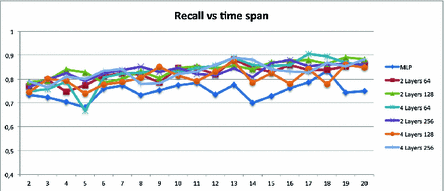
In our experiments timespans 2 to 20 samples long were used to ascertain the importance of using longer sequences to have better results. The \(F_{1}\)-score has been chosen as reference metric as it balances precision and recall.
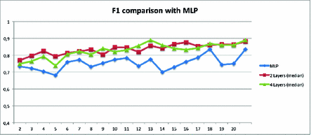
First of all, we wondered if our more complex deep networks really fared better against simpler networks: in Fig. 1 we see that the latter generally has a worse performance even at its peak at timespan = 19.
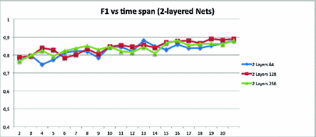
Let us first consider networks having 2 stacked, hidden LSTM layers. While sharp changes in the \(F_1\) score can be detected as the time span increases, an increasing trend may be recognized in the network having 128 neurons per LSTM layer as you use longer sequences, so we can deem it the best configuration in this subset (Fig. 2).
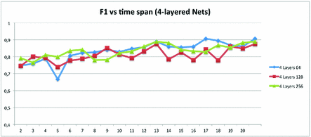
Using 4 hidden layers sharp changes in the \(F_1\) score are still present, and the same tendency evaluation we applied before can suggest the use of 64 neurons, but the increase in F1 slows down as sequences longer than 15 frames are used (Fig. 3).
Besides, having enough hidden layers to employ, choosing the right number of neurons per layer is crucial to balance feature expressiveness and training time. Considering precision and recall curves might offer some advice in this discernment.
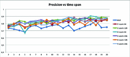
Considering precision alone as we have done in Fig. 4, we see that there is not a distinctive trend that can guide us towards the choice of a given number of frames; we can only exclude the configuration of 4 layers with 64 and 128 neurons each, that is able to fare marginally better than the MLP.
The trend of recall, as shown in Fig. 5 is very similar to precision: this may indicate either a well-balanced dataset, or the need of improvements in either feature extraction or regularization.
Both deep networks have better performance than the multilayer perceptron. On average, 2-layered Deep Networks have better precision and recall than 4-layered networks, and this reflects on the average F1 Score. As far as the accuracy is concerned they are a mostly even match.
For both deep networks the value of sigma, showing the spreading of the values across the average, is low, indicating a stable set of values near the average.
Anyway, if we take into account the very tiny differences between the shape of these curves, it seems that using 2 layers having 128 neurons each is the best course of action.
Taking into account both the metrics and the training time the 2-layered network must be preferred. The proposed system outperforms an analogous system based on a probabilistic model that is tuned with evaluation of the principal component analysis [19]. The accuracy is comparable but the F1 measure shows the neural system to be more robust (Table 1).
4 Conclusions
Within the framework of ambient intelligence, we have presented an approach to classify human indoor actions using deep neural network. We have shown that the use of networks having several stacked LSTM hidden layer have a good performance in classifying both short and long sequences of frames. To find an amenable number of hidden layers and neurons per layer a set of experiments have been carried on comparing different metrics varying the geometry the neural network.
Possible future works include:
-
the use of different, richer datasets;
-
the enrichment of the current dataset;
-
a broader experimentation with different types of hidden layers and activation functions.
References
Augello, A., Ortolani, M., Re, G.L., Gaglio, S.: Sensor mining for user behavior profiling in intelligent environments. In: Pallotta, V., Soro, A., Vargiu, E. (eds.) Advances in Distributed Agent-Based Retrieval Tools, pp. 143–158. Springer, Heidelberg (2011). doi:10.1007/978-3-642-21384-7_10
Baccouche, M., Mamalet, F., Wolf, C., Garcia, C., Baskurt, A.: Sequential deep learning for human action recognition. In: Salah, A.A., Lepri, B. (eds.) HBU 2011. LNCS, vol. 7065, pp. 29–39. Springer, Heidelberg (2011). doi:10.1007/978-3-642-25446-8_4
Bengio, Y., Courville, A., Vincent, P.: Representation learning: a review and new perspectives. IEEE Trans. Pattern Anal. Mach. Intell. 35(8), 1798–1828 (2013)
Castillo, J.C., Carneiro, D., Serrano-Cuerda, J., Novais, P., Fernández-Caballero, A., Neves, J.: A multi-modal approach for activity classification and fall detection. Int. J. Syst. Sci. 45(4), 810–824 (2014)
Cook, D.J., Augusto, J.C., Jakkula, V.R.: Ambient intelligence: technologies, applications, and opportunities. Pervasive Mob. Comput. 5(4), 277–298 (2009)
Donahue, J., Hendricks, L.A., Guadarrama, S., Rohrbach, M., Venugopalan, S., Saenko, K., Darrell, T.: Long-term recurrent convolutional networks for visual recognition and description. CoRR abs/1411.4389 (2014). http://arxiv.org/abs/1411.4389
Filippo, V., Agnese, A., Umberto, M., Vincenzo, B., Salvatore, G.: Classification of indoor actions through deep neural networks. In: 2016 International Conference on Signal-Image Technology & Internet-Based Systems (SITIS). IEEE (2016)
Graves, A.: Supervised Sequence Labelling with Recurrent Neural Networks. Studies in Computational Intelligence, vol. 385. Springer, Heidelberg (2012). doi:10.1007/978-3-642-24797-2
Hochreiter, S., Schmidhuber, J.: Long short-term memory. Neural Comput. 9(8), 1735–1780 (1997)
Krishnan, K., Prabhu, N., Babu, R.V.: ARRNET: action recognition through recurrent neural networks. In: 2016 International Conference on Signal Processing and Communications (SPCOM), pp. 1–5, June 2016
Krishnan, N.C., Cook, D.J.: Activity recognition on streaming sensor data. Pervasive Mob. Comput. Part B 10, 138–154 (2014)
Kyriazakos, S., Mihaylov, M., Anggorojati, B., Mihovska, A., Craciunescu, R., Fratu, O., Prasad, R.: eWALL: an intelligent caring home environment offering personalized context-aware applications based on advanced sensing. Wirel. Pers. Commun. 87(3), 1093–1111 (2016)
LeCun, Y., Bengio, Y., Hinton, G.: Deep learning. Nature 521(7553), 436–444 (2015)
Lima, W.S., Souto, E., Rocha, T., Pazzi, R.W., Pramudianto, F.: User activity recognition for energy saving in smart home environment. In: 2015 IEEE Symposium on Computers and Communication (ISCC), pp. 751–757. IEEE (2015)
Lowe, S.A., ÓLaighin, G.: Monitoring human health behaviour in one’s living environment: a technological review. Med. Eng. Phys. 36(2), 147–168 (2014)
Pascanu, R., Gülçehre, Ç., Cho, K., Bengio, Y.: How to construct deep recurrent neural networks. CoRR abs/1312.6026 (2013). http://arxiv.org/abs/1312.6026
Remagnino, P., Foresti, G.L.: Ambient intelligence: a new multidisciplinary paradigm. IEEE Trans. Syst. Man Cybern. Part A Syst. Hum. 35(1), 1–6 (2005)
Twomey, N., Diethe, T., Kull, M., Song, H., Camplani, M., Hannuna, S., Fafoutis, X., Zhu, N., Woznowski, P., Flach, P., Craddock, I.: The SPHERE challenge: activity recognition with multimodal sensor data. arXiv preprint arXiv:1603.00797 (2016)
Maniscalco, U., Pilato, G., Vella, F.: Detection of indoor actions through probabilistic induction model. In: De Pietro, G., Gallo, L., Howlett, R.J., Jain, L.C. (eds.) KES-IIMSS 2017. SIST, vol. 76, pp. 129–138. Springer, Cham (2018). doi:10.1007/978-3-319-59480-4_14
Vella, F., Infantino, I., Scardino, G.: Person identification through entropy oriented mean shift clustering of human gaze patterns. Multimedia Tools Appl. 76(2), 1–25 (2016)
Author information
Authors and Affiliations
Corresponding author
Editor information
Editors and Affiliations
Rights and permissions
Copyright information
© 2017 Springer International Publishing AG
About this paper
Cite this paper
Cipolla, E., Infantino, I., Maniscalco, U., Pilato, G., Vella, F. (2017). Indoor Actions Classification Through Long Short Term Memory Neural Networks. In: Battiato, S., Gallo, G., Schettini, R., Stanco, F. (eds) Image Analysis and Processing - ICIAP 2017 . ICIAP 2017. Lecture Notes in Computer Science(), vol 10484. Springer, Cham. https://doi.org/10.1007/978-3-319-68560-1_39
Download citation
DOI: https://doi.org/10.1007/978-3-319-68560-1_39
Published:
Publisher Name: Springer, Cham
Print ISBN: 978-3-319-68559-5
Online ISBN: 978-3-319-68560-1
eBook Packages: Computer ScienceComputer Science (R0)


