From Selective IBE to Full IBE and Selective HIBE

Abstract

Starting with any selectively secure identity-based encryption (IBE) scheme, we give generic constructions of fully secure IBE and selectively secure hierarchical IBE (HIBE) schemes. Our HIBE scheme allows for delegation arbitrarily many times.

Research supported in part from AFOSR YIP Award, DARPA/ARL SAFEWARE Award W911NF15C0210, AFOSR Award FA9550-15-1-0274, NSF CRII Award 1464397, and research grants by the Okawa Foundation, Visa Inc., and Center for Long-Term Cybersecurity (CLTC, UC Berkeley). The views expressed are those of the author and do not reflect the official policy or position of the funding agencies.

1 Introduction

Identity-based encryption schemes [Sha84, Coc01, BF01] (IBE) are public key encryption schemes [DH76, RSA78] for which arbitrary strings can serve as valid public keys, given short public parameters. Additionally, in such a system, given the master secret key corresponding to the public parameters, one can efficiently compute secret keys corresponding to any string $\mathsf {id}$. A popular use case for this type of encryption is certificate management for encrypted email: A sender Alice can send an encrypted email to Bob at bob@iacr.org by just using the string “bob@iacr.org” and the public parameters to encrypt the message. Bob can decrypt the email using a secret-key corresponding to “bob@iacr.org” which he can obtain from the setup authority that holds the master secret key corresponding to the public parameters.

Two main security notions for IBE have been considered in the literature—selective security and full security. In the selective security experiment of identity-based encryption [CHK04], the adversary is allowed to first choose a challenge identity and may then obtain the public parameters and the identity secret keys for identities different from the challenge identity. The adversary’s goal is to distinguish messages encrypted under the challenge identity, for which he is not allowed to obtain a secret key. On the other hand, in the fully secure notion [BF01], the (adversarial) choice of the challenge identity may depend arbitrarily on the public parameters. That is, the adversary may choose the challenge identity after seeing the public parameters and any number of identity secret keys of its choice. It is straightforward to see that any scheme that features full security is also selectively secure. On the other hand, example IBE schemes that are selectively secure but trivially insecure in the full security sense can be constructed without significant effort.

The first IBE scheme was realized by Boneh and Franklin [BF01] based on bilinear maps. Soon after, Cocks [Coc01] provided the first IBE scheme based on quadratic residuocity assumption. However, the security of these constructions was argued in the random oracle model [BR93]. Subsequently, substantial effort was devoted to realizing IBE schemes without random oracles. The first constructions of IBE without random oracles were only proved to be selectively secure [CHK04, BB04a] and achieving full security for IBE without the random oracle heuristic required significant research effort. In particular, the first IBE scheme meeting the full security definition in the standard model were constructed by Boneh and Boyen [BB04b] and Waters [Wat05] using bilinear maps. Later, several other IBE schemes based on the learning with errors assumption [Reg05] were proposed [GPV08, AB09, CHKP10, ABB10a]. Very recently, constructions based on the security of the Diffie-Hellman Assumption and Factoring have also be obtained [DG17].

Basic IBE does not support the capability of delegating the power to issue identity secret keys. This property is captured by the notion of hierarchical identity-based encryption (HIBE) [HL02, GS02]. In a HIBE scheme, the owner of a master secret key can issue delegated master secret keys that enable generating identity secret keys for identities that start with a certain prefix. For instance, Alice may use a delegated master secret key to issue an identity secret key to her secretary for the identity “alice@iacr.org $\Vert$ 05-24-2017”, allowing the secretary to decrypt all her emails received on this day. While HIBE trivially implies IBE, the converse question has not been resolved yet. Abdalla, Fiore and Lyubashevsky [AFL12] provided constructions of fully secure HIBE from selective-pattern-secure wildcarded identity-based encryption (WIBE) schemes [ACD+06] and a construction of WIBE from HIBE schemes fulfilling the stronger notion of security under correlated randomness. Substantial effort has been devoted to realizing HIBE schemes based on specific assumptions [GS02, BB04b, BBG05, GH09, LW10, CHKP10, ABB10b, DG17].

The question whether selectively secure IBE generically implies fully secure IBE or HIBE remains open hitherto.

1.1 Our Results

In this work, we provide a generalization of the framework developed in [DG17]. Specifically, we replace the primitive chameleon encryption (or, chameleon hash function with encryption) from [DG17] with a weaker primitive which we call one-time signatures with encryption (OTSE). We show that this weaker primitive¹ also suffices for realizing fully secure IBE and selectively secure HIBE building on the techniques of [DG17]. We show that OTSE can be realized from chameleon encryption, which, as shown in [DG17], can be based on the Computational Diffie-Hellman Assumption.

In the context of [DG17], OTSE can be seen as an additional layer of abstraction that further modularizes the IBE construction of [DG17]. More concretely, when plugging the construction of OTSE from chameleon encryption (Sect. 4) into the construction of HIBE from OTSE (Sect. 7), one obtains precisely the HIBE construction of [DG17]².

The new insight in this work is that OTSE, unlike chameleon encryption, can be realized generically from any selectively secure IBE scheme. As a consequence, it follows that both fully secure IBE and selectively secure HIBE can also be constructed generically from any selectively secure IBE scheme. Prior works on broadening the assumptions sufficient for IBE and HIBE have focused on first realizing selectively secure IBE. Significant subsequent research has typically been needed for realizing fully secure IBE and HIBE. Having a generic construction immediately gives improvements over previously known results and makes it easier to achieve improvements in the future. For example, using the new IBE construction of Gaborit et al. [GHPT17] we obtain a new construction of HIBE from the rank-metric problem. As another example, we obtain a construction of selectively secure HIBE from LWE with compact public parameters, i.e. a HIBE scheme where the size of the public parameters does not depend on a maximum hierarchy depth [CHKP10, ABB10b].

1.2 Technical Outline

The results in this work build on a recent work of the authors [DG17], which provides an IBE scheme in groups without pairings. In particular, we will employ the tree-based bootstrapping technique of [DG17], which itself was inspired by the tree-based construction of Laconic Oblivious Transfer, a primitive recently introduced by Cho et al. [CDG+17]. Below, we start by recalling [DG17] and expand on how we generalize that technique to obtain our results.

Challenge in Realizing the IBE Schemes. The key challenge in realizing IBE schemes is the need to “somehow compress” public keys corresponding to all possible identities (which could be exponentially many) into small public parameters. Typically, IBE schemes resolve this challenge by generating the “identity specific” public keys in a correlated manner. Since these public keys are correlated they can all be described with succinct public parameters. However, this seems hard to do when relying on an assumption such as the Diffie-Hellman Assumption. Recently, [DG17] introduced new techniques for compressing multiple uncorrelated public keys into small public parameters allowing for a construction based on the Diffie-Hellman Assumption. Below we start by describing the notion of chameleon encryption and how the IBE scheme of [DG17] uses it.

Chameleon Encryption at a High Level. At the heart of the [DG17] construction is a new chameleon hash function [KR98] with some additional encryption and decryption functionality. A (keyed) chameleon hash function $\mathsf {H}_\mathsf {k}: \{0,1\}^n \times \{0,1\}^\lambda \rightarrow \{0,1\}^\lambda$ on input an n-bit string $\mathsf {x}$ (for $n > \lambda$) and random coins $r\in \{0,1\}^\lambda$ outputs a $\lambda$-bit string. The keyed hash function is such that a trapdoor $\mathsf {t}$ associated to $\mathsf {k}$ can be used to find collisions. In particular, given a trapdoor $\mathsf {t}$ for $\mathsf {k}$, a pair of input and random coins $(\mathsf {x},r)$ and an alternative preimage $\mathsf {x}'$ it is easy to compute coins $r'$ such that $\mathsf {H}_\mathsf {k}(\mathsf {x};r) = \mathsf {H}_\mathsf {k}(\mathsf {x}',r')$. Additionally, we require the following encryption and decryption procedures. The encryption function outputs a ciphertext c such that decryption yields the original message m back as long as

$$\mathsf {h}= \mathsf {H}_{\mathsf {k}}(\mathsf {x};r) \text { and } \mathsf {x}_i = b,$$

where $(\mathsf {h},i,b)$ are the values used in the generation of the ciphertext $\mathsf {ct}$. In other words, the decryptor can use the knowledge of the preimage of $\mathsf {h}$ as the secret key to decrypt $\mathsf {m}$ as long as the $i^{th}$ bit of the preimage it can supply is equal to the value b chosen at the time of encryption. Roughly, the security requirement of chameleon encryption is that

$$\begin{aligned} \{\mathsf {k}, \mathsf {x}, r, \mathsf {Enc}(\mathsf {k}, (\mathsf {h}, i, 1-\mathsf {x}_i), 0)\} {\mathop {\approx }\limits ^{c}}\{\mathsf {k}, \mathsf {x}, r, \mathsf {Enc}(\mathsf {k}, (\mathsf {h}, i, 1-\mathsf {x}_i), 1)\}, \end{aligned}$$

where ${\mathop {\approx }\limits ^{c}}$ denotes computational indistinguishability. In other words, if an adversary is given a preimage $\mathsf {x}$ of the hash value $\mathsf {h}$, but the $i^{th}$ bit of $\mathsf {h}$ is different from the value b used during encryption, then ciphertext indistinguishability holds.

Realization of Chameleon Encryption. [DG17] provide the following very natural realization of the Chameleon Encryption under the DDH assumption. Given a group $\mathbb {G}$ of prime order p with a generator g, the hash function $\mathsf {H}$ is computed as follows:

$$\begin{aligned} \mathsf {H}_\mathsf {k}(\mathsf {x};r) = g^r\prod _{j\in [n]} g_{j,\mathsf {x}_j}, \end{aligned}$$

where the key $\mathsf {k}= (g, \{g_{j,0}, g_{j,1}\}_{j \in [n]})$, $r \in \mathbb {Z}_p$ and $\mathsf {x}_j$ is the $j^{th}$ bit of $\mathsf {x}\in \{0,1\} ^n$.

Corresponding to this chameleon hash function the encryption procedure $\mathsf {Enc}(\mathsf {k}, (\mathsf {h},i,b),\mathsf {m})$ proceeds as follows. Sample a random value and output the ciphertext $\mathsf {ct}=(e, c, c', \{c_{j,0},c_{j,1}\}_{j \in [n] \backslash \{ i \}})$, where $c := g^\rho$, $c' := \mathsf {h}^\rho$, $\forall j \in [n]\backslash \{i\},~c_{j,0} :=g_{j,0}^\rho ,~ c_{j,1}:=g_{j,1}^\rho ,$ and $e := \mathsf {m}\oplus g^\rho _{i,b}.$ It is easy to see that if $\mathsf {x}_i = b$, then decryption $\mathsf {Dec}(\mathsf {ct}, (\mathsf {x},r))$ can be performed by computing

$$\begin{aligned} e\oplus \frac{c'}{c^r\prod _{j \in [n]\backslash \{i\}} c_{j,\mathsf {x}_j}}. \end{aligned}$$

However, if $\mathsf {x}_i \ne b$ then the decryptor has access to the value $g_{i,x_i}^\rho$ but not $g_{i,b}^\rho$, and this prevents him from learning the message $\mathsf {m}$. This observation can be formalized as a security proof based on the DDH assumption³ and we refer the reader to [DG17] for the details.

From Chameleon Encryption to Identity-Based Encryption [DG17]. As mentioned earlier, [DG17] provide a technique for compressing uncorrelated public keys. [DG17] achieve this compression using the above-mentioned hash function in a Merkle-hash-tree fashion. In particular, the public parameters of the [DG17] IBE scheme consist of the key of the hash function and the root of the Merkle-hash-tree hashing the public keys of all the parties. Note that the number of identities is too large (specifically it is exponential) to efficiently hash all the identity-specific public keys into short public parameters. Instead [DG17] use the chameleon property of the hash function to generate the tree top-down rather than bottom-up (as is typically done in a Merkle-tree hashing). We skip the details of this top-down Merkle tree generation and refer to [DG17].

A secret key for an identity $\mathsf {id}$ in the [DG17] scheme consists of the hash-values along the root-to-leaf path corresponding to the leaf node $\mathsf {id}$ in the Merkle-hash-tree. We also include the siblings of the hash-values provided and the random coins used. Moreover, it includes the secret key corresponding to the public key at the leaf-node $\mathsf {id}$.

Encryption and decryption are based on the following idea. Let $\{ Y_{j,0}, Y_{j,1} \}_{j \in [n]}$ be 2n labels. Given a hash-value $\mathsf {h}$, an encryptor can compute the ciphertexts ${c}_{j,b} :=\mathsf {Enc}(\mathsf {k},(\mathsf {h},j,b),Y_{j,b})$ for $j = 1,\dots ,n$ and $b \in \{0,1\}$. Given the ciphertexts $\{{c}_{j,0}, {c}_{j,1} \}_{j \in [n]}$, a decryptor in possession of a message $\mathsf {x}$ and coins $r$ with $\mathsf {H}_\mathsf {k}(\mathsf {x};r) = \mathsf {h}$ can now decrypt the ciphertexts $\{ {c}_{j,\mathsf {x}_j} \}_{j \in [n]}$ and obtain the labels $Y_{j,\mathsf {x}_j} :=\mathsf {Dec}(\mathsf {k},(\mathsf {x},r),{c}_{j,\mathsf {x}_j})$ for $j = 1,\dots ,n$. Due to the security of the chameleon encryption scheme, the decryptor will learn nothing about the labels $\{ Y_{j,1 - \mathsf {x}_j}\}_{j \in [n]}$.

This technique can be combined with a projective garbling scheme to help an encryptor provide a value $\mathsf {C} (\mathsf {x})$ to the decryptor, where $\mathsf {C}$ is an arbitrary circuit that knows some additional secrets chosen by the encryptor. The key point here being that the encryptor does not need to know the value $\mathsf {x}$, but only a hash-value $\mathsf {h}= \mathsf {H}_\mathsf {k}(\mathsf {x};r)$. The encryptor garbles the circuit $\mathsf {C}$ and obtains a garbled circuit $\tilde{\mathsf {C}}$ and labels $\{ Y_{j,0}, Y_{j,1} \}$ for the input-wires of $\mathsf {C}$. Encrypting the labels in the above fashion, (i.e. computing ${c}_{j,b} :=\mathsf {Enc}(\mathsf {k},(\mathsf {h},j + \mathsf {id}_i \cdot \lambda ,b),Y_{j,b})$), we obtain a ciphertext $\mathsf {ct}:=(\tilde{\mathsf {C}}, \{ {c}_{j,0}, {c}_{j,1} \}_{j \in [n]})$.

Given such a ciphertext, by the above a decryptor can obtain the labels $\{ Y_{j,\mathsf {x}_j} \}_{j \in [n]}$ corresponding to the input $\mathsf {x}$ and evaluate the garbled circuit $\tilde{\mathsf {C}}$ to obtain $\mathsf {C} (\mathsf {x})$. By the security property of the garbling scheme and the discussion above the decryptor will learn nothing about the circuit $\mathsf {C}$ but the output-value $\mathsf {C} (\mathsf {x})$.

The encryption procedure of the IBE scheme provided in [DG17] uses this technique as follows. It computes a sequence of garbled circuits $\tilde{\mathsf {Q}}^{(1)},\dots ,\tilde{\mathsf {Q}}^{(n)}$, where the circuit $\mathsf {Q} ^{(i)}$ takes as input a hash-value $\mathsf {h}$, and returns chameleon encryptions $\{{c}_{j,0}, {c}_{j,1} \}_{j \in [n]}$ of the input-labels $\{ Y^{(i+1)}_{j,0}, Y^{(i+1)}_{j,1}\}_{j \in [n]}$ of $\mathsf {Q} ^{(i+1)}$, where ${c}_{j,b} :=\mathsf {Enc}(\mathsf {k},(\mathsf {h},j+ \mathsf {id}_i \cdot \lambda ,b),Y^{(i+1)}_{j,b})$. The last garbled circuit $\mathsf {Q} ^{(n)}$ in this sequence outputs chameleon encryptions of the labels $\{ T_{j,0}, T_{j,1}\}_{j \in [n]}$ of a garbled circuit $\mathsf {T}$, where the circuit $\mathsf {T}$ takes as input a public key $\mathsf {pk}$ of a standard public key encryption scheme $(\mathsf {KG},\mathsf {E},\mathsf {D})$ and outputs and encryption $\mathsf {E}(\mathsf {pk},\mathsf {m})$ of the message $\mathsf {m}$. The IBE ciphertext consists of the chameleon encryptions $\{{c}^{(1)}_{j,0}, {c}^{(1)}_{j,1} \}_{j \in [n]}$ of the input labels of the first garbled circuit $\tilde{\mathsf {Q}}^{(1)}$, the garbled circuits $\tilde{\mathsf {Q}}^{(1)},\dots ,\tilde{\mathsf {Q}}^{(n)}$ and the garbled circuit $\tilde{\mathsf {T}}$.

The decryptor, who is in possession of the siblings along the root-to-leaf path for identity $\mathsf {id}$, can now traverse the tree as follows. He starts by decrypting $\{{c}^{(1)}_{j,0}, {c}^{(1)}_{j,1} \}_{j \in [n]}$ to the labels corresponding the first pair of siblings, evaluating the garbled circuit $\tilde{\mathsf {Q}}^{(1)}$ on this input and thus obtain chameleon encryptions $\{{c}^{(2)}_{j,0}, {c}^{(2)}_{j,1} \}_{j \in [n]}$ of the labels of the next garbled circuit $\tilde{\mathsf {Q}}^{(2)}$. Repeating this process, the decryptor will eventually be able to evaluate the last garbled circuit $\tilde{\mathsf {T}}$ and obtain $\mathsf {E}(\mathsf {pk}_\mathsf {id},\mathsf {m})$, an encryption of the message $\mathsf {m}$ under the leaf-public-key $\mathsf {pk}_\mathsf {id}$. Now this ciphertext can be decrypted using the corresponding leaf-secret-key $\mathsf {sk}_\mathsf {id}$.

Stated differently, the encryptor uses the garbled circuits $\tilde{\mathsf {Q}}^{(1)},\dots ,\tilde{\mathsf {Q}}^{(n)}$ to help the decryptor traverse the tree to the leaf corresponding to the identity $\mathsf {id}$ and obtain an encryption of $\mathsf {m}$ under the leaf-public key $\mathsf {pk}_\mathsf {id}$ (which is not know to the encryptor).

Security of this scheme follows, as sketched above, from the security of the chameleon encryption scheme, the garbling scheme and the security of the public key encryption scheme $(\mathsf {KG},\mathsf {E},\mathsf {D})$.

Connection to a Special Signature Scheme. It is well-known that IBE implies a signature scheme—specifically, by interpreting the secret key for an identity $\mathsf {id}$ as the signature on the message $\mathsf {id}$. The starting point of our work is the observation that the [DG17] IBE scheme has similarities with the construction of a signature scheme from a one-time signature scheme [Lam79, NY89]. In particular, the chameleon hash function mimics the role of a one-time signature scheme which can then be used to obtain a signature scheme similar to the IBE scheme of [DG17]. Based on this intuition we next define a new primitive which we call one-time signature with encryption which is very similar to (though weaker than) chameleon encryption. Construction of one-time signature with encryption from chameleon encryption is provided in Sect. 4.

One-Time Signatures with Encryption. A one-time signature scheme [Lam79, NY89] is a signature scheme for which security only holds if a signing key is used at most once. In more detail, a one-time signature scheme consists of three algorithms $(\mathsf {SGen}, \mathsf {SSign}, \mathsf {Verify})$, where $\mathsf {SGen}$ produces a pair $(\mathsf {vk},\mathsf {sk})$ of verification and signing keys, $\mathsf {SSign}$ takes a signing key $\mathsf {sk}$ and a message $\mathsf {x}$ and produces a signature $\sigma$, and $\mathsf {Verify}$ takes a message-signature pair $(\mathsf {x},\sigma )$ and checks if $\sigma$ is a valid signature for $\mathsf {x}$. One-time security means that given a verification key and a signature $\sigma$ on a message of its own choice, an efficient adversary will not be able to concoct a valid signature $\sigma '$ on a different message $\mathsf {x}'$.

As with chameleon encryption, we will supplement the notion of one-time signature schemes with an additional encryption functionality. More specifically, we require additional encryption and decryption algorithms $\mathsf {SEnc}$ and $\mathsf {SDec}$ with the following properties. $\mathsf {SEnc}$ encrypts a message $\mathsf {m}$ using parameters $(\mathsf {vk},i,b)$, i.e. a verification key , an index i and a bit b, and any message signature pair satisfying “$\mathsf {Verify} (\mathsf {vk},\mathsf {x},\sigma ) = 1$ and $\mathsf {x}_i = b$” can be used with $\mathsf {SDec}$ to decrypt the plaintext $\mathsf {m}$. In terms of security, we require that given a signature $\sigma$ on a selectively chosen message $\mathsf {x}$, it is infeasible to distinguish encryptions for which the bit b is set to $1-\mathsf {x}_i$, i.e. $\mathsf {SEnc} ((\mathsf {vk},i,1 - \mathsf {x}_i),\mathsf {m} _0)$ and $\mathsf {SEnc} ((\mathsf {vk},i,1 - \mathsf {x}_i),\mathsf {m} _1)$ are indistinguishable for any pair of messages $\mathsf {m} _0,\mathsf {m} _1$.

Finally, we will have the additional requirement that the verification keys are succinct, i.e. the size of the verification keys does not depend on the length of the messages that can be signed.

In the following, we will omit the requirement of a verification algorithm $\mathsf {Verify}$, as such an algorithm is implied by the $\mathsf {SEnc}$ and $\mathsf {SDec}$ algorithms⁴.

Moreover, we remark that in the actual definition of OTSE in Sect. 3, we introduce additional public parameters $\mathsf {pp}$ that will be used to sample verification and signing keys.

In Sect. 4, we will provide a direct construction of an OTSE scheme from chameleon encryption [DG17]. We remark that the techniques used in this construction appear in the HIBE-from-chameleon-encryption construction of [DG17].

We will now sketch a construction of an OTSE scheme from any selectively secure IBE scheme. Assume henceforth that $(\mathsf {Setup},\mathsf {KeyGen},\mathsf {Encrypt},\mathsf {Decrypt})$ is a selectively secure IBE scheme. We will construct an OTSE scheme $(\mathsf {SGen},\mathsf {SSign},\mathsf {SDec})$ as follows. $\mathsf {SGen}$ runs the $\mathsf {Setup}$ algorithm and sets $\mathsf {vk} :=\mathsf {mpk}$ and $\mathsf {sk}:=\mathsf {msk}$, i.e. the master public key $\mathsf {mpk}$ will serve as verification key and the master secret key $\mathsf {msk}$ will serve as signing key $\mathsf {sk}$. To sign a message , compute identity secret keys for the identities for . Here, $\mathsf {x}_j$ is the j-th bit of is the string concatenation operator and is a bits representation of the index . Thus, a signature $\sigma$ of $\mathsf {x}$ is computed by

$$ \sigma = \mathsf {SSign} (\mathsf {sk},\mathsf {x}) :=\{ \mathsf {KeyGen} (\mathsf {msk},\mathsf {x}_j \Vert \mathsf {bin}(j)) \}_{j \in [n]}. $$

It can be checked that this is a correct and secure one-time signature scheme. The encryption and decryption algorithms $\mathsf {SEnc}$ and $\mathsf {SDec}$ are obtained from the $\mathsf {Encrypt}$ and $\mathsf {Decrypt}$ algorithms of the IBE scheme. Namely, to encrypt a plaintext $\mathsf {m}$ using $\mathsf {vk} = \mathsf {mpk},i,b$, compute the ciphertext

$$ {c}= \mathsf {SEnc} ((\mathsf {vk},i,b),\mathsf {m}) :=\mathsf {Encrypt} (\mathsf {mpk},b \Vert \mathsf {bin}(i),\mathsf {m}), $$

i.e. we encrypt $\mathsf {m}$ to the identity . Decryption using a signature $\sigma$ on a message $\mathsf {x}$ is performed by computing

$$ \mathsf {m} = \mathsf {SDec} ((\sigma ,\mathsf {x}),{c}) :=\mathsf {Decrypt} (\mathsf {sk}_{\mathsf {x}_i \Vert \mathsf {bin}(i)},{c}), $$

which succeeds if . The succinctness requirement is fulfilled, as the size of the verification keys (which are master public keys) depends only (polynomially) on the security parameter, but not on the actual number of identities.

Security can be based on the selective security of the IBE scheme by noting that if the i-th bit of the message $\mathsf {x}$ for which a signature has been issued is different from b, then the identity secret key corresponding to the identity is not contained in $\sigma$ and we can use the selective security of the IBE scheme.

Realizing Fully Secure IBE. We will now show how an OTSE scheme can be bootstrapped into a fully secure IBE scheme. As mentioned before, we will use the tree based approach of the authors [DG17]. For the sake of simplicity, we will describe a stateful scheme, i.e. the key-generation algorithm keeps a state listing the identity secret keys that have been issued so far. The actual scheme, described in Sect. 6, will be a stateless version of this scheme, which can be obtained via pseudorandom functions.

We will now describe how identity secret keys are generated. The key generation algorithm of our scheme can be seen as an instance of the tree-based construction of a signature scheme from one-time signatures and universal one-way hash functions [NY89]. In fact, our OTSE scheme serves as one-time signature scheme with short verification keys in the construction of [NY89]. In [NY89], one-time signature scheme with short verification keys are used implicitly via a combination of one-time signatures and universal one-way hash functions.

Assume that identities are of length n and that we have a binary tree of depth n. Nodes in this tree are labelled by binary strings $\mathsf {v}$ that correspond to the path to this node from the root, and the root itself is labelled by the empty string .

We will place public keys of a standard $\mathsf {IND}^{\mathsf {CPA}}$-secure encryption scheme $(\mathsf {KG},\mathsf {E},\mathsf {D})$ into the leaf-nodes $\mathsf {v}$ of the tree and a verification key of the OTSE scheme into every node $\mathsf {v}$. The nodes are connected in the following manner. If $\mathsf {v}$ is a node with two children and , we will concatenate the keys and and sign them with the signing key (corresponding to the verification key ), i.e. define and compute

$$ \sigma _{\mathsf {v}} :=\mathsf {SSign} (\mathsf {sk}_\mathsf {v},\mathsf {x}). $$

If $\mathsf {v}$ is a leaf-node, compute

$$ \sigma _{\mathsf {v}} :=\mathsf {SSign} (\mathsf {sk}_\mathsf {v},\mathsf {lpk} _\mathsf {v}), $$

after padding $\mathsf {lpk} _\mathsf {v}$ to the appropriate length.

The master public key $\mathsf {mpk}$ of our scheme consist of the verification key at the root node $\mathsf {v}_0$. The identity secret key for a root-to-leaf path $\mathsf {v} _0,\dots ,\mathsf {v} _n$ consists of the root verification key , the (i.e. the verification keys for the siblings along the path), the signatures $\sigma _{\mathsf {v} _0},\dots ,\sigma _{\mathsf {v} _n}$, and the leaf public and secrets keys $\mathsf {lpk} _{\mathsf {v} _n}$ and $\mathsf {lsk} _{\mathsf {v} _n}$.

We can think of the entire information in the identity secret key as public information, except the leaf secret key $\mathsf {lsk} _{\mathsf {v} _n}$. That is, from a security perspective they could as well be made publicly accessible (they are not, due to the succinctness constraint of the master public key).

Encryption and Decryption. We will now describe how a plaintext is encrypted to an identity $\mathsf {id}$ and how it is decrypted using the corresponding identity secret key $\mathsf {sk}_\mathsf {id}$. The basic idea is, as in [DG17], that the encryptor delegates encryption of the plaintext $\mathsf {m}$ to the decryptor. More specifically, while the encryptor only knows the root verification key, the decryptor is in possession of all verification keys and signatures along the root-to-leaf path for the identity.

This delegation task will be achieved using garbled circuits along with the OTSE scheme. The goal of this delegation task is to provide a garbled circuit $\tilde{\mathsf {T}}$ with the leaf public key $\mathsf {lpk} _{\mathsf {id}}$ for the identity $\mathsf {id}$. To ensure that the proper leaf public key is provided to $\tilde{\mathsf {T}}$, a sequence of garbled circuits $\tilde{\mathsf {Q}}^{(0)},\dots ,\tilde{\mathsf {Q}}^{(n)}$ is used to traverse the tree from the root to the leaf $\mathsf {id}$.

First consider a tree that consists of one single leaf-node $\mathsf {v}$, i.e. in this case there is just one leaf public key $\mathsf {lpk} _\mathsf {v}$ and one verification key $\mathsf {vk}_{\mathsf {v}}$. The signature $\sigma$ is given by

$$ \sigma :=\mathsf {SSign} (\mathsf {sk}_{\mathsf {v}},\mathsf {lpk} _\mathsf {v}) $$

The encryptor wants to compute an encryption of a plaintext $\mathsf {m}$ under $\mathsf {lpk} _\mathsf {v}$, while only in possession of the verification key $\mathsf {vk}_\mathsf {v}$. It will do so using a garbled circuit $\tilde{\mathsf {T}}$. The garbled circuit $\tilde{\mathsf {T}}$ has the plaintext $\mathsf {m}$ hardwired, takes as input a local public key $\mathsf {lpk}$ and outputs an encryption of the plaintext $\mathsf {m}$ under $\mathsf {lpk}$, i.e. $\mathsf {E}(\mathsf {lpk},\mathsf {m})$. Let $\{T_{j,0},T_{j,1}\}_{j \in [\ell ]}$ be the set of input labels for the garbled circuit $\tilde{\mathsf {T}}$. In this basic case, the ciphertext consists of the garbled circuit $\tilde{\mathsf {T}}$ and encryptions of the labels $\{T_{j,0},T_{j,1}\}_{j \in [\ell ]}$ under the OTSE scheme. More specifically, for all $j \in [\ell ]$ and $b \in \{0,1\}$ the encryptor computes ${c}_{j,b} :=\mathsf {SEnc} ((\mathsf {vk}_\mathsf {v},j,b),T_{j,b})$ and sets the ciphertext to $\mathsf {ct}:=(\tilde{\mathsf {T}},\{ {c}_{j,b} \}_{j,b})$.

To decrypt such a ciphertext $\mathsf {ct}$ given $\mathsf {lsk} _\mathsf {v}$, $\mathsf {lpk} _\mathsf {v}$ and a signature $\sigma _\mathsf {v}$ of $\mathsf {lpk} _\mathsf {v}$ we proceed as follows. First, the decryptor recovers the labels $\{ T_{j,(\mathsf {lpk} _\mathsf {v})_j} \}_j$ (where $(\mathsf {lpk} _\mathsf {v})_j$ is the j-th bit of $\mathsf {lpk} _\mathsf {v}$) by computing

$$ T_{j,(\mathsf {lpk} _\mathsf {v})_j} :=\mathsf {SDec} ((\sigma ,\mathsf {lpk} _\mathsf {v}),{c}_{j,(\mathsf {lpk} _\mathsf {v})_j}). $$

By the correctness of the OTSE scheme it follows that these are indeed the correct labels corresponding to $\mathsf {lpk} _\mathsf {v}$. Evaluating the garbled circuit $\tilde{\mathsf {T}}$ on these labels yields an encryption $\mathsf {f} = \mathsf {E}(\mathsf {lpk} _\mathsf {v},\mathsf {m})$ of the plaintext $\mathsf {m}$. Now the secret key $\mathsf {lsk} _\mathsf {v}$ can be used to decrypt $\mathsf {f}$ to the plaintext $\mathsf {m}$.

For larger trees, the encryptor is not in possession of the verification key $\mathsf {vk}_\mathsf {v}$ of the leaf-node $\mathsf {v}$, and can therefore not compute the encryptions ${c}_{j,b} :=\mathsf {SEnc} ((\mathsf {vk}_\mathsf {v},j,b),T_{j,b})$ by herself. This task will therefore be delegated to a sequence of garbled circuits $\tilde{\mathsf {Q}}^{(0)},\dots ,\tilde{\mathsf {Q}}^{(n)}$. For $i =0,\dots ,n-1$, the garbled circuit $\tilde{\mathsf {Q}}^{(i)}$ has the bit $\mathsf {id}_{i+1}$ and the labels $\{X_{j,b} \}_{j,b}$ of the next garbled circuit $\tilde{\mathsf {Q}}^{(i+1)}$ hardwired, takes as input a verification key $\mathsf {vk}_\mathsf {v}$ and outputs $\{ {c}_{j,b} \}_{j,b}$, where ${c}_{j,b} :=\mathsf {SEnc} ((\mathsf {vk}_\mathsf {v},\mathsf {id}_{i+1} \cdot \ell + j,b),X_{j,b})$. The garbled circuit $\tilde{\mathsf {Q}}^{(n)}$ has the labels $\{T_{j,b} \}_{j,b}$ of the garbled circuit $\tilde{\mathsf {T}}$ hardwired, takes as input a verification key $\mathsf {vk}_\mathsf {v}$ and outputs $\{ {c}_{j,b} \}_{j,b}$, where ${c}_{j,b} :=\mathsf {SEnc} ((\mathsf {vk}_\mathsf {v},j,b),T_{j,b})$.

Thus, a decryptor who knows input labels for $\tilde{\mathsf {Q}}^{(i)}$ corresponding to $\mathsf {vk}_{\mathsf {v}}$ will be able to evaluate $\tilde{\mathsf {Q}}^{(i)}$ and obtain the encrypted labels $\{ {c}_{j,b} \}_{j,b}$, where ${c}_{j,b} = \mathsf {SEnc} ((\mathsf {vk}_\mathsf {v},\mathsf {id}_{i+1} \cdot \ell + j,b),X_{j,b})$. If the decryptor is in possession of the values $\mathsf {x}_\mathsf {v} = \mathsf {vk}_{\mathsf {v} _i \Vert 0} \Vert \mathsf {vk}_{\mathsf {v} _i \Vert 1}$ and a valid signature $\sigma _\mathsf {v}$ of $\mathsf {x}_\mathsf {v}$ that verifies with respect to $\mathsf {vk}_{\mathsf {v}}$, he will be able to compute

$$ X_{j,(\mathsf {vk}_{\mathsf {v} \Vert \mathsf {id}_i} )_j} :=\mathsf {SDec} ((\sigma _\mathsf {v},\mathsf {x}_\mathsf {v}),{c}_{j,(\mathsf {vk}_{\mathsf {v} \Vert \mathsf {id}_i})_j}). $$

These are the input labels of $\tilde{\mathsf {Q}}^{(i+1)}$ corresponding to the input $\mathsf {vk}_{\mathsf {v} \Vert \mathsf {id}_{i+1}}$. Consequently, the decryptor will be able to evaluate $\tilde{\mathsf {Q}}^{(i+1)}$ on input $\mathsf {vk}_{\mathsf {v} \Vert \mathsf {id}_{i+1}}$ and so forth.

Thus, in the full scheme a ciphertext $\mathsf {ct}$ consists of the input-labels of the garbled circuit $\tilde{\mathsf {Q}}^{(0)}$, the sequence of garbled circuits $\tilde{\mathsf {Q}}^{(0)},\dots ,\tilde{\mathsf {Q}}^{(n)}$ and a garbed circuit $\tilde{\mathsf {T}}$. To decrypt this ciphertext, proceed as above starting with the garbled circuit $\tilde{\mathsf {Q}}^{(0)}$ and traversing the tree to the leaf-node $\mathsf {id}$, where $\tilde{\mathsf {T}}$ can be evaluated and the plaintext $\mathsf {m}$ be recovered as above.

In the security proof, we will replace the garbled circuits with simulated garbled circuits and change the encryptions to only encrypt labels for the next verification key in the sequence of nodes. One key idea here is that the security reduction knows all the verification keys and signatures in the tree, which as mentioned above is not private but not accessible to the real encryptor due to succinctness requirements of the public parameters. See Sect. 6 for details.

Hierarchical IBE. To upgrade the above scheme into a HIBE scheme, we will associate a local public key $\mathsf {lpk} _{\mathsf {v} \mathsf {v}}$ with each node $\mathsf {v}$ of the tree, i.e. each node of the tree may serve as a leaf in the above scheme if needed. This means each node will contain a signature of the verification keys of the two child nodes and the local public key, i.e. we set $\mathsf {x} :=\mathsf {vk}_{\mathsf {v} \Vert 0} \Vert \mathsf {vk}_{\mathsf {v} \Vert 1} \Vert \mathsf {lpk} _{\mathsf {v}}$ and compute

$$ \sigma _\mathsf {v} :=\mathsf {SSign} (\mathsf {sk}_\mathsf {v},\mathsf {x}) $$

Moreover, we can make this scheme stateless using a pseudorandom function that supports the delegation of keys. In particular, the classic GGM construction [GGM86] supports delegation of PRF keys for subtrees when instantiated appropriately. We are only able to prove selective security of the obtained HIBE scheme, as in the HIBE experiment the delegation keys include PRF keys, something that was not needed to be done for the case of IBE.

2 Preliminaries

Let $\lambda$ denote the security parameter. We use the notation [n] to denote the set $\{1,\ldots ,n\}$. By PPT we mean a probabilistic polynomial time algorithm. For any set S, we use $x \xleftarrow {\$}S$ to denote that x is sampled uniformly at random from the set S.⁵ Alternatively, for any distribution D we use $x \xleftarrow {\$}D$ to denote that x is sampled from the distribution D. We use the operator $:=$ to represent assignment and $=$ to denote an equality check. For two strings $\mathsf {x}$ and , we denote the concatenation of $\mathsf {x}$ and $\mathsf {x}'$ by $\mathsf {x} \Vert \mathsf {x}'$. For an integer $j \in [n]$, let $\mathsf {bin}(j)$ be the bits representation of j.

2.1 Public Key Encryption

Definition 1 (Public Key Encryption)

A public key encryption scheme consists of three PPT algorithms $(\mathsf {KG},\mathsf {E},\mathsf {D})$ with the following syntax.

• $\mathsf {KG}(1^\lambda )$ takes as input a security parameter $1^\lambda$ and outputs a pair of public and secret keys $(\mathsf {pk},\mathsf {sk})$.

• $\mathsf {E}(\mathsf {pk},\mathsf {m})$ takes as input a public key $\mathsf {pk}$ and a plaintext $\mathsf {m}$ and outputs a ciphertext ${c}$.

• $\mathsf {D}(\mathsf {sk},{c})$ takes as input a secret key $\mathsf {sk}$ and a ciphertext ${c}$ and outputs a plaintext $\mathsf {m}$.

We require the following properties to hold.

• Completeness: For every security parameter $\lambda$ and for all messages $\mathsf {m}$, it holds that

  $$ \mathsf {D}(\mathsf {sk},\mathsf {E}(\mathsf {pk},\mathsf {m})) = \mathsf {m}, $$

  where $(\mathsf {pk},\mathsf {sk}) :=\mathsf {KG}(1^\lambda )$.

• $\mathsf {IND}^{\mathsf {CPA}}$ Security: For any PPT adversary $\mathcal {A} = (\mathcal {A} _1,\mathcal {A} _2)$, there exists a negligible function $\mathsf {negl}(\cdot )$ such that the following holds:

  $$ \Pr [\mathsf {IND}^{\mathsf {CPA}} (\mathcal {A}) = 1] \le \dfrac{1}{2} + \mathsf {negl}(\lambda ) $$

  where $\mathsf {IND}^{\mathsf {CPA}} (\mathcal {A})$ is shown in Fig. 1.

Fig. 1.

The $\mathsf {IND}^{\mathsf {CPA}} (\mathcal {A})$ experiment

This notion easily extends to multiple challenge-ciphertexts. A simple hybrid argument shows that if a PPT-adversary $\mathcal {A}$ breaks the $\mathsf {IND}^{\mathsf {CPA}}$-security in the k ciphertext setting with advantage $\epsilon$, then there exists a PPT adversary $\mathcal {A} '$ that breaks single challenge-ciphertext $\mathsf {IND}^{\mathsf {CPA}}$-security with advantage $\epsilon / k$.

2.2 Identity-Based Encryption

Below we provide the definition of identity-based encryption (IBE).

Definition 2

(Identity-Based Encryption (IBE) [Sha84, BF01]). An identity-based encryption scheme consists of four PPT algorithms $(\mathsf {Setup}, \mathsf {KeyGen},\mathsf {Encrypt},\mathsf {Decrypt})$ defined as follows:

• $\mathsf {Setup} (1^\lambda )$: given the security parameter, it outputs a master public key $\mathsf {mpk}$ and a master secret key $\mathsf {msk}$.

• $\mathsf {KeyGen} (\mathsf {msk},\mathsf {id})$: given the master secret key $\mathsf {msk}$ and an identity $\mathsf {id} \in \{0,1\} ^n$, it outputs the identity secret key $\mathsf {sk}_\mathsf {id}$.

• : given the master public key $\mathsf {mpk}$, an identity $\mathsf {id}\in \{0,1\} ^n$, and a message $\mathsf {m}$, it outputs a ciphertext ${c}$.

• $\mathsf {Decrypt} (\mathsf {sk}_\mathsf {id}, {c})$: given a secret key $\mathsf {sk}_\mathsf {id}$ for identity $\mathsf {id}$ and a ciphertext ${c}$, it outputs a plaintext $\mathsf {m}$.

The following completeness and security properties must be satisfied:

• Completeness: For all security parameters $\lambda$, identities $\mathsf {id}\in \{0,1\} ^n$ and messages $\mathsf {m}$, the following holds:

  $$\begin{aligned} \mathsf {Decrypt} (\mathsf {sk}_\mathsf {id}, \mathsf {Encrypt} (\mathsf {mpk}, \mathsf {id}, \mathsf {m})) = \mathsf {m} \end{aligned}$$

  where $\mathsf {sk}_\mathsf {id}\leftarrow \mathsf {KeyGen} (\mathsf {msk},\mathsf {id})$ and .

• Selective Security [CHK04]: For any PPT adversary $\mathcal {A} = (\mathcal {A} _1,\mathcal {A} _2,\mathcal {A} _3)$, there exists a negligible function $\mathsf {negl}(\cdot )$ such that the following holds:

  $$ \Pr [\mathsf {sel\text {-}IND}^{\mathsf {IBE}} (\mathcal {A}) = 1] \le \dfrac{1}{2} + \mathsf {negl}(\lambda ) $$

  where $\mathsf {sel\text {-}IND}^{\mathsf {IBE}} (\mathcal {A})$ is shown in Fig. 2, and for each key query $\mathsf {id}$ that $\mathcal {A}$ sends to the $\mathsf {KeyGen}$ oracle, it must hold that $\mathsf {id}\ne \mathsf {id}^*$.

• Full Security: For any PPT adversary $\mathcal {A} = (\mathcal {A} _1,\mathcal {A} _2)$, there exists a negligible function $\mathsf {negl}(\cdot )$ such that the following holds:

  $$ \Pr [\mathsf {IND}^{\mathsf {IBE}} (\mathcal {A}) = 1] \le \dfrac{1}{2} + \mathsf {negl}(\lambda ) $$

  where $\mathsf {IND}^{\mathsf {IBE}} (\mathcal {A})$ is shown in Fig. 3, and for each key query $\mathsf {id}$ that $\mathcal {A}$ sends to the $\mathsf {KeyGen}$ oracle, it must hold that $\mathsf {id}\ne \mathsf {id}^*$.

Fig. 2.

The $\mathsf {sel\text {-}IND}^{\mathsf {IBE}} (\mathcal {A})$ experiment

The selective security notion easily extends to multiple challenge ciphertexts with multiple challenge identities. A simple hybrid argument shows that if an PPT adversary $\mathcal {A}$ break $\mathsf {sel\text {-}IND}^{\mathsf {IBE}}$ security in the k ciphertext setting with advantage $\epsilon$, there exists a PPT adversary $\mathcal {A} '$ that breaks single challenge ciphertext $\mathsf {sel\text {-}IND}^{\mathsf {IBE}}$ with advantage $\epsilon / k$.

Fig. 3.

The $\mathsf {IND}^{\mathsf {IBE}} (\mathcal {A})$ experiment

2.3 Hierarchical Identity-Based Encryption (HIBE)

In a HIBE scheme, there exists an additional algorithm $\mathsf {Delegate}$ which allows to generate hierarchical secret-keys $\mathsf {msk}_\mathsf {id}^{\mathsf {HIBE}}$ for any input identity $\mathsf {id}$. The hierarchical key for an identity $\mathsf {id}$ allows a user holding it to generate regular (or hierarchical keys) for any identity with prefix $\mathsf {id}$. The syntax of $\mathsf {Delegate}$ is as follows.

• $\mathsf {Delegate} (\mathsf {msk},\mathsf {id})$ takes as input a master secret key (or a delegated key) $\mathsf {msk}$ and an identity $\mathsf {id}$ and outputs a HIBE key $\mathsf {msk}^{\mathsf {HIBE}}_{\mathsf {id}}$.

In terms of correctness, we require that our HIBE additionally has the property that identity secret keys computed from delegated master secret keys are identical to identity secret keys computed by the original master secret key, i.e. for all identities $\mathsf {id}$ and $\mathsf {id}'$ it holds that

$$ \mathsf {KeyGen} (\mathsf {msk},\mathsf {id}\Vert \mathsf {id}') = \mathsf {KeyGen} (\mathsf {msk}_{\mathsf {id}}^{\mathsf {HIBE}},\mathsf {id}'), $$

$$ \mathsf {Delegate} (\mathsf {msk},\mathsf {id}\Vert \mathsf {id}') = \mathsf {Delegate} (\mathsf {msk}_{\mathsf {id}}^{\mathsf {HIBE}},\mathsf {id}'), $$

where $\mathsf {msk}_{\mathsf {id}}^{\mathsf {HIBE}} :=\mathsf {Delegate} (\mathsf {msk},\mathsf {id})$. This correctness condition is stronger than what is typically defined for HIBE and we use this definition as it simplifies our correctness analysis and the security definition. We note that if the distribution of the secret-key queries obtained via first computing delegation keys is different from the distribution of the secret-keys obtained directly, then a “complete” model of HIBE security is needed. This was introduced by [SW08].

The security property is analogous to the $\mathsf {sel\text {-}IND}^{\mathsf {IBE}}$ except that now $\mathcal {A}$ is also allowed to ask for any hierarchical secret-key queries as long as they are not sufficient for decrypting the challenge ciphertext. We only consider the notion of selective security for HIBE; namely, the adversary $\mathcal {A}$ is required to announce the challenge identity $\mathsf {id}^*$ before it can make any secret-key or hierarchical secret-key queries.

Selective Security: For any PPT adversary $\mathcal {A} = (\mathcal {A} _1,\mathcal {A} _2,\mathcal {A} _3)$, there exists a negligible function $\mathsf {negl}(\cdot )$ such that the following holds:

$$ \Pr [\mathsf {sel\text {-}IND}^{\mathsf {HIBE}} (\mathcal {A}) = 1] \le \dfrac{1}{2} + \mathsf {negl}(\lambda ) $$

where $\mathsf {sel\text {-}IND}^{\mathsf {HIBE}} (\mathcal {A})$ is shown in Fig. 4. For each identity key query $\mathsf {id}$ that $\mathcal {A}$ sends to the $\mathsf {KeyGen}$ oracle, it must hold that $\mathsf {id}\ne \mathsf {id}^*$. Moreover, for each HIBE key query $\mathsf {id}$ that $\mathcal {A}$ sends to the $\mathsf {Delegate}$ oracle, it must hold that $\mathsf {id}$ is not a prefix of $\mathsf {id}^*$.

Fig. 4.

The $\mathsf {sel\text {-}IND}^{\mathsf {HIBE}} (\mathcal {A})$ experiment

2.4 Chameleon Encryption

Definition 3

(Chameleon Encryption [DG17]). A chameleon encryption scheme consists of five PPT algorithms $\mathsf {CGen}$, $\mathsf {CHash}$, $\mathsf {CHash}^{-1}$, $\mathsf {CEnc}$, and $\mathsf {CDec}$ with the following syntax.

• $\mathsf {CGen}(1^\lambda ,n)$: Takes the security parameter $\lambda$ and a message-length n (with $n = \mathsf {poly}(\lambda )$) as input and outputs a key $\mathsf {k}$ and a trapdoor $\mathsf {t}$.

• $\mathsf {CHash}(\mathsf {k},\mathsf {x};r)$: Takes a key $\mathsf {k}$, a message $\mathsf {x}\in \{0,1\} ^n$, and coins $r$ and outputs a hash value $\mathsf {h}$, where the size of $\mathsf {h}$ is $\lambda$ bits.

• $\mathsf {CHash}^{-1}(\mathsf {t}, (\mathsf {x},r),\mathsf {x}')$: Takes a trapdoor $\mathsf {t}$, previously used message $\mathsf {x}\in \{0,1\}^n$ and coins $r$, and a message $\mathsf {x}' \in \{0,1\} ^n$ as input and returns $r'$.

• $\mathsf {CEnc}(\mathsf {k},(\mathsf {h},i,b),\mathsf {m})$: Takes a key $\mathsf {k}$, a hash value $\mathsf {h}$, an index $i \in [n]$, $b \in \{0,1\}$, and a message $\mathsf {m} \in \{0,1\} ^*$ as input and outputs a ciphertext $\mathsf {ct}$.⁶

• $\mathsf {CDec}(\mathsf {k},(\mathsf {x},r),\mathsf {ct})$: Takes a key $\mathsf {k}$, a message $\mathsf {x}$, coins $r$ and a ciphertext $\mathsf {ct}$, as input and outputs a value $\mathsf {m}$ (or $\bot$).

We require the following properties

• Uniformity: For $\mathsf {x},\mathsf {x}' \in \{0,1\} ^n$ the two distributions $\mathsf {CHash}(\mathsf {k},\mathsf {x};r)$ and $\mathsf {CHash}(\mathsf {k},\mathsf {x}';r')$ are statistically close (when $r,r'$ are chosen uniformly at random).

• Trapdoor Collisions: For every choice of $\mathsf {x},\mathsf {x}' \in \{0,1\} ^n$ and $r$ it holds that if $(\mathsf {k},\mathsf {t}) \xleftarrow {\$}\mathsf {CGen}(1^\lambda ,n)$ and $r' := \mathsf {CHash}^{-1}(\mathsf {t},(\mathsf {x},r),\mathsf {x}')$, then it holds that

  $$ \mathsf {CHash}(\mathsf {k},\mathsf {x};r) = \mathsf {CHash}(\mathsf {k},\mathsf {x}';r'), $$

  i.e. $\mathsf {CHash}(\mathsf {k},\mathsf {x};r)$ and $\mathsf {CHash}(\mathsf {k},\mathsf {x}';r')$ generate the same hash $\mathsf {h}$. Moreover, if $r$ is chosen uniformly at random, then $r'$ is also statistically close to uniform.

• Correctness: For any choice of $\mathsf {x}\in \{0,1\} ^n$, coins $r$, index $i \in [n]$ and message $\mathsf {m}$ it holds that if $(\mathsf {k},\mathsf {t}) \xleftarrow {\$}\mathsf {CGen}(1^\lambda ,n)$, $\mathsf {h}:= \mathsf {CHash}(\mathsf {k}, \mathsf {x};r)$, and $\mathsf {ct}\xleftarrow {\$}\mathsf {CEnc}(\mathsf {k},(\mathsf {h},i,\mathsf {x}_i),\mathsf {m})$ then $\mathsf {CDec}(\mathsf {k},(\mathsf {x},r),\mathsf {ct}) = \mathsf {m}$.

• Security: For any PPT adversary $\mathcal {A} = (\mathcal {A}_1,\mathcal {A}_2)$ there exists a negligible function $\mathsf {negl}(\cdot )$ such that the following holds:

  $$\begin{aligned} \Pr [\text {IND}^{\text {CE}}_{\mathcal {A}}(1^\lambda ) = 1]\le \frac{1}{2} + \mathsf {negl}(\lambda ) \end{aligned}$$

  where $\text {IND}^{\text {CE}}_{\mathcal {A}}$ is shown in Fig. 5.

Fig. 5.

The $\text {IND}_{\mathcal {A}}^{\text {CE}}$ experiment

2.5 Garbled Circuits

Garbled circuits were first introduced by Yao [Yao82] (see Lindell and Pinkas [LP09] and Bellare et al. [BHR12] for a detailed proof and further discussion). A projective circuit garbling scheme is a tuple of PPT algorithms $(\mathsf {Garble},\mathsf {Eval})$ with the following syntax.

• $\mathsf {Garble} (1^\lambda , \mathsf {C})$ takes as input a security parameter $\lambda$ and a circuit $\mathsf {C}$ and outputs a garbled circuit $\tilde{\mathsf {C}}$ and labels $\mathsf {e}_C = \{ X_{\iota ,0}, X_{\iota ,1} \}_{\iota \in [n]}$, where n is the number of input wires of $\mathsf {C}$.

• Projective Encoding: To encode an $\mathsf {x} \in \{0,1\} ^n$ with the input labels $\mathsf {e}_C = \{ X_{\iota ,0}, X_{\iota ,1} \}_{\iota \in [n]}$, we compute $\tilde{\mathsf {x}} :=\{ X_{\iota ,\mathsf {x}_{\iota }} \}_{\iota \in [n]}$.

• $\mathsf {Eval} (\tilde{\mathsf {C}}, \tilde{\mathsf {x}})$: takes as input a garbled circuit $\tilde{\mathsf {C}}$ and a garbled input $\tilde{\mathsf {x}}$, represented as a sequence of input labels $\{ X_{\iota ,\mathsf {x}_\iota } \}_{\iota \in [n]}$, and outputs an output $y$.

We will denote hardwiring of an input s into a circuit $\mathsf {C}$ by $\mathsf {C} [s]$. The garbling algorithm $\mathsf {Garble}$ treats the hardwired input as a regular input and additionally outputs the garbled input corresponding to s (instead of all the labels of the input wires corresponding to s). If a circuit $\mathsf {C}$ uses additional randomness, we will implicitly assume that appropriate random coins are hardwired in this circuit during garbling.

Correctness. For correctness, we require that for any circuit $\mathsf {C}$ and input $\mathsf {x} \in \{0,1\} ^n$ we have that

$$ \Pr \left[ \mathsf {C} (\mathsf {x}) = \mathsf {Eval} (\tilde{\mathsf {C}}, \tilde{\mathsf {x}})\right] = 1 $$

where $(\tilde{\mathsf {C}}, \mathsf {e}_C = \{ X_{\iota ,0}, X_{\iota ,1} \}_{\iota \in [n]}) \xleftarrow {\$}\mathsf {Garble} (1^\lambda , \mathsf {C})$ and $\tilde{\mathsf {x}} :=\{ X_{\iota ,\mathsf {x}_{\iota }} \}$.

Security. For security, we require that there is a PPT simulator $\mathsf {GCSim}$ such that for any circuit $\mathsf {C}$ and any input $\mathsf {x}$, we have that

$$ (\tilde{\mathsf {C}}, \tilde{\mathsf {x}} ) {\mathop {\approx }\limits ^{{\tiny {\mathrm {comp}}}}}\mathsf {GCSim} (\mathsf {C},\mathsf {C} (\mathsf {x})) $$

where $(\tilde{\mathsf {C}}, \mathsf {e}_C = \{ X_{\iota ,0}, X_{\iota ,1} \}_{\iota \in [n]}) :=\mathsf {Garble} (1^\lambda , \mathsf {C})$ and $\tilde{\mathsf {x}} :=\{ X_{\iota ,\mathsf {x}_{\iota }} \}$.

2.6 Delegatable Pseudorandom Functions

In our HIBE construction we will need a PRF for which the inputs can be binary strings of unrestricted length and which supports the delegation of seeds for inputs that start with certain prefixes.

Definition 4

A delegatable pseudorandom function consists of two algorithms $F$ and $F.\mathsf {Delegate}$ with the following syntax.

• $F(s,\mathsf {x})$ takes as input a seed $s \in \{0,1\} ^\lambda$ and a string $\mathsf {x} \in \{0,1\} ^*$ and outputs a value $u \in \{0,1\} ^\lambda$.

• $F.\mathsf {Delegate} (s,\mathsf {x})$ takes as input a seed s and an input $\mathsf {x}$ and outputs a seed $s_\mathsf {x}$.

We require the following properties of a delegatable pseudorandom function.

• Delegatability: It holds for all inputs $\mathsf {x}, \mathsf {x}' \in \{0,1\} ^*$ that

  $$ F(s,\mathsf {x} \Vert \mathsf {x}') = F(s_\mathsf {x},\mathsf {x}'), $$

  where $s_\mathsf {x} :=F.\mathsf {Delegate} (s,\mathsf {x})$.

• Pseudorandomness: It holds for all PPT distinguishers $\mathcal {D}$ and every $\mathsf {x} \in \{0,1\} ^*$ of size at most polynomial in $\lambda$ that

  $$ | \Pr [\mathcal {D}^{F(s,\cdot ),\mathsf {Delegate} (s,\cdot )}(1^\lambda ) = 1] - \Pr [\mathcal {D}^{H(\cdot ),\mathsf {Delegate} (s,\cdot )}(1^\lambda ) = 1] | \le \mathsf {negl}(\lambda ) $$

  where $s \xleftarrow {\$}\{0,1\} ^\lambda$ is chosen uniformly at random, H is a function which is uniformly random on all prefixes of $\mathsf {x}$ (including $\mathsf {x}$) and identical to $F(s,\cdot )$ on all other inputs, and $\mathsf {Delegate} (s,\cdot )$ delegates seeds for all inputs $\mathsf {x}' \in \{0,1\} ^*$ that are not a prefix of $\mathsf {x}$.

We will briefly sketch a simple variant of the GGM construction [GGM84] which satisfies the above definition. Let $\mathsf {G}: \{0,1\}^{\lambda }\rightarrow \{0,1\} ^{3\lambda }$ be a length-tripling pseudorandom generator and $\mathsf {G}_0, \mathsf {G}_1$ and $\mathsf {G}_2$ be the $1\ldots \lambda$, $\lambda +1\ldots 2\lambda$ and $2\lambda +1\ldots 3\lambda$ bits of the output of $\mathsf {G}$, respectively. Now define a GGM-type pseudo-random function $F: \{0,1\} ^\lambda \times \{0,1\} ^* \rightarrow \{0,1\} ^\lambda$ such that $F(s,\mathsf {x}) :=\mathsf {G}_{2}(\mathsf {G}_{\mathsf {x}_n}(\mathsf {G}_{\mathsf {x}_{n-1}}(\dots (\mathsf {G}_{\mathsf {x}_1}(s))\dots )))$, where for each $i \in [n]$ $\mathsf {x}_i$ is the $i^{th}$ bit of $\mathsf {x} \in \{0,1\} ^n$. $F.\mathsf {Delegate} (s,\mathsf {x})$ computes and outputs $\mathsf {G}_{\mathsf {x}_n}(\mathsf {G}_{\mathsf {x}_{n-1}}(\dots (\mathsf {G}_{\mathsf {x}_1}(s))\dots ))$.

3 One-Time Signatures with Encryption

In this Section, we will introduce a primitive we call One-Time Signatures with Encryption (OTSE). Syntactically, we will not require the existence of a verification algorithm for such signature schemes, but instead require the existence of accompanying encryption and decryption algorithms. Details follow.

Definition 5

A One-Time Signature with Encryption (OTSE) scheme consists of five algorithms $(\mathsf {SSetup},\mathsf {SGen},\mathsf {SSign},\mathsf {SEnc},\mathsf {SDec})$ with the following syntax.

• $\mathsf {SSetup} (1^\lambda ,\ell )$: Takes as input an unary encoding of the security parameter $1^\lambda$ and a message length parameter $\ell$ and outputs public parameters $\mathsf {pp}$.

• $\mathsf {SGen} (\mathsf {pp})$: Takes as input public parameters $\mathsf {pp}$ and outputs a pair $(\mathsf {vk},\mathsf {sk})$ of verification and signing keys.

• $\mathsf {SSign} (\mathsf {pp},\mathsf {sk},\mathsf {x})$: Takes as input public parameters $\mathsf {pp}$, a signing key $\mathsf {sk}$ and a message $\mathsf {x}$ and outputs a signature $\sigma$.

• $\mathsf {SEnc} (\mathsf {pp},(\mathsf {vk},i,b),\mathsf {m})$: Takes as input public parameters $\mathsf {pp}$, a verification key $\mathsf {vk}$, an index i, a bit b and a plaintext $\mathsf {m}$ and outputs a ciphertext ${c}$. We will generally assume that the index i and the bit b are included in ${c}$.

• $\mathsf {SDec} (\mathsf {pp},(\mathsf {vk},\sigma ,\mathsf {x}),{c})$: Takes as input public parameters $\mathsf {pp}$, a verification key $\mathsf {vk}$, a signature $\sigma$, a message $\mathsf {x}$ and a ciphertext ${c}$ and returns a plaintext $\mathsf {m}$.

We require the following properties.

• Succinctness: For $\mathsf {pp}:=\mathsf {SSetup} (1^\lambda ,\ell )$ and $(\mathsf {vk},\mathsf {sk}) :=\mathsf {SGen} (\mathsf {pp},\ell )$ it holds that the size of $\mathsf {vk}$ is independent of $\ell$, only depending on $\lambda$.

• Correctness: It holds for all security parameters $\lambda$, every message $\mathsf {x}$ and every plaintext $\mathsf {m}$ that if $\mathsf {pp}:=\mathsf {Setup} (1^\lambda ,\ell )$, $(\mathsf {vk},\mathsf {sk}) :=\mathsf {SGen} (\mathsf {pp})$ and $\sigma :=\mathsf {SSign} (\mathsf {sk},\mathsf {x})$ then

  $$ \mathsf {SDec} (\mathsf {pp},(\mathsf {vk},\sigma ,\mathsf {x}),\mathsf {SEnc} (\mathsf {pp},(\mathsf {vk},i.b),\mathsf {m})) = \mathsf {m}. $$

• Selective Security: For any PPT adversary $\mathcal {A} = (\mathcal {A} _1,\mathcal {A} _2,\mathcal {A} _3)$, there exists a negligible function $\mathsf {negl}(\cdot )$ such that the following holds:

  $$ \Pr [\mathsf {IND}^{\mathsf {OTSE}} (\mathcal {A}) = 1] \le \dfrac{1}{2} + \mathsf {negl}(\lambda ) $$

  where $\mathsf {IND}^{\mathsf {OTSE}} (\mathcal {A})$ is shown in Fig. 6.

Fig. 6.

The $\mathsf {IND}^{\mathsf {OTSE}} (\mathcal {A})$ experiment

Again, we remark that multi-challenge security follows via a hybrid argument.

4 One-Time Signatures with Encryption from Chameleon Encryption

In this Section we provide a construction of an OTSE scheme from chameleon encryption.

Succinctness and Correctness. By construction the size of $\mathsf {vk} = (\mathsf {k},\mathsf {h})$ depends only on $\lambda$, so we have established the succinctness property. To see that the construction is correct, note that since the hash value $\mathsf {h} = \mathsf {CHash}(\mathsf {k},\mathsf {y};r)$ and ${c}_{\iota ,b'} = \mathsf {CEnc}(\mathsf {k},(\mathsf {h},\iota ,b'),Y_{\iota ,b'})$, it holds by the correctness property of the chameleon encryption scheme $(\mathsf {CGen},\mathsf {CHash}, \mathsf {CHash}^{-1}, \mathsf {CEnc}, \mathsf {CDec})$ that

$$ \tilde{\mathsf {y}} = \{ \mathsf {CDec}(\mathsf {k},(\mathsf {y},r),{c}_{\iota ,\mathsf {y} _\iota }) \}_{\iota \in [\lambda ]} = \{ Y_{\iota ,\mathsf {y} _\iota } \}. $$

Therefore, as $(\tilde{\mathsf {C}},\mathsf {e}_C) = \mathsf {Garble} (1^\lambda ,\mathsf {C} [K,i,b])$, it holds by the correctness of the garbling scheme $(\mathsf {Garble},\mathsf {Eval})$ that

$$ {c}' = \mathsf {Eval} (\tilde{\mathsf {C}},\tilde{\mathsf {y}}) = \mathsf {C} [K,i,b](\mathsf {y}) = \mathsf {CEnc}(K,(\mathsf {y},i,b), \mathsf {m}). $$

Finally, as $\mathsf {y} = \mathsf {CHash}(K,\mathsf {x})$, it holds by the correctness of the of the chameleon encryption scheme $(\mathsf {CGen},\mathsf {CHash},\mathsf {CHash}^{-1},\mathsf {CEnc},\mathsf {CDec})$ that

$$ \mathsf {CDec}(K,\mathsf {x},{c}') = \mathsf {m}. $$

Security. We will now establish the $\mathsf {IND}^{\mathsf {OTSE}}$ security of $(\mathsf {SSetup},\mathsf {SGen},\mathsf {SSign},\mathsf {SEnc},\mathsf {SDec})$ from the $\mathsf {IND}^{\mathsf {CE}}$-security of $(\mathsf {CGen},\mathsf {CHash},\mathsf {CHash}^{-1},\mathsf {CEnc},\mathsf {CDec})$ and the security of the garbling scheme $(\mathsf {Garble},\mathsf {Eval})$.

Theorem 1

Assume that $(\mathsf {CGen},\mathsf {CHash},\mathsf {CHash}^{-1},\mathsf {CEnc},\mathsf {CDec})$ is $\mathsf {IND}^{\mathsf {CE}}$-secure and $(\mathsf {Garble},\mathsf {Eval})$ is a secure garbling scheme. Then $(\mathsf {SSetup},\mathsf {SGen},\mathsf {SSign},\mathsf {SEnc},\mathsf {SDec})$ is $\mathsf {IND}^{\mathsf {OTSE}}$-secure.

Proof

Let $\mathcal {A}$ be a PPT-adversary against $\mathsf {IND}^{\mathsf {OTSE}}$. Consider the following hybrid experiments.

Hybrid $\mathcal {H} _{0}$. This experiment is identical to $\mathsf {IND}^{\mathsf {OTSE}} (\mathcal {A})$.

Hybrid $\mathcal {H} _{1}$. This experiment is identical to $\mathcal {H} _0$, except that $\mathsf {f}_C$ is computed by $\mathsf {f}_C :=\{ \mathsf {CEnc}(\mathsf {k},(\mathsf {h},\iota ,b'),Y_{\iota ,\mathsf {y} _\iota }) \}_{\iota \in [\lambda ], b' \in \{0,1\} }$ instead of by the expression $\mathsf {f}_C :=\{ \mathsf {CEnc}(\mathsf {k},(\mathsf {h},\iota ,b'),Y_{\iota ,b'}) \}_{\iota \in [\lambda ], b' \in \{0,1\} }$. Computational indistinguishability between hybrids $\mathcal {H} _0$ and $\mathcal {H} _1$ follows by the $\mathsf {IND}^{\mathsf {CE}}$-security of $(\mathsf {CGen},\mathsf {CHash},\mathsf {CHash}^{-1},\mathsf {CEnc},\mathsf {CDec})$. Note that the security reduction has no access to the collision-trapdoor $\mathsf {t}$. However, as the $\mathsf {IND}^{\mathsf {OTSE}}$-experiment is defined selectively, the reduction gets to see $\mathsf {x}$ before it has to provide $\mathsf {vk}$. Consequently, it can set $\mathsf {h} :=\mathsf {CHash}(\mathsf {k},\mathsf {CHash}(K,\mathsf {x});r)$, $\mathsf {vk} :=(\mathsf {k},\mathsf {h})$ and present $\sigma :=r$ as a valid signature to the adversary without the need of a collision trapdoor.

Hybrid $\mathcal {H} _{2}$. This experiment is identical to $\mathcal {H} _1$, except that we compute $\tilde{\mathsf {C}}$ and $\tilde{y}$ by $(\tilde{\mathsf {C}},\tilde{y}) :=\mathsf {GCSim} (\mathsf {C},{c})$, where ${c}:=\mathsf {CEnc}(K,(\mathsf {y},i,b),\mathsf {m})$ instead of $(\tilde{\mathsf {C}},\mathsf {e}_C) :=\mathsf {Garble} (1^\lambda ,\mathsf {C} [K,i,b])$, where $\mathsf {e}_C = \{ Y_{\iota ,b'} \}_{\iota \in [\lambda ],b' \in \{0,1\} }$ and $\tilde{\mathsf {y}} = \{ Y_{\iota ,\mathsf {y} _\iota }\}$. Computational indistinguishability between hybrids $\mathcal {H} _1$ and $\mathcal {H} _2$ follows by the security of the garbling scheme $(\mathsf {Garble},\mathsf {Eval})$. By the $\mathsf {IND}^{\mathsf {CE}}$-security of $(\mathsf {CGen},\mathsf {CHash},\mathsf {CHash}^{-1},\mathsf {CEnc},\mathsf {CDec})$ it follows that the advantage of $\mathcal {A}$ in $\mathcal {H} _2$ is negligible.

5 One-Time Signatures with Encryption from Selectively Secure IBE

We will now provide a construction of an OTSE scheme from selectively secure IBE. Let therefore $(\mathsf {Setup},\mathsf {KeyGen},\mathsf {Encrypt},\mathsf {Decrypt})$ be an IBE scheme.

 

$\mathsf {SSetup} (1^\lambda ,\ell )$::

Output $\mathsf {pp}:=\ell$.

$\mathsf {SGen} (\mathsf {pp})$::

Compute $(\mathsf {mpk},\mathsf {msk}) :=\mathsf {Setup} (1^\lambda )$, set $\mathsf {vk} :=\mathsf {mpk}$ and $\mathsf {sk}:=\mathsf {msk}$ and output $(\mathsf {vk},\mathsf {sk})$.

$\mathsf {SSign} (\mathsf {pp},\mathsf {sk}= \mathsf {msk},\mathsf {x})$::

Compute and output $\sigma :=\{ \mathsf {KeyGen} (\mathsf {msk},\mathsf {x}_\iota \Vert \mathsf {bin}(\iota ))\}_{\iota \in [\ell ]}$.

$\mathsf {SEnc} (\mathsf {pp},(\mathsf {vk}=\mathsf {mpk},i,b),\mathsf {m})$::

Compute and output ${c}:=\mathsf {Encrypt} (\mathsf {mpk}, b \Vert \mathsf {bin}(i), \mathsf {m})$.

$\mathsf {SDec} (\mathsf {pp},(\mathsf {vk},\sigma ,\mathsf {x}),{c})$::

Parse $\sigma = \{ \mathsf {sk}_{\mathsf {x}_\iota \Vert \mathsf {bin}(\iota )} \}_{\iota \in [\ell ]}$. Compute and output $\mathsf {m} :=\mathsf {Decrypt} (\mathsf {sk}_{\mathsf {x}_i \Vert \mathsf {bin}(i)},{c})$.

 

Succinctness and Correctness. The succinctness property follows directly form the fact the size of the master public key $\mathsf {mpk}$ does not depend on this length of the identities, but is a fixed polynomial in c$\lambda$.

On the other hand, correctness follows from the correctness of the IBE scheme $(\mathsf {Setup},\mathsf {KeyGen},\mathsf {Encrypt},\mathsf {Decrypt})$.

Security. We will now show that the $\mathsf {IND}^{\mathsf {OTSE}}$-security of $(\mathsf {SSetup},\mathsf {SGen},\mathsf {SSign},\mathsf {SEnc},\mathsf {SDec})$ follows from the $\mathsf {sel\text {-}IND}^{\mathsf {IBE}}$-security of the IBE scheme $(\mathsf {Setup},\mathsf {KeyGen} \mathsf {Encrypt},\mathsf {Decrypt})$.

Theorem 2

Assume that $(\mathsf {Setup},\mathsf {KeyGen},\mathsf {Encrypt},\mathsf {Decrypt})$ is $\mathsf {sel\text {-}IND}^{\mathsf {IBE}}$ secure. Then $(\cdot ,\mathsf {SGen},\mathsf {SSign},\mathsf {SEnc},\mathsf {SDec})$ is $\mathsf {IND}^{\mathsf {OTSE}}$-secure.

Proof

Let $\mathcal {A}$ be a PPT adversary that breaks the $\mathsf {IND}^{\mathsf {OTSE}}$-security of $(\mathsf {SSetup},\mathsf {SGen},\mathsf {SSign},\mathsf {SEnc},\mathsf {SDec})$ with advantage $\epsilon$. We will provide a reduction $\mathcal {R}$ such that $\mathcal {R} ^\mathcal {A}$ breaks the $\mathsf {sel\text {-}IND}^{\mathsf {IBE}}$-security of $(\mathsf {Setup},\mathsf {KeyGen},\mathsf {Encrypt},\mathsf {Decrypt})$ with advantage $\epsilon$. $\mathcal {R}$ proceeds as follows. $\mathcal {R}$ first guesses a random index $i^*\xleftarrow {\$}[\ell ]$. It then simulates the $\mathsf {IND}^{\mathsf {OTSE}}$-experiment with $\mathcal {A}$ until $\mathcal {A}$ outputs a message $\mathsf {x}$ (that is, $\mathcal {R}$ runs $\mathcal {A} _1(1^\lambda )$). $\mathcal {R}$ now declares its challenge identity $\mathsf {id}^*:=(1 - \mathsf {x}_{i^*}) \Vert \mathsf {bin}(i^*)$ to the $\mathsf {sel\text {-}IND}^{\mathsf {IBE}}$ experiment and also asks for identity secret keys corresponding to the identities $\{ \mathsf {x}_\iota \Vert \mathsf {bin}(\iota ) \}_{\iota \in [\ell ]}$. $\mathcal {R}$ now receives the master public key $\mathsf {mpk}$ and the identity secret keys $\{ \mathsf {sk}_{\mathsf {x}_\iota \Vert \mathsf {bin}(\iota )} \}_{\iota \in [\ell ]}$. Next, $\mathcal {R}$ sets $\mathsf {vk} :=\mathsf {mpk}$ and $\sigma :=\{ \mathsf {sk}_{\mathsf {x}_\iota \Vert \mathsf {bin}(\iota )} \}_{\iota \in [\ell ]}$ and provides $\mathsf {vk}$ and $\sigma$ to $\mathcal {A}$. $\mathcal {R}$ now continues the simulation until $\mathcal {A}$ outputs a triple $(i,\mathsf {m} _0,\mathsf {m} _1)$. If $i \ne i^*$, $\mathcal {R}$ aborts the simulation and outputs a random bit. Otherwise, $\mathcal {R}$ sends $(\mathsf {m} _0,\mathsf {m} _1)$ to the $\mathsf {sel\text {-}IND}^{\mathsf {IBE}}$-experiment, obtains a challenge ciphertext ${c}^*$ and forwards ${c}^*$ to $\mathcal {A}$. $\mathcal {R}$ now continues the simulation and outputs whatever $\mathcal {A}$ outputs.

We will now analyze the advantage of $\mathcal {R} ^\mathcal {A}$. Clearly, if $i^*\ne i$, then the advantage of $\mathcal {R} ^\mathcal {A}$ is 0. On the other hand, if $i^*= i$, then from the view of $\mathcal {A}$ the $\mathsf {IND}^{\mathsf {OTSE}}$-experiment is simulated perfectly, where the challenge bit of the simulated $\mathsf {IND}^{\mathsf {OTSE}}$-experiment is identical to the challenge bit $b^*$ of the $\mathsf {sel\text {-}IND}^{\mathsf {IBE}}$-experiment. Consequently, in this case the advantage of $\mathcal {R} ^\mathcal {A}$ is identical to the advantage of $\mathcal {A}$. Since $i^*$ is chosen uniformly at random, it holds $i^*= i$ with probability $1 / \ell$. We can conclude that the advantage of $\mathcal {R} ^\mathcal {A}$ is

$$ \mathsf {Adv} _{\mathsf {sel\text {-}IND}^{\mathsf {IBE}}}(\mathcal {R} ^\mathcal {A}) = \frac{1}{\ell } \cdot \mathsf {Adv} _{\mathsf {IND}^{\mathsf {OTSE}}}(\mathcal {A}) = \frac{\epsilon }{\ell }, $$

which concludes the proof.

6 Achieving Fully Secure IBE

Let in the following $(\mathsf {SSetup},\mathsf {SGen},\mathsf {SSign},\mathsf {SEnc},\mathsf {SDec})$ be an OTSE scheme. Without loss of generality, we will assume that the signing algorithm $\mathsf {SSign}$ is deterministic. This can always be achieved by making an additional pseudorandom function seed part of the signing key and generating random coins for the signing algorithm as needed. Let F be a pseudorandom function. We assume for convenience that the pseudorandom function F has two output registers, $F_1$ and $F_2$. Moreover, let $(\mathsf {KG},\mathsf {E},\mathsf {D})$ be a standard public key encryption scheme. Without loss of generality we assume that the verification keys of $(\mathsf {SSetup},\mathsf {SGen},\mathsf {SSign},\mathsf {SEnc},\mathsf {SDec})$ and the public keys of the public-key encryption scheme $(\mathsf {KG},\mathsf {E},\mathsf {D})$ have the same length $\ell$. This can always be achieved by an appropriate padding.

As we are working with an exponentially sized tree, we will define two functions $\mathsf {NodeGen}$ and $\mathsf {LeafGen}$ that provide access to the keys and thus implicitly define the tree. The $\mathsf {NodeGen}$ function generates keys for the root node and all internal nodes, whereas the $\mathsf {LeafGen}$ function generates public and private keys for the leaf nodes. More specifically, the $\mathsf {NodeGen}$ function takes as input a node identifier $\mathsf {v}$ and a pseudorandom function seed s and outputs a verification key for this node, a signature $\sigma _{\mathsf {v}}$ authenticating the verification keys of its children and an auxiliary value $\mathsf {x}_\mathsf {v}$ which is the concatenation of the verification keys of the children of $\mathsf {v}$.

Recall that is the concatenation operator. In the rest of this Section and the next Section we will use the following convention. The variable $\iota$ will always run over the range [l] and b will always run over $\{0,1\}$.

The function $\mathsf {LeafGen}$ takes as input public parameters $\mathsf {pp}$, a node-identifier $\mathsf {v}$ of a leaf-node and a pseudorandom function seed s and outputs the verification key of the leaf, a signature $\sigma _{\mathsf {v}}$ authenticating the leaf public key, a leaf public key and a leaf secret key $\mathsf {lsk} _\mathsf {v}$.

We will now provide the construction of our IBE scheme $(\mathsf {Setup},\mathsf {KeyGen},\mathsf {Encrypt},\mathsf {Decrypt})$.

 

$\mathsf {Setup} (1^{\lambda },n):$ :

Choose a random seed s for the PRF $F$. Compute the public parameters $\mathsf {pp}:=\mathsf {SSetup} (1^\lambda ,2 \ell )$ and . Output 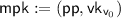and $\mathsf {msk}:=s$.

$\mathsf {KeyGen} (\mathsf {msk}= s,\mathsf {id}\in \{0,1\} ^n):$ :

Let $\mathsf {v}_0,\mathsf {v} _1,\dots ,\mathsf {v} _{n}$ be the root-to-leaf path for the identity $\mathsf {id}$, i.e. all the prefixes of $\mathsf {id}$. For $j = 0,\dots ,n-1$ compute $(\cdot , \sigma _{\mathsf {v} _j},\mathsf {x}_{\mathsf {v} _j}) :=\mathsf {NodeGen} (\mathsf {pp},\mathsf {v} _j,s)$. Further compute $(\cdot ,\sigma _{\mathsf {id}},\mathsf {lpk} _\mathsf {id},\mathsf {lsk} _\mathsf {id}) :=\mathsf {LeafGen} (\mathsf {pp},\mathsf {v} _{n},s)$. Output $\mathsf {sk}_\mathsf {id}:=( (\sigma _{\mathsf {v} _0},\mathsf {x}_{\mathsf {v} _0}),\dots ,(\sigma _{\mathsf {v} _n},\mathsf {x}_{\mathsf {v} _n}), \sigma _\mathsf {id},\mathsf {lpk} _\mathsf {id},\mathsf {lsk} _\mathsf {id})$.

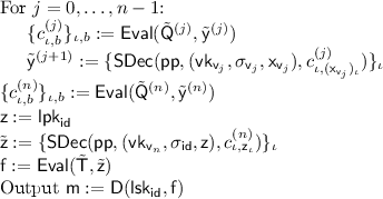
$\mathsf {Encrypt} (\mathsf {mpk}= (\mathsf {pp},\mathsf {vk}_{\mathsf {v}_0}),\mathsf {id}\in \{0,1\} ^n,\mathsf {m}):$ :

We will first describe two circuits that will be used by the encryption algorithm.

 

• $\mathsf {Q} [\mathsf {pp},\beta \in \{0,1\} , \mathsf {e}_Q = \{ (Y_{\iota ,0},Y_{\iota ,1}) \}_{\iota }](\mathsf {vk}):$ Compute and output

• $\mathsf {T} [\mathsf {m} ](\mathsf {lpk})$: Compute and output $\mathsf {E}(\mathsf {lpk},\mathsf {m})$.

  

 

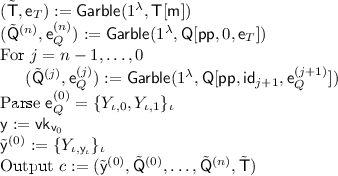
$\mathsf {Decrypt} (\mathsf {sk}_\mathsf {id}= ((\sigma _{\mathsf {v} _0},\mathsf {x}_{\mathsf {v} _0}),\dots ,(\sigma _{\mathsf {v} _n},\mathsf {x}_{\mathsf {v} _n}), \sigma _\mathsf {id},\mathsf {lpk} _\mathsf {id},\mathsf {lsk} _\mathsf {id}),{c}= (\tilde{\mathsf {y}}^{(0)},\tilde{\mathsf {Q}}^{(0)},\dots ,\tilde{\mathsf {Q}}^{(n)},\tilde{\mathsf {T}}))$ :

 

6.1 Correctness

We will first show that our scheme is correct. Note that by correctness of the garbling scheme $(\mathsf {Garble},\mathsf {Eval})$, we have that the evaluation of on the labels yields correctly formed ciphertexts of the OTSE scheme $(\mathsf {SSetup},\mathsf {SGen},\mathsf {SSign} \mathsf {SEnc},\mathsf {SDec})$. Next, by the correctness of $(\mathsf {SSetup},\mathsf {SGen},\mathsf {SSign},\mathsf {SEnc},\mathsf {SDec})$, we get that the decrypted values are correct labels for the next garbled circuit . Repeating this argument, we can argue that all output correct encryptions that are subsequently decrypted to correct input labels of the next garbled circuit in the sequence. Finally, the circuit outputs correct encryptions of the input labels of $\tilde{\mathsf {T}}$, which are again correctly decrypted to input labels for $\tilde{\mathsf {T}}$. Finally, the correctness of the garbling scheme $(\mathsf {Garble},\mathsf {Eval})$ guarantees that $\tilde{\mathsf {T}}$ outputs a correct encryption of the plaintext $\mathsf {m}$ under the leaf public key $\mathsf {lpk} _{\mathsf {id}}$, and the correctness of the public-key-encryption scheme $(\mathsf {KG},\mathsf {E},\mathsf {D})$ ensures that the decryption function $\mathsf {D}$ outputs the correct plaintext $\mathsf {m}$.

6.2 Proof of Security

We will now show that our scheme is fully secure.

Theorem 3

Assume that $(\mathsf {KG},\mathsf {E},\mathsf {D})$ is an $\mathsf {IND}^{\mathsf {CPA}}$-secure public key encryption scheme, $(\mathsf {SSetup},\mathsf {SGen},\mathsf {SSign},\mathsf {SEnc},\mathsf {SDec})$ is a $\mathsf {IND}^{\mathsf {OTSE}}$-secure OTSE scheme and that $(\mathsf {Garble},\mathsf {Eval})$ is a garbling scheme. Then the scheme $(\mathsf {Setup},\mathsf {KeyGen},\mathsf {Encrypt},\mathsf {Decrypt})$ is a fully secure IBE scheme.

We will split the proof of Theorem 3 into several lemmas. Let $\mathcal {A}$ be a PPT adversary with advantage $\epsilon$ against the fully secure $\mathsf {IND}^{\mathsf {IBE}}$-experiment and let in the following $\mathsf {v} _0,\dots ,\mathsf {v} _{n}$ always denote the root-to-leaf path for the challenge identity $\mathsf {id}^*$. Consider the following hybrids.

Hybrid $\mathcal {H} _0$ is identical to the real experiment $\mathsf {IND}^{\mathsf {IBE}} (\mathcal {A})$, except that we replace the pseudorandom function $F$ used for the generation of the identity keys by a lazily evaluated truly random function. In particular, each time we visit a new node during key generation we generate fresh keys for this node and store them. If these keys are needed later on, we retrieve them from a table of stored keys instead of generating new ones. By a standard argument it follows that the $\mathsf {IND}^{\mathsf {IBE}} (\mathcal {A})$-experiment and $\mathcal {H} _0$ are computationally indistinguishable, given that $F$ is a pseudorandom function.

In the remaining hybrids we will only change the way the challenge ciphertext ${c}^*$ is computed. First consider the computation of the challenge ciphertext ${c}^*$ in the extremal hybrids $\mathcal {H} _0$ and $\mathcal {H} _{2n + 3}$ (Fig. 7). While in $\mathcal {H} _0$ all garbled circuits are computed by the garbling algorithm $\mathsf {Garble}$, in $\mathcal {H} _{2n + 3}$ all garbled circuits are simulated. Moreover, in $\mathcal {H} _{2n + 3}$ the messages encrypted in the ciphertexts computed by the garbled circuits do not depend on the bit b, i.e. decryption of these ciphertexts always yields the same labels, regardless of which message-signature pair has been used to decrypt the encrypted labels. Notice that in $\mathcal {H} _{2n + 3}$ the garbled circuit $\tilde{\mathsf {T}}$ is simulated using $\mathsf {f} :=\mathsf {E}(\mathsf {lpk} _{\mathsf {id}^*},\mathsf {m} ^*)$, the encryption of the challenge message $\mathsf {m} ^*$ under the leaf public key $\mathsf {lpk} _{\mathsf {id}^*}$.

Fig. 7.

The extremal hybrids $\mathcal {H} _0$ and $\mathcal {H} _{2n + 3}$

We will show indistinguishability of $\mathcal {H} _0$ and $\mathcal {H} _{2n + 3}$ via the following hybrids. For $i = 0,\dots ,n-1$ define:

Hybrid $\mathcal {H} _{2i + 1}$. This hybrid is the same as $\mathcal {H} _{2i}$, except that we change the way $\tilde{\mathsf {Q}}^{(i)}$ and $\tilde{\mathsf {y}}^{(i)}$ are computed. Compute $\tilde{\mathsf {Q}}^{(i)}$ and $\tilde{\mathsf {y}}^{(i)}$ by $(\tilde{\mathsf {Q}}^{(i)},\tilde{\mathsf {y}}^{(i)}) :=\mathsf {GCSim} (\mathsf {Q},\mathsf {f}_Q ^{(i)})$.

Hybrid $\mathcal {H} _{2(i + 1)}$. This hybrid is identical to $\mathcal {H} _{2i + 1}$, except for the following change. Instead of computing we compute .

The final 3 hybrids are given as follows.

Hybrid $\mathcal {H} _{2n + 1}$. This hybrid is the same as $\mathcal {H} _{2n}$, except that we change the way $\tilde{\mathsf {Q}}^{(n)}$ and $\tilde{\mathsf {y}}^{(n)}$ are computed. Compute $\tilde{\mathsf {Q}}^{(n)}$ and $\tilde{\mathsf {y}}^{(n)}$ by , where .

Hybrid $\mathcal {H} _{2n + 2}$. This hybrid is the same as $\mathcal {H} _{2n + 1}$, except that we change how $\mathsf {f}_T$ is computed. Let $\mathsf {e}_T = \{Z_{\iota ,0},Z_{\iota ,1} \}_{\iota }$. Instead of computing $\mathsf {f}_T$ by $\mathsf {f}_T :=\{ (\mathsf {SEnc} (\mathsf {pp}, (\mathsf {vk}_{\mathsf {id}^*},\iota ,b), Z_{\iota ,b}) \}_{\iota , b}$ we compute $\mathsf {f}_T :=\{ (\mathsf {SEnc} (\mathsf {pp}, (\mathsf {vk}_{\mathsf {id}^*}, \iota , b), \tilde{\mathsf {z}}^{(n)}_\iota ) \}_{\iota , b}$.

Hybrid $\mathcal {H} _{2n + 3}$. This hybrid is the same as $\mathcal {H} _{2n + 2}$, except that we change the way $\tilde{\mathsf {T}}$ and $\tilde{\mathsf {z}}$ are computed. Compute $\tilde{\mathsf {T}}$ and $\tilde{\mathsf {z}}$ by $(\tilde{\mathsf {T}},\tilde{\mathsf {z}}) :=\mathsf {GCSim} (\mathsf {Q},\mathsf {f})$, where $\mathsf {f} :=\mathsf {E}(\mathsf {lpk} _\mathsf {id},\mathsf {m})$.

Lemma 1

We claim that for $i = 0,\dots ,n-1$ the hybrids $\mathcal {H} _{2i}$ and $\mathcal {H} _{2i+1}$ are computationally indistinguishable, given that $(\mathsf {Garble},\mathsf {Eval})$ is a secure garbling scheme.

Proof

Assume towards contradiction that $\mathcal {A}$ distinguishes between $\mathcal {H} _{2i}$ and $\mathcal {H} _{2i+1}$ with non-negligible advantage $\epsilon$. We will construct a distinguisher $\mathcal {R} ^\mathcal {A}$ that breaks the security of the garbling scheme with advantage $\epsilon$. $\mathcal {R}$ simulates the $\mathcal {H} _{2i}$ experiment faithfully with the adversary $\mathcal {A}$ until $\mathcal {A}$ requests a challenge ciphertext. Once $\mathcal {A}$ does request the challenge ciphertext, $\mathcal {R}$ computes

and sends the circuit $\mathsf {Q} [\mathsf {e}_Q ^{(i)}]$ and the input $\mathsf {y} ^{(i)}$ to the experiment. Once the experiment returns $\tilde{\mathsf {Q}}^{(i)},\tilde{\mathsf {y}}^{(i)}$, $\mathcal {R}$ computes

and returns ${c}^*$ to $\mathcal {A}$. $\mathcal {R}$ now continues the simulation of the $\mathcal {H} _{2i}$ experiment and outputs whatever the simulated $\mathcal {H} _{2i}$ experiment outputs.

Clearly, if $\mathcal {R}$ ’s challenge $\tilde{\mathsf {Q}}^{(i)},\tilde{\mathsf {y}}^{(i)}$ is distributed according to the real distribution, then the view of $\mathcal {A}$ in $\mathcal {R}$ ’s simulation is identical to the view of $\mathcal {A}$ in $\mathcal {H} _{2i}$. On the other hand, if $\mathcal {R}$ ’s challenge is distributed according to the simulated distribution, then the view of $\mathcal {A}$ in $\mathcal {R}$ ’s simulation is identical to the view of $\mathcal {A}$ in $\mathcal {H} _{2i+1}$. We conclude that

$$ \mathsf {Adv} (\mathcal {R} ^\mathcal {A}) = | \Pr [\mathcal {H} _{2i}(\mathcal {A}) = 1] - \Pr [\mathcal {H} _{2i+1}(\mathcal {A}) = 1] | \le \epsilon , $$

which contradicts the security of the garbling scheme $(\mathsf {Garble},\mathsf {Eval})$.

Lemma 2

We claim that for $i = 0,\dots ,n-1$ the hybrids $\mathcal {H} _{2i+1}$ and $\mathcal {H} _{2(i+1)}$ are computationally indistinguishable, given that $(\mathsf {SSetup},\mathsf {SGen},\mathsf {SSign},\mathsf {SEnc},\mathsf {SDec})$ is a selectively $\mathsf {IND}^{\mathsf {OTSE}}$-secure OTSE scheme.

Proof

Let q be the number of queries by $\mathcal {A}$ (including the challenge query), which gives us an upper bound for the number of distinct nodes visited at level i. We will construct an adversary $\mathcal {R} ^\mathcal {A}$ that breaks the $\mathsf {IND}^{\mathsf {OTSE}}$-security of $(\mathsf {SSetup},\mathsf {SGen},\mathsf {SSign},\mathsf {SEnc},\mathsf {SDec})$ in the multi-challenge setting with advantage $\epsilon /q$. $\mathcal {R}$ first guesses an index $k^*\in [q]$. $\mathcal {R}$ then generates keys

$$\begin{aligned} (\mathsf {vk}^*_0,\mathsf {sk}^*_0) :=\mathsf {SGen} (\mathsf {pp})\\ (\mathsf {vk}^*_1,\mathsf {sk}^*_1) :=\mathsf {SGen} (\mathsf {pp}) \end{aligned}$$

and sets $\mathsf {x}^*:=\mathsf {vk}_{\mathsf {v} _i \Vert 0} \Vert \mathsf {vk}_{\mathsf {v} _i \Vert 1}$ and sends the challenge message $\mathsf {x}^*$ to the $\mathsf {IND}^{\mathsf {OTSE}}$-experiment and receives a verification key $\mathsf {vk}$ and a signature $\sigma$ from the $\mathsf {IND}^{\mathsf {OTSE}}$-experiment.

$\mathcal {R}$ continues simulating the $\mathcal {H} _{2i + 1}$ experiment. Once the $k^*$-th distinct node $\mathsf {v} ^*$ on level i is visited, $\mathcal {R}$ modifies the $\mathsf {NodeGen}$ function for this node as follows.

When the corresponding signing keys are required for the $\mathsf {NodeGen}$ procedure on $\mathsf {v} ^*\Vert 0$ and $\mathsf {v} ^*\Vert 1$, use the corresponding signing keys $\mathsf {sk}_{\mathsf {v} ^*\Vert 0}$ and $\mathsf {sk}_{\mathsf {v} ^*\Vert 1}$ computed in the modified procedure above.

$\mathcal {R}$ now continues the simulation. Once $\mathcal {A}$ requests a challenge-ciphertext for an identity $\mathsf {id}^*$, $\mathcal {R}$ checks if $\mathsf {v} ^*$ is on the root-to-leaf path for $\mathsf {id}^*$ (i.e. if $\mathsf {v} ^*$ is a prefix of $\mathsf {id}^*$), and if not aborts and outputs a random bit. Otherwise, $\mathcal {R}$ generates the challenge ciphertext ${c}^*$ for $\mathcal {A}$ in the following way.

$\mathcal {R}$ now computes the messages $M^*_0 :=\{ Y_{\iota ,1 - \mathsf {x}^{(i+1)}_\iota }\}_{\iota }$ and $M^*_1 :=\{ Y_{\iota ,\mathsf {x}^{(i+1)}_\iota } \}_{\iota }$, sends the challenge messages $(M^*_0,M^*_1)$ to the $\mathsf {IND}^{\mathsf {OTSE}}$ experiment and receives a challenge ciphertext $C^*= (C^*_1,\dots ,C^*_\ell )$. Now $\mathcal {R}$ computes $\mathsf {f}_Q ^{(i+1)}$ by $\mathsf {f}_Q ^{(i+1)} :=\{ C_{\iota ,b} \}_{\iota }$, where $C_{\iota ,\mathsf {x}_\iota } :=\mathsf {SEnc} (\mathsf {pp}, (\mathsf {vk}_{\mathsf {v} _i},\mathsf {id}^*_{i+1} \cdot \ell + \iota ,\mathsf {x}^{(i+1)}_\iota ), Y_{\iota ,\mathsf {x}^{(i+1)}_\iota })$ and $C_{\iota ,1 - \mathsf {x}_\iota } :=C^*_\iota$. $\mathcal {R}$ continues the computation of the challenge ciphertext as follows.

and returns ${c}^*$ to $\mathcal {A}$. $\mathcal {R}$ now continues the simulation of the $\mathcal {H} _{2i+1}$ experiment and outputs whatever the simulated $\mathcal {H} _{2i+1}$ experiment outputs.

We will now compute the advantage of $\mathcal {R} ^\mathcal {A}$. First notice that the keys provided by $\mathcal {R}$ to $\mathcal {A}$ are distributed exactly as in $\mathcal {H} _{2i+1}$ (and therefore do not depend on $k^*$). If $\mathcal {R}$ guesses $k^*$ wrongly its advantage is 0. Let $\mathsf {E}$ be the event that $k^*$ has been guessed correctly. It clearly holds that $\Pr [\mathsf {E}] \ge 1/q$. Assume now that the event $\mathsf {E}$ holds. If the challenge bit $b^*$ of the $\mathsf {IND}^{\mathsf {OTSE}}$ experiment is 0, then the view of $\mathcal {A}$ in $\mathcal {R}$ ’s simulation is distributed exactly as in experiment $\mathcal {H} _{2i+1}$. On the other hand, if $b^*= 1$ then the view of $\mathcal {A}$ is distributed exactly as in experiment $\mathcal {H} _{2(i+1)}$. Thus we can conclude

$$\begin{aligned} \mathsf {Adv} (\mathcal {R} ^\mathcal {A})&= \Pr [\mathsf {E}] \cdot | \Pr [\mathcal {H} _{2i+1}(\mathcal {A}) = 1] - \Pr [\mathcal {H} _{2(i+1)}(\mathcal {A}) = 1]|\\&\ge \Pr [\mathsf {E}] \cdot \epsilon \\&\ge \epsilon / q. \end{aligned}$$

Lemma 3

We claim that the hybrids $\mathcal {H} _{2n}$ and $\mathcal {H} _{2n+1}$ are computationally indistinguishable, given that $(\mathsf {Garble},\mathsf {Eval})$ is a secure garbling scheme.

The proof proceeds analogous to the proof of Lemma 1.

Lemma 4

We claim that the hybrids $\mathcal {H} _{2n+1}$ and $\mathcal {H} _{2n+2}$ are computationally indistinguishable, given that the OTSE-scheme $(\mathsf {SSetup},\mathsf {SGen},\mathsf {SSign},\mathsf {SEnc},\mathsf {SDec})$ is $\mathsf {IND}^{\mathsf {OTSE}}$-secure.

The proof follows analogous to the proof of Lemma 2.

Lemma 5

We claim that the hybrids $\mathcal {H} _{2n + 2}$ and $\mathcal {H} _{2n+3}$ are computationally indistinguishable, given that $(\mathsf {Garble},\mathsf {Eval},\mathsf {GCSim})$ is a secure garbling scheme.

Again, the proof follows analogous to the proof of Lemma 1.

Lemma 6

The advantage of $\mathcal {A}$ in $\mathcal {H} _{2 n + 3}$ is negligible, given that $(\mathsf {KG},\mathsf {E},\mathsf {D})$ is $\mathsf {IND}^{\mathsf {CPA}}$-secure.

Proof

We will construct an adversary $\mathcal {R} ^\mathcal {A}$ that breaks the $\mathsf {IND}^{\mathsf {CPA}}$ security of $(\mathsf {KG},\mathsf {E},\mathsf {D})$ with advantage $\epsilon$. $\mathcal {R}$ simulates $\mathcal {H} _{2 n + 3}$ faithfully, with the exception that it uses its own challenge public key $\mathsf {pk}^*$ as public key for the leaf $\mathsf {id}^*$, i.e. it sets $\mathsf {lpk} _{\mathsf {id}^*} :=\mathsf {pk}^*$. It forwards $\mathcal {A}$ ’s challenge messages $\mathsf {m} _0$ and $\mathsf {m} _1$ to the $\mathsf {IND}^{\mathsf {CPA}}$ experiment and uses its own challenge ciphertext $c^*$ as the ciphertext $\mathsf {f}$ in the computation of the challenge ciphertext ${c}^*$. It follows that $\mathcal {R}$ simulates $\mathcal {H} _{4n + 3}$ perfectly and therefore $\mathsf {Adv} _{\mathsf {IND}^{\mathsf {CPA}}}(\mathcal {R} ^\mathcal {A}) = \mathsf {Adv} _{\mathcal {H} _{4n + 3}}(\mathcal {A})$.

This concludes the proof of Theorem 3.

7 Achieving Selectively Secure HIBE

We will now add a delegation mechanism to the IBE scheme constructed in the last Section, yielding the construction of a hierarchical IBE scheme. The basic idea is as follows. Instead of putting the public keys of the $\mathsf {IND}^{\mathsf {CPA}}$-secure scheme only into the leaf nodes of the tree, we will put such public keys into every node of the tree. This means that every node of the (unbounded size) tree can effectively be used in the same way we used the leaf nodes in the scheme of the last Section.

Since we want to be able to delegate the ability to delegate HIBE keys for entire sub-trees, we need to work with a pseudorandom function supporting this kind of delegation. We therefore use the delegatable pseudorandom functions defined in Sect. 2.6 for this task.

In our scheme, the delegated master secret key for an identity $\mathsf {id}$ consist of the identity secret key for $\mathsf {id}$ and a delegated PRF seed $s_{\mathsf {id}}$. This enables the delegator to compute identity secret keys for all the nodes in the sub-tree of $\mathsf {id}$.

Let $(\mathsf {SSetup},\mathsf {SGen},\mathsf {SSign},\mathsf {SEnc},\mathsf {SDec})$ be an $\mathsf {IND}^{\mathsf {OTSE}}$-secure OTSE scheme, $(F,F.\mathsf {Delegate})$ be a delegatable pseudorandom function and $(\mathsf {KG},\mathsf {E},\mathsf {D})$ be a standard public key encryption scheme. We assume for convenience that the pseudorandom function $F$ has two output registers, $F_1$ and $F_2$. Assume that both the verification keys of $(\mathsf {SSetup},\mathsf {SGen},\mathsf {SSign},\mathsf {SEnc},\mathsf {SDec})$ and the public keys of $(\mathsf {KG},\mathsf {E},\mathsf {D})$ have length $\ell$ and let $d = 3 \ell$.

Again, we will first define a function $\mathsf {NodeGen}$ that provides access to the keys stored in the tree. As mentioned above, we do not make distinctions between leaf nodes and non-leaf nodes anymore but store a local public key $\mathsf {lpk} _\mathsf {v}$ at every node $\mathsf {v}$. $\mathsf {NodeGen}$ takes as input a node identifier $\mathsf {v}$ and a pseudorandom function seed s and outputs a verification key , signatures $\sigma _{\mathsf {v}}$, auxiliary information $\mathsf {x}_\mathsf {v}$ and a secret key $\mathsf {lsk} _\mathsf {v}$. Again, we use the convention that the variable $\iota$ runs over $[\ell ]$ and b over $\{0,1\}$.

The HIBE scheme $(\mathsf {Setup},\mathsf {Delegate},\mathsf {KeyGen},\mathsf {Encrypt},\mathsf {Decrypt})$ is given by the following algorithms.

 

$\mathsf {Setup} (1^{\lambda }):$ :

Let $\mathsf {v}_0$ be the root-node. Choose a random seed s for the pseudorandom function $F$. Compute $\mathsf {pp}:=\mathsf {SSetup} (1^\lambda ,3 \cdot \ell )$ and $(\mathsf {vk}_{\mathsf {v}_0},\cdot ,\cdot ,\cdot ) :=\mathsf {NodeGen} (\mathsf {pp},\mathsf {v}_0,s)$. Output $\mathsf {mpk}:=\mathsf {vk}_{\mathsf {v}_0}$ and $\mathsf {msk}:=s$.

$\mathsf {Delegate} (\mathsf {msk}= s,\mathsf {id}\in \{0,1\} ^*)$::

Set $n :=|\mathsf {id}|$. Let $\mathsf {v}_0,\mathsf {v} _1,\dots ,\mathsf {v} _{n}$ be the root-to-leaf path for the identity $\mathsf {id}$, i.e. all the prefixes of $\mathsf {id}$. For $j = 0,\dots ,n-1$ compute $(\cdot , \sigma _{\mathsf {v} _j},\mathsf {x}_\mathsf {v},\cdot ) :=\mathsf {NodeGen} (\mathsf {pp},\mathsf {v} _j,s)$. Compute $s_\mathsf {id}:=F.\mathsf {Delegate} (s,\mathsf {id})$. Output $( (\sigma _{\mathsf {v} _0},\mathsf {x}_{\mathsf {v} _0}),\dots ,(\sigma _{\mathsf {v} _n},\mathsf {x}_{\mathsf {v} _n}),s_\mathsf {id})$ ⁷

$\mathsf {KeyGen} (\mathsf {msk}^{\mathsf {HIBE}}_{\mathsf {id}'} = ((\sigma _{\mathsf {v} _0},\mathsf {x}_{\mathsf {v} _0}),\dots ,(\sigma _{\mathsf {v} _{|\mathsf {id}'|}},\mathsf {x}_{\mathsf {v} _{|\mathsf {id}'|}}),s_{\mathsf {id}'}),\mathsf {id}\in \{0,1\} ^*):$ :

Set $n :=|\mathsf {id}|$. Let $\mathsf {v} _{ |\mathsf {id}'|},\dots ,\mathsf {v} _{|\mathsf {id}'| + |\mathsf {id}|}$ be the path from $\mathsf {id}'$ to $\mathsf {id}' \Vert \mathsf {id}$, i.e. $\mathsf {id}'$ concatenated with all the prefixes of $\mathsf {id}$. For $j = |\mathsf {id}'|,\dots ,|\mathsf {id}'| + |\mathsf {id}| -1$ compute $(\cdot , \sigma _{\mathsf {v} _j},\mathsf {x}_\mathsf {v},\mathsf {lsk} _\mathsf {v}) :=\mathsf {NodeGen} (\mathsf {pp},\mathsf {v} _j,s_{\mathsf {id}'})$. Output $\mathsf {sk}_\mathsf {id}:=((\sigma _{\mathsf {v} _0},\mathsf {x}_{\mathsf {v} _0}),\dots ,(\sigma _{\mathsf {v} _{|\mathsf {id}'| + |\mathsf {id}|}},\mathsf {x}_{\mathsf {v} _{|\mathsf {id}'| + |\mathsf {id}|}}), \sigma _\mathsf {id},\mathsf {lsk} _\mathsf {id})$

$\mathsf {Encrypt} (\mathsf {mpk}= \mathsf {vk}_{\mathsf {v}_0},\mathsf {id}\in \{0,1\} ^*,\mathsf {m}):$ :

We will first describe two circuits that will be used by the encryption algorithm. The mode $\beta = 2$ of the circuit $\mathsf {Q}$ targets a local public key.

 

• $\mathsf {Q} [\mathsf {pp},\beta \in \{0,1,2\}, \mathsf {e}_Q = \{ (Y_{\iota ,0},Y_{\iota ,1}) \}_{\iota }](\mathsf {vk}):$ Compute and then output $\{ \mathsf {SEnc} (\mathsf {pp},(\mathsf {vk},\beta \cdot \ell + \iota ,b), Y_{\iota ,b}) \}_{\iota , b}$

• $\mathsf {T} [\mathsf {m} ](\mathsf {lpk})$: Compute and output $\mathsf {E}(\mathsf {lpk},\mathsf {m})$.

  

 

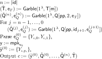
$\mathsf {Decrypt} (\mathsf {sk}_\mathsf {id}= ( (\sigma _{\mathsf {v} _0},\mathsf {x}_{\mathsf {v} _0}),\dots , (\sigma _{\mathsf {v} _n},\mathsf {x}_{\mathsf {v} _n}), \sigma _\mathsf {id},\mathsf {lpk} _\mathsf {id},\mathsf {lsk} _\mathsf {id}),{c}= (\tilde{\mathsf {y}}^{(0)},\tilde{\mathsf {Q}}^{(0)},\dots ,\tilde{\mathsf {Q}}^{(n)},\tilde{\mathsf {T}}))$ :

 

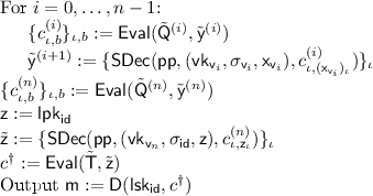
7.1 Correctness

Correctness of the scheme follows by the same argument as for the scheme in Sect. 6. Moreover, correctness of the delegation mechanism follows directly from the the correctness of the delegation mechanism $F.\mathsf {Delegate}$.

7.2 Proof of Security

We will now show that our scheme is $\mathsf {sel\text {-}IND}^{\mathsf {HIBE}}$-secure.

Theorem 4

Assume that $(\mathsf {KG},\mathsf {E},\mathsf {D})$ is an $\mathsf {IND}^{\mathsf {CPA}}$-secure public-key-encryption scheme, $(\mathsf {SSetup},\mathsf {SGen},\mathsf {SSign},\mathsf {SEnc},\mathsf {SDec})$ is an $\mathsf {IND}^{\mathsf {OTSE}}$-secure one-time signature with encryption scheme and that $(\mathsf {Garble},\mathsf {Eval})$ is a garbling scheme. Then $(\mathsf {Setup},\mathsf {Delegate},\mathsf {KeyGen},\mathsf {Encrypt},\mathsf {Decrypt})$ is a $\mathsf {sel\text {-}IND}^{\mathsf {HIBE}}$-secure HIBE scheme.

We will split the proof of Theorem 4 into several lemmas. Let $\mathcal {A}$ be a PPT adversary with advantage $\epsilon$ against the $\mathsf {sel\text {-}IND}^{\mathsf {HIBE}}$-experiment, let $\mathsf {id}^*$ be the challenge identity, which is selectively chosen by $\mathcal {A}$ at the beginning of the experiment and let $n^*:=|\mathsf {id}^*|$ be the length of the challenge identity. Let in the following $\mathsf {v} _0,\dots ,\mathsf {v} _{n^*}$ always denote the root-to-leaf path for the challenge identity $\mathsf {id}^*$.

We will start by providing an overview of the hybrids.

Hybrid $\mathcal {H} _0$. This hybrid is identical to the real experiment $\mathsf {sel\text {-}IND}^{\mathsf {HIBE}} _\mathcal {A}$, except that on the challenge-path $\mathsf {v} _0,\dots ,\mathsf {v} _{n}$ we replace the pseudorandom function $F$ used for the generation of the identity keys by a function H, which is truly random on the path from the root to the challenge identity and identical to $F(s,\cdot )$ everywhere else. This means, in particular, that we can choose the all the keys on the path from the root to the challenge identity in advance and with truly random coins. It follows directly from the pseudorandomness property of the delegatable pseudorandom function $(F,F.\mathsf {Delegate})$ that the experiments $\mathsf {IND}^{\mathsf {IBE}} (\mathcal {A})$ and $\mathcal {H} _0$ are computationally indistinguishable.

In the remaining hybrids, we will only change the way the challenge ciphertext ${c}^*$ is computed. For $i = 0,\dots ,n^*-1$ we define the hybrids $\mathcal {H} _0,\dots ,\mathcal {H} _{2 n^*+ 3}$. As in the last Section, we will first provide an overview of the extremal hybrids $\mathcal {H} _0$ and $\mathcal {H} _{2n^*+ 3}$ in Fig. 8.

Fig. 8.

The extremal hybrids $\mathcal {H} _0$ and $\mathcal {H} _{2n^*+ 3}$

For $i = 0,\dots ,n^*- 1$ define the following hybrids.

Hybrid $\mathcal {H} _{2i + 1}$. This hybrid is the same as $\mathcal {H} _{2i}$, except that we change the way $\tilde{\mathsf {Q}}^{(i)}$ and $\tilde{\mathsf {y}}^{(i)}$ are computed. Compute $\tilde{\mathsf {Q}}^{(i)}$ and $\tilde{\mathsf {y}}^{(i)}$ by $(\tilde{\mathsf {Q}}^{(i)},\tilde{\mathsf {y}}^{(i)}) :=\mathsf {GCSim} (\mathsf {Q},\mathsf {f}_Q ^{(i)})$.

Hybrid $\mathcal {H} _{2(i + 1)}$. This hybrid is identical to $\mathcal {H} _{2i + 1}$, except for the following change. Instead of computing $\mathsf {f}_Q ^{(i+1)} :=\{ \mathsf {SEnc} ( \mathsf {pp}, (\mathsf {vk}_{\mathsf {v} _i},\mathsf {id}^*_{i+1} \cdot \ell + \iota , b),Y_{\iota ,b}) \}_{\iota , b}$ we compute $\mathsf {f}_Q ^{(i+1)} :=\{ \mathsf {SEnc} (\mathsf {pp}, (\mathsf {vk}_{\mathsf {v} _i},\mathsf {id}^*_{i+1} \cdot \ell + \iota , b), \tilde{\mathsf {y}}^{(i+1)}_\iota ) \}_{\iota , b}$

The final 3 hybrids are given as follows.

Hybrid $\mathcal {H} _{2n^*+ 1}$. This hybrid is the same as $\mathcal {H} _{2n^*}$, except that we change the way $\tilde{\mathsf {Q}}^{(n^*)}$ and $\tilde{\mathsf {y}}^{(n^*)}$ are computed. Compute $\tilde{\mathsf {Q}}^{(n^*)}$ and $\tilde{\mathsf {y}}^{(n^*)}$ by $(\tilde{\mathsf {Q}}^{(n^*)},\tilde{\mathsf {y}}^{(n^*)}) :=\mathsf {GCSim} (\mathsf {Q},\mathsf {f}_T)$.

Hybrid $\mathcal {H} _{2n^*+ 2}$. This hybrid is the same as $\mathcal {H} _{2n^*+ 1}$, except that we change how $\mathsf {f}_T$ is computed. Let $\mathsf {e}_T = \{ Z_{\iota ,0},Z_{\iota ,1} \}_{\iota }$. Instead of computing $\mathsf {f}_T$ by $\mathsf {f}_T :=\{ (\mathsf {SEnc} (\mathsf {pp}, (\mathsf {vk}\mathsf {vk}_{\mathsf {v} _{n^*}},\iota , b), Z_{\iota ,b}) \}_{\iota , b}$ we compute $\mathsf {f}_T :=\{ (\mathsf {SEnc} (\mathsf {pp}, (\mathsf {vk}_{n^*},\iota , b), \tilde{\mathsf {z}}^{(n^*)}_\iota ) \}_{\iota , b}$.

Hybrid $\mathcal {H} _{2n^*+ 3}$. This hybrid is the same as $\mathcal {H} _{2n^*+ 2}$, except that we change the way $\tilde{\mathsf {T}}$ and $\tilde{\mathsf {z}}$ are computed. Compute $\tilde{\mathsf {T}}$ and $\tilde{\mathsf {z}}$ by $(\tilde{\mathsf {T}},\tilde{\mathsf {z}}) :=\mathsf {GCSim} (\mathsf {Q},\mathsf {f})$, where $\mathsf {f} :=\mathsf {E}(\mathsf {lpk} _{\mathsf {id}^*},\mathsf {m} ^*)$.

Lemma 7

We claim that for $i = 0,\dots ,n^*-1$ the hybrids $\mathcal {H} _{2i}$ and $\mathcal {H} _{2i+1}$ are computationally indistinguishable, given that $(\mathsf {Garble},\mathsf {Eval})$ is a secure garbling scheme.

Proof

Assume towards contradiction that $\mathcal {A}$ distinguishes between $\mathcal {H} _{2i}$ and $\mathcal {H} _{2i+1}$ with non-negligible advantage $\epsilon$. We will construct a distinguisher $\mathcal {R} ^\mathcal {A}$ that breaks the security of the garbling scheme with advantage $\epsilon$. $\mathcal {R}$ simulates the $\mathcal {H} _{2i}$ experiment faithfully with the adversary $\mathcal {A}$ until $\mathcal {A}$ requests a challenge ciphertext. Once $\mathcal {A}$ does request the challenge ciphertext, $\mathcal {R}$ computes

and sends the circuit $\mathsf {Q} [\mathsf {e}_Q ^{(i)}]$ and the input $\mathsf {y} ^{(i)}$ to the experiment. Once the experiment returns $\tilde{\mathsf {Q}}^{(i)},\tilde{\mathsf {y}}^{(i)}$, $\mathcal {R}$ computes

and returns ${c}^*$ to $\mathcal {A}$. $\mathcal {R}$ now continues the simulation of the $\mathcal {H} _{2i}$ experiment and outputs whatever the simulated $\mathcal {H} _{2i}$ experiment outputs.

Clearly, if $\mathcal {R}$ ’s challenge $\tilde{\mathsf {Q}}^{(i)},\tilde{\mathsf {y}}^{(i)}$ is distributed according to the real distribution, then the view of $\mathcal {A}$ in $\mathcal {R}$ ’s simulation is identical to the view of $\mathcal {A}$ in $\mathcal {H} _{2i}$. On the other hand, if $\mathcal {R}$ ’s challenge is distributed according to the simulated distribution, then the view of $\mathcal {A}$ in $\mathcal {R}$ ’s simulation is identical to the view of $\mathcal {A}$ in $\mathcal {H} _{2i+1}$. We conclude that

$$ \mathsf {Adv} (\mathcal {R} ^\mathcal {A}) = | \Pr [\mathcal {H} _{2i}(\mathcal {A}) = 1] - \Pr [\mathcal {H} _{2i+1}(\mathcal {A}) = 1] | \le \epsilon , $$

which contradicts the security of the garbling scheme $(\mathsf {Garble},\mathsf {Eval})$.

Lemma 8

We claim that for $i = 0,\dots ,n^*-1$ the hybrids $\mathcal {H} _{2i+1}$ and $\mathcal {H} _{2(i+1)}$ are computationally indistinguishable, given that $(\mathsf {SSetup},\mathsf {SGen},\mathsf {SSign},\mathsf {SEnc},\mathsf {SDec})$ is an $\mathsf {IND}^{\mathsf {OTSE}}$-secure IBE scheme.

Proof

We will construct an adversary $\mathcal {R} ^\mathcal {A}$ that breaks the multi-challenge $\mathsf {IND}^{\mathsf {OTSE}}$-security of $(\mathsf {SSetup},\mathsf {SGen},\mathsf {SSign},\mathsf {SEnc},\mathsf {SDec})$ with advantage $\epsilon$. Let $\mathsf {v} ^*= \mathsf {v} _i$ be the i-th node on the challenge-path. Let $\mathsf {pp}$ be the public parameters passed to $\mathcal {R}$. $\mathcal {R}$ first generates keys for the children $\mathsf {v} ^*\Vert 0$ and $\mathsf {v} ^*\Vert 1$ of $\mathsf {v} ^*$ by

$$ (\mathsf {vk}^*_b,\mathsf {sk}^*_b) :=\mathsf {SGen} (\mathsf {pp}) $$

if $\mathsf {v} ^*\Vert b$ is on the challenge path and

$$ (\mathsf {vk}^*_b,\mathsf {sk}^*_b) :=\mathsf {SGen} (\mathsf {pp};F(s,\mathsf {v} ^*\Vert b)) $$

otherwise. Next, $\mathcal {R}$ generates the local key $\mathsf {lpk} _{\mathsf {v} ^*}$ by $(\mathsf {lpk} ^*,\mathsf {lsk} ^*) :=\mathsf {KeyGen} (1^\lambda )$. Now $\mathcal {R}$ sets $\mathsf {x}^*:=\mathsf {vk}_{\mathsf {v} ^*\Vert 0} \Vert \mathsf {vk}_{\mathsf {v} ^*\Vert 1} \Vert \mathsf {lpk} _{\mathsf {v} ^*}$, sends the challenge message $\mathsf {x}^*$ to the $\mathsf {IND}^{\mathsf {OTSE}}$-experiment and receives a verification key $\mathsf {vk}$ and a signature $\sigma$.

$\mathcal {R}$ now chooses the keys for all nodes on the root-to-leaf path as in $\mathcal {H} _{2i + 1}$, except for the keys of $\mathsf {v} ^*$, which are chosen as follows.

When the corresponding secret keys are required for the $\mathsf {NodeGen}$ procedure on $\mathsf {v} ^*\Vert 0$ and $\mathsf {v} ^*\Vert 1$, use the corresponding secret keys $\mathsf {sk}_{\mathsf {v} ^*\Vert 0}$ and $\mathsf {sk}_{\mathsf {v} ^*\Vert 1}$ set above in the modified procedure above.

$\mathcal {R}$ now continues the simulation. Once $\mathcal {A}$ requests a challenge-ciphertext for the identity $\mathsf {id}^*$, $\mathcal {R}$ generates the challenge ciphertext ${c}^*$ for $\mathcal {A}$ in the following way.

$\mathcal {R}$ now computes the messages $M^*_0 :=\{ Y_{\iota ,1 - \mathsf {x}^{(i+1)}_\iota }\}_{\iota }$ and $M^*_1 :=\{ Y_{\iota ,\mathsf {x}^{(i+1)}_\iota } \}_{\iota }$, sends the challenge messages $(M^*_0,M^*_1)$ to the $\mathsf {IND}^{\mathsf {OTSE}}$-experiment and receives a challenge ciphertext $C^*= (C^*_1,\dots ,C^*_\ell )$. Now $\mathcal {R}$ computes $\mathsf {f}_Q ^{(i+1)}$ by $\mathsf {f}_Q ^{(i+1)} :=\{ C_{\iota ,b} \}_{\iota \in [\ell ]}$, where $C_{\iota ,\mathsf {x}_\iota } :=\mathsf {SEnc} (\mathsf {pp}, (\mathsf {vk}_{\mathsf {v} ^*}, \beta \cdot \ell +\iota ,\mathsf {x}^{(i+1)}_\iota ), Y_{\iota ,\mathsf {x}^{(i+1)}_\iota })$ and $C_{\iota ,1 - \mathsf {x}_\iota } :=C^*_\iota$.

and returns ${c}^*$ to $\mathcal {A}$. $\mathcal {R}$ now continues the simulation of the $\mathcal {H} _{2i+1}$ experiment and outputs whatever the simulated $\mathcal {H} _{2i+1}$ experiment outputs.

We will now compute the advantage of $\mathcal {R} ^\mathcal {A}$. First notice that the keys provided by $\mathcal {R}$ to $\mathcal {A}$ are distributed exactly as in $\mathcal {H} _{2i+1}$ (and therefore do not depend on $i^*$). If the challenge bit $b^*$ of the $\mathsf {IND}^{\mathsf {OTSE}}$-experiment is 0, then the view of $\mathcal {A}$ in $\mathcal {R}$ ’s simulation is distributed exactly as in experiment $\mathcal {H} _{2i+1}$. On the other hand, if $b^*= 1$ then the view of $\mathcal {A}$ is distributed exactly as in experiment $\mathcal {H} _{2(i+1)}$. Thus we can conclude

$$\begin{aligned} \mathsf {Adv} (\mathcal {R} ^\mathcal {A})&= | \Pr [\mathcal {H} _{2i+1}(\mathcal {A}) = 1] - \Pr [\mathcal {H} _{2(i+1)}(\mathcal {A}) = 1]| \ge \epsilon \end{aligned}$$

Lemma 9

We claim that the hybrids $\mathcal {H} _{2n}$ and $\mathcal {H} _{2n+1}$ are computationally indistinguishable, given that $(\mathsf {Garble},\mathsf {Eval})$ is a secure garbling scheme.

The proof proceeds analogous to the proof of Lemma 7.

Lemma 10

We claim that the hybrids $\mathcal {H} _{2n+1}$ and $\mathcal {H} _{2n+2}$ are computationally indistinguishable, given that the OTSE scheme $(\mathsf {SSetup},\mathsf {SGen},\mathsf {SSign},\mathsf {SEnc},\mathsf {SDec})$ is $\mathsf {IND}^{\mathsf {OTSE}}$-secure.

The proof follows analogous to the proof of Lemma 8.

Lemma 11

We claim that the hybrids $\mathcal {H} _{2n + 2}$ and $\mathcal {H} _{2n+3}$ are computationally indistinguishable, given that $(\mathsf {Garble},\mathsf {Eval})$ is a secure garbling scheme.

Again, the proof follows analogous to the proof of Lemma 7.

Lemma 12

The advantage of $\mathcal {A}$ in $\mathcal {H} _{2 n + 3}$ is negligible, given that $(\mathsf {KG},\mathsf {E},\mathsf {D})$ is $\mathsf {IND}^{\mathsf {CPA}}$-secure.

Proof

We will construct an adversary $\mathcal {R} ^\mathcal {A}$ that breaks the $\mathsf {IND}^{\mathsf {CPA}}$-security of $(\mathsf {KG},\mathsf {E},\mathsf {D})$ with advantage $\epsilon$. $\mathcal {R}$ simulates $\mathcal {H} _{2 n^*+ 3}$ faithfully, with the exception that it uses its own challenge public key $\mathsf {pk}^*$ as public key $\mathsf {lpk} _{\mathsf {id}^*}$ for the identity $\mathsf {id}^*$, i.e. it sets $\mathsf {lpk} _{\mathsf {id}^*} :=\mathsf {pk}^*$. It forwards $\mathcal {A}$ ’s challenge messages $\mathsf {m} _0$ and $\mathsf {m} _1$ to the $\mathsf {IND}^{\mathsf {CPA}}$-experiment and uses its own challenge ciphertext $c^*$ as the ciphertext $\mathsf {f}$ in the computation of the challenge ciphertext ${c}^*$. It follow directly that $\mathcal {R}$ simulates $\mathcal {H} _{4n^*+ 3}$ perfectly and therefore $\mathsf {Adv} _{\mathsf {IND}^{\mathsf {CPA}}}(\mathcal {R} ^\mathcal {A}) = \mathsf {Adv} _{\mathcal {H} _{4n^*+ 3}}(\mathcal {A})$.

This concludes the proof of Theorem 4.

References

Agrawal, S., Boyen, X.: Identity-based encryption from lattices in the standard model (2009)
Agrawal, S., Boneh, D., Boyen, X.: Efficient lattice (H)IBE in the standard model. In: Gilbert, H. (ed.) EUROCRYPT 2010. LNCS, vol. 6110, pp. 553–572. Springer, Heidelberg (2010). https://doi.org/10.1007/978-3-642-13190-5_28
Agrawal, S., Boneh, D., Boyen, X.: Lattice basis delegation in fixed dimension and shorter-ciphertext hierarchical IBE. In: Rabin, T. (ed.) CRYPTO 2010. LNCS, vol. 6223, pp. 98–115. Springer, Heidelberg (2010). https://doi.org/10.1007/978-3-642-14623-7_6
Abdalla, M., Catalano, D., Dent, A.W., Malone-Lee, J., Neven, G., Smart, N.P.: Identity-based encryption gone wild. In: Bugliesi, M., Preneel, B., Sassone, V., Wegener, I. (eds.) ICALP 2006. LNCS, vol. 4052, pp. 300–311. Springer, Heidelberg (2006). https://doi.org/10.1007/11787006_26
Abdalla, M., Fiore, D., Lyubashevsky, V.: From selective to full security: semi-generic transformations in the standard model. In: Fischlin, M., Buchmann, J., Manulis, M. (eds.) PKC 2012. LNCS, vol. 7293, pp. 316–333. Springer, Heidelberg (2012). https://doi.org/10.1007/978-3-642-30057-8_19
Asharov, G., Segev, G.: Limits on the power of indistinguishability obfuscation and functional encryption. In: Guruswami, V. (ed.) 56th Annual Symposium on Foundations of Computer Science, Berkeley, CA, USA, 17–20 October 2015, pp. 191–209. IEEE Computer Society Press (2015)
Boneh, D., Boyen, X.: Efficient selective-ID secure identity-based encryption without random oracles. In: Cachin, C., Camenisch, J.L. (eds.) EUROCRYPT 2004. LNCS, vol. 3027, pp. 223–238. Springer, Heidelberg (2004). https://doi.org/10.1007/978-3-540-24676-3_14
Boneh, D., Boyen, X.: Secure identity based encryption without random oracles. In: Franklin, M. (ed.) CRYPTO 2004. LNCS, vol. 3152, pp. 443–459. Springer, Heidelberg (2004). https://doi.org/10.1007/978-3-540-28628-8_27
Boneh, D., Boyen, X., Goh, E.-J.: Hierarchical identity based encryption with constant size ciphertext. In: Cramer, R. (ed.) EUROCRYPT 2005. LNCS, vol. 3494, pp. 440–456. Springer, Heidelberg (2005). https://doi.org/10.1007/11426639_26
Boneh, D., Franklin, M.: Identity-based encryption from the weil pairing. In: Kilian, J. (ed.) CRYPTO 2001. LNCS, vol. 2139, pp. 213–229. Springer, Heidelberg (2001). https://doi.org/10.1007/3-540-44647-8_13
Bellare, M., Hoang, V.T., Rogaway, P.: Foundations of garbled circuits. In: Yu, T., Danezis, G., Gligor, V.D. (eds.) 19th Conference on Computer and Communications Security, ACM CCS 2012, Raleigh, NC, USA, 16–18 October 2012, pp. 784–796. ACM Press (2012)
Bellare, M., Rogaway, P.: Random oracles are practical: a paradigm for designing efficient protocols. In: Ashby, V. (ed.) 1st Conference on Computer and Communications Security, ACM CCS 1993, Fairfax, Virginia, USA, 3–5 November 1993, pp. 62–73. ACM Press (1993)
Cho, C., Döttling, N., Garg, S., Gupta, D., Miao, P., Polychroniadou, A.: Laconic oblivious transfer and its applications. In: Katz, J., Shacham, H. (eds.) CRYPTO 2017. LNCS, vol. 10402, pp. 33–65. Springer, Cham (2017). https://doi.org/10.1007/978-3-319-63715-0_2
Canetti, R., Halevi, S., Katz, J.: Chosen-ciphertext security from identity-based encryption. In: Cachin, C., Camenisch, J.L. (eds.) EUROCRYPT 2004. LNCS, vol. 3027, pp. 207–222. Springer, Heidelberg (2004). https://doi.org/10.1007/978-3-540-24676-3_13
Cash, D., Hofheinz, D., Kiltz, E., Peikert, C.: Bonsai trees, or how to delegate a lattice basis. In: Gilbert, H. (ed.) EUROCRYPT 2010. LNCS, vol. 6110, pp. 523–552. Springer, Heidelberg (2010). https://doi.org/10.1007/978-3-642-13190-5_27
Cocks, C.: An identity based encryption scheme based on quadratic residues. In: Honary, B. (ed.) Cryptography and Coding 2001. LNCS, vol. 2260, pp. 360–363. Springer, Heidelberg (2001). https://doi.org/10.1007/3-540-45325-3_32
Döttling, N., Garg, S.: Identity-based encryption from the diffie-hellman assumption. In: Katz, J., Shacham, H. (eds.) CRYPTO 2017. LNCS, vol. 10401, pp. 537–569. Springer, Cham (2017). https://doi.org/10.1007/978-3-319-63688-7_18
Diffie, W., Hellman, M.E.: New directions in cryptography. IEEE Trans. Inf. Theory 22(6), 644–654 (1976)
Goldreich, O., Goldwasser, S., Micali, S.: How to construct random functions (extended abstract). In: 25th Annual Symposium on Foundations of Computer Science, Singer Island, Florida, 24–26 October 1984, pp. 464–479. IEEE Computer Society Press (1984)
Goldreich, O., Goldwasser, S., Micali, S.: How to construct random functions. J. ACM 33(4), 792–807 (1986)
Gentry, C., Halevi, S.: Hierarchical identity based encryption with polynomially many levels. In: Reingold, O. (ed.) TCC 2009. LNCS, vol. 5444, pp. 437–456. Springer, Heidelberg (2009). https://doi.org/10.1007/978-3-642-00457-5_26
Gaborit, P., Hauteville, A., Phan, D.H., Tillich, J.-P.: Identity-based encryption from codes with rank metric. In: Katz, J., Shacham, H. (eds.) CRYPTO 2017. LNCS, vol. 10403, pp. 194–224. Springer, Cham (2017). https://doi.org/10.1007/978-3-319-63697-9_7
Gentry, C., Peikert, C., Vaikuntanathan, V.: Trapdoors for hard lattices and new cryptographic constructions. In: Ladner, R.E., Dwork, C. (eds.) 40th Annual ACM Symposium on Theory of Computing, Victoria, British Columbia, Canada, 17–20 May 2008, pp. 197–206. ACM Press (2008)
Gentry, C., Silverberg, A.: Hierarchical ID-based cryptography. In: Zheng, Y. (ed.) ASIACRYPT 2002. LNCS, vol. 2501, pp. 548–566. Springer, Heidelberg (2002). https://doi.org/10.1007/3-540-36178-2_34
Horwitz, J., Lynn, B.: Toward hierarchical identity-based encryption. In: Knudsen, L.R. (ed.) EUROCRYPT 2002. LNCS, vol. 2332, pp. 466–481. Springer, Heidelberg (2002). https://doi.org/10.1007/3-540-46035-7_31
Krawczyk, H., Rabin, T.: Chameleon hashing and signatures. Cryptology ePrint Archive, Report 1998/010 (1998). http://eprint.iacr.org/1998/010
Lamport, L.: Constructing digital signatures from a one-way function. Technical report, October 1979
Lindell, Y., Pinkas, B.: A proof of security of Yao’s protocol for two-party computation. J. Cryptol. 22(2), 161–188 (2009)
Lewko, A., Waters, B.: New techniques for dual system encryption and fully secure HIBE with short ciphertexts. In: Micciancio, D. (ed.) TCC 2010. LNCS, vol. 5978, pp. 455–479. Springer, Heidelberg (2010). https://doi.org/10.1007/978-3-642-11799-2_27
Mahmoody, M., Mohammed, A.: On the power of hierarchical identity-based encryption. In: Fischlin, M., Coron, J.-S. (eds.) EUROCRYPT 2016. LNCS, vol. 9666, pp. 243–272. Springer, Heidelberg (2016). https://doi.org/10.1007/978-3-662-49896-5_9
Naor, M., Yung, M.: Universal one-way hash functions and their cryptographic applications. In: 21st Annual ACM Symposium on Theory of Computing, Seattle, WA, USA, 15–17 May 1989, pp. 33–43. ACM Press (1989)
Regev, O.: On lattices, learning with errors, random linear codes, and cryptography. In: Gabow, H.N., Fagin, R. (eds.) 37th Annual ACM Symposium on Theory of Computing, Baltimore, MA, USA, 22–24 May 2005, pp. 84–93. ACM Press (2005)
Rivest, R.L., Shamir, A., Adleman, L.M.: A method for obtaining digital signature and public-key cryptosystems. Commun. Assoc. Comput. Mach. 21(2), 120–126 (1978)
Shamir, A.: Identity-based cryptosystems and signature schemes. In: Blakley, G.R., Chaum, D. (eds.) CRYPTO 1984. LNCS, vol. 196, pp. 47–53. Springer, Heidelberg (1985). https://doi.org/10.1007/3-540-39568-7_5
Shi, E., Waters, B.: Delegating capabilities in predicate encryption systems. In: Aceto, L., Damgård, I., Goldberg, L.A., Halldórsson, M.M., Ingólfsdóttir, A., Walukiewicz, I. (eds.) ICALP 2008. LNCS, vol. 5126, pp. 560–578. Springer, Heidelberg (2008). https://doi.org/10.1007/978-3-540-70583-3_46
Waters, B.: Efficient identity-based encryption without random oracles. In: Cramer, R. (ed.) EUROCRYPT 2005. LNCS, vol. 3494, pp. 114–127. Springer, Heidelberg (2005). https://doi.org/10.1007/11426639_7
Yao, A.C.-C.: Protocols for secure computations (extended abstract). In: 23rd Annual Symposium on Foundations of Computer Science, Chicago, Illinois, 3–5 November 1982, pp. 160–164. IEEE Computer Society Press (1982)
Author information
Authors and Affiliations
Corresponding author
Editor information
Editors and Affiliations
Rights and permissions
Copyright information
© 2017 International Association for Cryptologic Research
About this paper
Cite this paper
Döttling, N., Garg, S. (2017). From Selective IBE to Full IBE and Selective HIBE. In: Kalai, Y., Reyzin, L. (eds) Theory of Cryptography. TCC 2017. Lecture Notes in Computer Science(), vol 10677. Springer, Cham. https://doi.org/10.1007/978-3-319-70500-2_13
Download citation
DOI: https://doi.org/10.1007/978-3-319-70500-2_13
Published:
Publisher Name: Springer, Cham
Print ISBN: 978-3-319-70499-9
Online ISBN: 978-3-319-70500-2
eBook Packages: Computer ScienceComputer Science (R0)