ABE with Tag Made Easy

Abstract

Among all existing identity-based encryption (IBE) schemes in the bilinear group, $\mathsf {Wat}$-$\mathsf {IBE}$ proposed by Waters [CRYPTO, 2009] and $\mathsf {JR}$-$\mathsf {IBE}$ proposed by Jutla and Roy [AsiaCrypt, 2013] are quite special. A secret key and/or ciphertext in these two schemes consist of several group elements and an integer which is usually called tag. A series of prior work was devoted to extending them towards more advanced attribute-based encryption (ABE) including inner-product encryption (IPE), hierarchical IBE (HIBE). Recently, Kim et al. [SCN, 2016] introduced the notion of tag-based encoding and presented a generic framework for extending $\mathsf {Wat}$-$\mathsf {IBE}$. We may call these ABE schemes ABE with tag or tag-based ABE. Typically, a tag-based ABE construction is more efficient than its counterpart without tag. However the research on tag-based ABE severely lags—We do not know how to extend $\mathsf {JR}$-$\mathsf {IBE}$ in a systematic way and there is no tag-based ABE for boolean span program even with Kim et al.’s generic framework.

       In this work, we proposed a generic framework for tag-based ABE which is based on $\mathsf {JR}$-$\mathsf {IBE}$ and compatible with Chen et al.’s (attribute-hiding) predicate encoding [EuroCrypt, 2015]. The adaptive security in the standard model relies on the k-linear assumption in the asymmetric prime-order bilinear group. This is the first framework showing how to extend $\mathsf {JR}$-$\mathsf {IBE}$ systematically. In fact our framework and its simple extension are able to cover most concrete tag-based ABE constructions in previous literature. Furthermore, since Chen et al.’s predicate encoding supports a large number of predicates including boolean span program, we can now give the first (both key-policy and ciphertext-policy) tag-based ABE for boolean span program in the standard model. Technically our framework is based on a simplified version of $\mathsf {JR}$-$\mathsf {IBE}$. Both the description and its proof are quite similar to the prime-order IBE derived from Chen et al.’s framework. This not only allows us to work with Chen et al.’s predicate encoding but also provides us with a clear explanation of $\mathsf {JR}$-$\mathsf {IBE}$ and its proof technique.

J. Chen—School of Computer Science and Software Engineering. Supported by the National Natural Science Foundation of China (Nos. 61472142, 61632012) and the Science and Technology Commission of Shanghai Municipality (No. 14YF1404200). Homepage: http://www.jchen.top.

J. Gong—Partially supported by the French ANR ALAMBIC project (ANR-16-CE39-0006).

1 Introduction

An attribute-based encryption [BSW11] (ABE) is an advanced cryptographic primitive supporting fine-grained access control.¹ Such a system is established by an authority (a.k.a. key generation center, KGC for short). On a predicate ${\mathsf {P}}: {\mathcal {X}}\times {\mathcal {Y}}\rightarrow \{0,1\}$ (and other system parameter), the authority publishes master public key $\textsf {mpk}$. Each user will receive a secret key ${\textsf {sk}}_{y}$ associated with a policy $y \in {\mathcal {Y}}$ when he/she joins in the system. A sender can create a ciphertext ${\textsf {ct}}_x$ associated with an attribute $x \in {\mathcal {X}}$. A user holding ${\textsf {sk}}_{y}$ can decrypt the ciphertext ${\textsf {ct}}_x$ if ${\mathsf {P}}(x,y)=1$ holds, otherwise he/she will infer nothing about the plaintext. This notion covers many concrete public-key encryptions such as identity-based encryption [Sha84] (IBE), fuzzy IBE [SW05], ABE for boolean span program [GPSW06] and inner-product encryption [KSW08] (IPE).

The basic security requirement is collusion-resistance. Intuitively, it is required that two (or more) users who are not authorized to decrypt a ciphertext individually can not do that by collusion either. The notion is formalized via the so-called adaptive security model [BF01] where the adversary holding $\textsf {mpk}$ can get secret keys ${\textsf {sk}}_{y_1},\ldots ,{\textsf {sk}}_{y_q}$ for $y_1,\ldots ,y_q \in {\mathcal {Y}}$ and a challenge ciphertext ${\textsf {ct}}^*$ for target $x^* \in {\mathcal {X}}$ via key extraction queries and challenge query respectively. We emphasize that the adversary can make oracle queries in an adaptive way. Although several weaker security models [CHK03, CW14] were introduced and widely investigated, this paper will focus on the adaptive security model.

Dual System Methodology and Predicate Encoding. A recent breakthrough in this field is the dual system methodology invented by Waters [Wat09] in 2009. He obtained the first adaptively secure IBE construction with compact parameters under standard complexity assumptions in the standard model. Inspired by his novel proof technique, the community developed many ABE constructions in the next several years. More importantly, the dual system methodology finally led us to a clean and systematic understanding of ABE. In 2014, Wee [Wee14] and Attrapadung [Att14] introduced the notion of predicate encoding ² and proposed their respective frameworks in the composite-order bilinear group. For certain predicate, if we can construct a predicate encoding for it, their frameworks will immediately give us a full-fledged ABE scheme for the predicate. This significantly simplifies the process of designing an ABE scheme. In fact the powerful frameworks allow them to give many new concrete constructions.

As Wee pointed out in his landmark work [Wee14], the framework reflects the common structures and properties shared among a large group of dual-system ABE schemes while predicate encodings give predicate-dependent features. More concretely, investigating the IBE instance derived from a framework will show the basic construction and proof technique captured the framework, then developing and analysing various predicate encodings will tell us how to extend the IBE instance to more complex cases.

Based on pioneering work by Wee [Wee14] and Attrapadung [Att14], a series of progresses have been made to support more efficient prime-order bilinear groups, employ more advanced proof techniques and more complex predicate encodings [CGW15, AC16, Att16, AC17, AY15].

ABE with Tag. The proof technique behind all these frameworks can be traced back to the work from Lewko and Waters [LW10, LW12] and their variants. However there are two dual-system IBE schemes located beyond these frameworks: one is the first dual-system IBE by Waters [Wat09] and the other one is the IBE scheme based on quasi-adaptive non-interactive zero-knowledge (QA-NIZK) proof by Jutla and Roy [JR13]. In this paper, we call them $\mathsf {Wat}$-$\mathsf {IBE}$ and $\mathsf {JR}$-$\mathsf {IBE}$, respectively, for convenience.

Apart from several group elements as usual, a ciphertext and/or a key of $\mathsf {Wat}$-$\mathsf {IBE}$ and $\mathsf {JR}$-$\mathsf {IBE}$ also include an integer which is called tag. This distinguishes them from other dual-system IBE schemes. We must emphasize that the tag plays an important role in the security proof and results in a different proof technique. Therefore we believe they deserve the terminology IBE with tag or tag-based IBE. Accordingly, an ABE with a tag in the ciphertext and/or key will be called ABE with tag or tag-based ABE.

There have been several concrete tag-based ABE schemes derived from $\mathsf {Wat}$-$\mathsf {IBE}$ or $\mathsf {JR}$-$\mathsf {IBE}$ such as [RCS12, RS14, Ram16, RS16]. Recently, Kim et al. [KSGA16] introduced the notion of tag-based encoding and developed a new framework based on $\mathsf {Wat}$-$\mathsf {IBE}$ [Wat09], which is the first systematic study for tag-based ABE. All these work show that a tag-based ABE typically has shorter master public key and ciphertexts/keys, especially for complex predicates. This is a desirable advantage in most application settings of ABE.

1.1 Motivation

We review previous tag-based ABE in more detail. Ramanna et al. [RCS12] simplified $\mathsf {Wat}$-$\mathsf {IBE}$ (with stronger assumptions) and extended it to build hierarchical IBE (HIBE) and broadcast encryption. Ramanna and Sarkar [RS14] described two HIBE constructions derived from $\mathsf {JR}$-$\mathsf {IBE}$. Then two IPE schemes were proposed by Ramanna [Ram16]. Although both of them were constructed from $\mathsf {JR}$-$\mathsf {IBE}$, the first one borrows some techniques from $\mathsf {Wat}$-$\mathsf {IBE}$. The recent work [RS16] by Ramanna and Sarkar provided us with two identity-based broadcast encryption schemes, both of which comes from $\mathsf {JR}$-$\mathsf {IBE}$. Kim et al.’s tag-based encoding and generic framework [KSGA16] allow them to present several new IPE, (doubly) spatial encryption with various features.

One may notice that there is no framework based on $\mathsf {JR}$-$\mathsf {IBE}$ and all previous extensions were obtained in a somewhat ad-hoc manner. This immediately arises our first question.

Question 1: Is it possible to propose a framework based on $\mathsf {JR}$-$\mathsf {IBE}$ ?

We note that although both $\mathsf {Wat}$-$\mathsf {IBE}$ and $\mathsf {JR}$-$\mathsf {IBE}$ take the tag as an important component, their proof techniques are different. That is they use the tag in their own ways in the security proof. As a matter of fact, $\mathsf {Wat}$-$\mathsf {IBE}$ requires distinct tags on ciphertext and secret key, respectively, while a secret key in $\mathsf {JR}$-$\mathsf {IBE}$ has no tag. To our best knowledge, there is no explicit evidence demonstrating that a framework based on $\mathsf {Wat}$-$\mathsf {IBE}$ (like that in [KSGA16]) implies a framework based on $\mathsf {JR}$-$\mathsf {IBE}$.

Furthermore, we surprisingly found that there is no tag-based ABE for boolean span program even with a generic framework! In fact, Kim et al. reported that their tag-based encoding is seemingly incompatible with linear secret sharing scheme which is a crucial ingredient of ABE for boolean span program. Hence it’s natural to ask the following question.

Question 2: Is there any limitation on the predicate for tag-based ABE?

To some extent, we are asking whether the tag-based proof techniques (used for $\mathsf {Wat}$-$\mathsf {IBE}$ and $\mathsf {JR}$-$\mathsf {IBE}$ ) makes a trade-off between efficiency and expressiveness? A very recent work [KSG+17] proposed an ABE with tag supporting boolean span program based on $\mathsf {Wat}$-$\mathsf {IBE}$. However the security analysis was given in the semi-adaptive model [CW14], which is much weaker than the standard adaptive security model (see [GKW16] for more discussions).

1.2 Our Contribution

In this paper, we propose a new framework for tag-based ABE. The framework is based on $\mathsf {JR}$-$\mathsf {IBE}$ and can work with the predicate encoding defined in [CGW15]. The adaptive security in the standard model (without random oracles) relies on the k-linear assumption (k-Lin) in the prime-order bilinear group. Our framework is also compatible with attribute-hiding predicate encoding from [CGW15] and implies a family of tag-based ABE with weak attribute-hiding feature. Here weak attribute-hiding means that ciphertext ${\textsf {ct}}_x$ reveals no information about x against an adversary who are not authorized to decrypt ${\textsf {ct}}_x$.

With this technical result, we are ready to answer the two questions:  

Answer to Question 1: :

Our framework itself readily gives an affirmative answer to the question. Luckily, by defining new concrete predicate encodings motivated by [Ram16, RS16], our framework is able to cover these previous tag-based ABE. In order to capture the HIBE schemes proposed in [RS14], we need to extend both the framework and the predicate encoding to support predicate with delegation. (See Sect. 6.) However we note that Ramanna’s first tag-based IPE [Ram16] and Ramanna and Sarkar’s second identity-based broadcast encryption with tag [RS16] still fall out of our framework because they involve further developments of $\mathsf {JR}$-$\mathsf {IBE}$’s proof technique which has not been captured by our framework.

Answer to Question 2: :

We highlight that both Chen et al.’s framework without tag [CGW15] and our tag-based framework are compatible with the predicate encoding described in [CGW15] (and its attribute-hiding variant). This answers Question 2 with negation, that is there should be no restriction on predicates for tag-based ABE. Concretely, we can construct a series of new tag-based ABE schemes including ABE for boolean span program (for both key-policy and ciphertext-policy cases; see Sect. 5) thanks to concrete encodings listed in [CGW15].  

We compare our framework with the CGW framework by Chen et al. [CGW15] and the KSGA framework by Kim et al. [KSGA16] in Table 1. Here we only focus on the space efficiency, i.e., the size of $\textsf {mpk}$, ${\textsf {sk}}$ and ${\textsf {ct}}$. The comparison regarding the decryption time is analogous to that for the size of ${\textsf {ct}}$.

Table 1. Comparison among CGW [CGW15], KSGA [KSGA16], and our framework in terms of space efficiency. All of them work with asymmetric bilinear group $(p,G_1,G_2,G_T,e)$. In the table, $|G_1|$, $|G_2|$ and $|G_T|$ represent the element sizes of three groups, respectively. Parameter n is the number of common parameter of the predicate encoding, $|\mathsf {sE}|$ and $|\mathsf {rE}|$ are the respective size of sender and receiver encodings.

In general, our framework has shorter master public key and shorter ciphertexts than the CGW framework at the cost of slightly larger secret keys. We highlight that the cost we pay here is constant for specific assumption (i.e., consider k as a constant) while the improvement we gain will be proportional to n and $|\mathsf {sE}|$, respectively. In fact our work can be viewed as an improvement of CGW framework using the tag-based technique underlying $\mathsf {JR}$-$\mathsf {IBE}$ and improves a family of concrete ABE constructions in a systematic way.

Superficially, the KSGA framework is much more efficient than ours (and CGW framework as well). However, as we have mentioned, this framework is less expressive. In particular, the KSGA framework works with tag-based predicate encoding [KSGA16] which fails to support many important predicates such as boolean/arithmetic span program. That is this framework does not imply more efficient ABE for these predicates. It’s also worth noting that our framework has shorter ciphertext for concrete predicate encodings with $|\mathsf {sE}| < 5$, including predicate encoding for inner-product encryption with short ciphertext [CGW15]. Namely our framework also implies a more efficient IPE scheme. Actually the CGW framework also has a similar advantage but for predicate encodings with $|\mathsf {sE}| < 3$.

In Table 2, we compare concrete instantiations derived from CGW, KSGA, and our framework. Here we only take inner-product encryption (IPE) and key-policy ABE for boolean span program (KP-ABE-BSP) as examples. It is clear that our KP-ABE-BSP has the shortest master public key and ciphertexts (also fastest decryption algorithm). Under the DLIN assumption, our IPE has the shortest ciphertext but its master public key is larger than the IPE derived from KSGA framework. However if we are allowed to use stronger SXDH assumption, our IPE will have the shortest master public key.

Table 2. Comparison among CGW [CGW15], KSGA [KSGA16], and ours framework in terms of concrete instantiations. In the table, $|G_1|$, $|G_2|$ and $|G_T|$ have the same meanings as Table 1. The parameter $\ell$ is the dimension of vector space for IPE while it stands for the size of universe for ABE.

1.3 Overview of Method: A Simplified $\mathsf {JR}$-$\mathsf {IBE}$

Our framework is based on $\mathsf {JR}$-$\mathsf {IBE}$. In Jutla and Roy’s original paper [JR13], $\mathsf {JR}$-$\mathsf {IBE}$ was derived from the QA-NIZK proof for a specific subspace language. Although it’s important to describe/explain an IBE from the angle of NIZK proof, it’s still a big challenge to work on it directly. Therefore the foundation of our framework is a simplified (and slightly generalized) version of $\mathsf {JR}$-$\mathsf {IBE}$. The simplified $\mathsf {JR}$-$\mathsf {IBE}$ is similar to the prime-order IBE instantiated from the CGW framework [CGW15] and its proof analysis is cleaner and much easier to follow. With the benefits of these features, we are able to develop our new framework for tag-based ABE which is based on $\mathsf {JR}$-$\mathsf {IBE}$’s proof technique [JR13] and is compatible with the predicate encoding from [CGW15]. The adaptive security relies on the k-Lin assumption, which is a generalized form of SXDH used in [JR13].

Simplified $\mathsf {JR}$-$\mathsf {IBE}$ . We assume there is an asymmetric prime-order bilinear group $(p,G_1,G_2,G_T,e)$. Let $g_1 \in G_1$, $g_2 \in G_2$ and $e(g_1,g_2) \in G_T$ be the respective generators, we will use the following notation: $[a]_s = g_s^a$ for all $a \in {\mathbb {Z}}_p$ and $s \in \{1,2,T\}$. The notation can also be naturally applied to a matrix over ${\mathbb {Z}}_p$.

Let ${\mathbb {Z}}_p$ be the identity space. The $\mathsf {JR}$-$\mathsf {IBE}$ can be re-written as

Here $\mathbf {A}\leftarrow {\mathbb {Z}}_p^{(k+1) \times k}$ acts as the basis, matrices ${\mathbf {W}}_0,{\mathbf {W}}_1,{\mathbf {W}}\leftarrow {\mathbb {Z}}_p^{(k+1)\times k}$ are common parameters, the vector $\mathbf {k}\leftarrow {\mathbb {Z}}_p^{k+1}$ is the master secret value, vectors $\mathbf {s},\mathbf {r}\leftarrow {\mathbb {Z}}_p^{k}$ are random coins for the ciphertext and the secret key, respectively, and the tag $\tau$ is a random element in ${\mathbb {Z}}_p$.

The boxed parts involving matrix ${\mathbf {W}}$ are relevant to the tag while the remaining structure is quite similar to the IBE implied by the CGW framework. The main difference is that we do not need another basis ${\mathbf {B}}$ in ${\textsf {sk}}_{{\textsf {id}}}$, which reduces the size of ${\mathbf {W}},{\mathbf {W}}_0,{\mathbf {W}}_1$ and thus shortens $\textsf {mpk}$ and ${\textsf {ct}}_{\textsf {id}}$. In fact this structure has been used in a recent tightly secure IBE [BKP14, GDCC16], and we indeed borrow some proof technique from the tight reduction method there.

Proof Blueprint. Our proof mainly follows the tag-based proof strategy given by Jutla and Roy [JR13] which basically employs the dual system methodology [Wat09]. The first step is to transform the normal challenge ciphertext (see the real system above) into the semi-functional (SF) one:

where $\mathbf {b}\leftarrow {\mathbb {Z}}_p^{k+1}$ and $\hat{s} \leftarrow {\mathbb {Z}}_p$. One may prove such a transformation is not detectable by the adversary from the k-Lin assumption following [CGW15]. The next step is to convert secret keys revealed to adversary from normal form into semi-functional (SF) form defined as follows:

where ${\mathbf {a}^{\scriptscriptstyle {\perp }}}\leftarrow {\mathbb {Z}}_p^{k+1}$ with $\mathbf {A}^{\!\scriptscriptstyle {\top }}{\mathbf {a}^{\scriptscriptstyle {\perp }}}= {\mathbf {0}}$ and $\alpha \leftarrow {\mathbb {Z}}_p$. As usual, the conversion will be done in a one-by-one manner. That is we deal with single secret key each time which arises a security loss proportional to the number of secret keys sent to the adversary. When all secret keys and the challenge ciphertext become semi-functional, it would be quite direct to decouple the message m from the challenge ciphertext which implies the adaptive security.

Tag-Based Technique, Revisited. In fact what we have described still follows [CGW15] (and most dual-system proofs [Wat09]). However the proof for the indistinguishability between normal and SF secret key heavily relies on the tag as [JR13] and deviate from [CGW15].

Recall that a SF key is a normal key with additional entropy $\alpha {\mathbf {a}^{\scriptscriptstyle {\perp }}}$. To replace a normal key with a SF key, we use the following lemma in [BKP14, GDCC16] which states that

$$\begin{aligned} ([\mathbf {r}]_2,\ [\mathbf {v}^{\!\scriptscriptstyle {\top }}\mathbf {r}]_2\,) \approx _c (\, [\mathbf {r}]_2,\ [\mathbf {v}^{\!\scriptscriptstyle {\top }}\mathbf {r}+ \hat{r}]_2) \quad \text {given }\ [{\mathbf {Z}}]_2, [\mathbf {v}^{\!\scriptscriptstyle {\top }}{\mathbf {Z}}]_2 \end{aligned}$$

(1)

where $\mathbf {v},\mathbf {r}\leftarrow {\mathbb {Z}}_p^k$, $\hat{r} \leftarrow {\mathbb {Z}}_p$ and ${\mathbf {Z}}\leftarrow {\mathbb {Z}}_p^{k\times k}$. Following [BKP14, GDCC16], we pick $\gamma _0,\gamma _1\leftarrow {\mathbb {Z}}_p$ and embed the secret vector $\mathbf {v}$ into common parameter ${\mathbf {W}}_0$ and ${\mathbf {W}}_1$ as follows

$$\begin{aligned} {\mathbf {W}}_0 = \widetilde{{\mathbf {W}}}_0 + \gamma _0 \cdot {\mathbf {a}^{\scriptscriptstyle {\perp }}}\mathbf {v}^{\!\scriptscriptstyle {\top }}\quad \text{ and }\quad {\mathbf {W}}_1 = \widetilde{{\mathbf {W}}}_1 + \gamma _1 \cdot {\mathbf {a}^{\scriptscriptstyle {\perp }}}\mathbf {v}^{\!\scriptscriptstyle {\top }}\end{aligned}$$

where $\widetilde{{\mathbf {W}}}_0,\widetilde{{\mathbf {W}}}_1 \leftarrow {\mathbb {Z}}_p^{(k+1)\times k}$. The lemma shown in Eq. (1) will allow us to move from a normal key to the following transitional form

(2)

However we must ensure that $\mathbf {v}$ will not appear in $\textsf {mpk}$ and ${\textsf {ct}}_{\textsf {id}}$, both of which consist of elements in $G_1$; otherwise, we can not apply the lemma at all since there is not element from $G_1$ with information on $\mathbf {v}$.

It is direct to see that $[{\mathbf {W}}^{\!\scriptscriptstyle {\top }}_0\mathbf {A}]_1$ and $[{\mathbf {W}}^{\!\scriptscriptstyle {\top }}_1\mathbf {A}]_1$ in $\textsf {mpk}$ reveal nothing about $\mathbf {v}$ from the fact that $\mathbf {A}^{\!\scriptscriptstyle {\top }}{\mathbf {a}^{\scriptscriptstyle {\perp }}}= {\mathbf {0}}$, but the challenge ciphertext may include $\mathbf {v}$ since we have

and $\mathbf {A}\mathbf {s}+\mathbf {b}\hat{s} \in {\mathbb {Z}}_p^{k+1}$ with high probability. Fortunately, the tag can help us to circumvent the issue: set

$$\begin{aligned} {\mathbf {W}}= \widetilde{{\mathbf {W}}} - {\mathbf {a}^{\scriptscriptstyle {\perp }}}\mathbf {v}^{\!\scriptscriptstyle {\top }}\quad \text{ and }\quad \tau = \gamma _0 + {\textsf {id}}^* \cdot \gamma _1, \end{aligned}$$

we can see that

$$\begin{aligned} \tau \cdot {\mathbf {W}}+ (\gamma _0 + {\textsf {id}}^* \cdot \gamma _1) {\mathbf {a}^{\scriptscriptstyle {\perp }}}\mathbf {v}^{\!\scriptscriptstyle {\top }}= \tau \cdot \widetilde{{\mathbf {W}}} \end{aligned}$$

where there is no $\mathbf {v}$ anymore and the proof strategy now works well. We note that both ${\mathbf {W}}$ and $\tau$ are distributed correctly.

Then we can move from the transitional key (see Eq. 2) to the SF key using the statistical argument asserting that

$$\begin{aligned} \{\gamma _0 + {\textsf {id}}^* \cdot \gamma _1,\ \gamma _0 + {\textsf {id}}\cdot \gamma _1\} \end{aligned}$$

are uniformly distributed over ${\mathbb {Z}}_p^2$. Chen et al.’s proof [CGW15] also involves this statistical argument. However, in Chen et al.’s proof [CGW15], both values appear “on the exponent” while $\gamma _0 + {\textsf {id}}^* \cdot \gamma _1$ is given out “directly” as the tag in our case.

1.4 Related Work and Discussion

Since the work by Wee [Wee14] and Attrapadung [Att14], predicate/pair encodings and corresponding generic frameworks have been extended and improved via various methods [CGW15, AC16, Att16, AC17, ABS17]. Before that, there were many early-age ABE from pairing such as IBE [BF01, BB04b, BB04a, Wat05, Gen06], fuzzy IBE [SW05], inner-product encryption [KSW08, OT12], and ABE for boolean formula [GPSW06, OSW07, BSW07, OT10, LOS+10, Wat11, LW12]. Most of them has been covered by generic frameworks. Attrapadung et al. [AHY15] even gave a generic framework for tightly secure IBE based on broadcast encodings and reached a series of interesting constructions. However IBE schemes with exponent-inverse structure [Gen06, Wee16, CGW17] are out of the scope of current predicate encodings, and we still have no framework supporting fully attribute-hiding feature [OT12].

$\mathsf {JR}$-$\mathsf {IBE}$ has been used to construct more advanced primitives [WS16, WES17]. We note that our framework is seemingly not powerful enough to cover them. However we believe our simplified $\mathsf {JR}$-$\mathsf {IBE}$ (and our framework as well) can shed the light on more extensions in the future.

Organization. Our paper is organized as follows. The next section will give several basic notions. Our generic framework for ABE with tag will be given in Sect. 3. We also prove its adaptive security in the same section. We then show the compatibility of our framework with attribute-hiding encodings in Sect. 4. The next section, Sect. 5, illustrates the new ABE constructions derived from our framework. The last section, Sect. 6, shows how to extend our framework to support delegation.

2 Preliminaries

Notation. We use $s \leftarrow S$ to indicate that s is selected uniformly from finite set S. For a probability distribution ${\mathcal {D}}$, notation $x \leftarrow {\mathcal {D}}$ means that x is sampled according to ${\mathcal {D}}$. We consider $\lambda$ as security parameter and a function $f(\lambda )$ is negligible in $\lambda$ if, for each $c \in \mathbb {N}$, there exists $\lambda _c$ such that $f(\lambda ) < 1/\lambda ^c$ for all $\lambda > \lambda _c$. “p.p.t.” stands for “probabilistic polynomial time”. For a matrix $\mathbf {A}\in {\mathbb {Z}}_p^{k\times k'}$ with $k> k'$, we let $\overline{\mathbf {A}}$ be the matrix consist of the first $k'$ rows and $\underline{\mathbf {A}}$ be the matrix with all remaining rows.

2.1 Attribute-Based Encryptions

Syntax. An attribute-based encryption (ABE) scheme for predicate ${\mathsf {P}}(\cdot ,\cdot )$ consists of the following p.p.t. algorithms.

• $\mathsf {Setup}(1^\lambda ,{\mathsf {P}}) \rightarrow (\textsf {mpk},{\textsf {msk}})$. The setup algorithm takes as input the security parameter $\lambda$ and a description of predicate ${\mathsf {P}}$ and returns master public/secret key pair $(\textsf {mpk},{\textsf {msk}})$. We assume that $\textsf {mpk}$ contains descriptions of domains ${\mathcal {X}}$ and ${\mathcal {Y}}$ of ${\mathsf {P}}$ as well as message space ${\mathcal {M}}$.

• $\mathsf {Enc}(\textsf {mpk},x,m) \rightarrow {\textsf {ct}}_x$. The encryption algorithm takes as input the master public key $\textsf {mpk}$, an index (attribute) $x \in {\mathcal {X}}$ and a message $m \in {\mathcal {M}}$ and outputs a ciphertext ${\textsf {ct}}_x$.

• ${\mathsf {KeyGen}}(\textsf {mpk},{\textsf {msk}},y) \rightarrow {\textsf {sk}}_y$. The key generation algorithm takes as input the master public/secret key pair $(\textsf {mpk},{\textsf {msk}})$ and an index (policy) $y \in {\mathcal {Y}}$ and generates a secret key ${\textsf {sk}}_y$.

• ${\mathsf {Dec}}(\textsf {mpk},{\textsf {sk}}_y,{\textsf {ct}}_x) \rightarrow m$. The decryption algorithm takes as input the master public key $\textsf {mpk}$, a secret key ${\textsf {sk}}_y$ and a ciphertext ${\textsf {ct}}_x$ with ${\mathsf {P}}(x,y) = 1$ and outputs message m.

Correctness. For all $(\textsf {mpk},{\textsf {msk}}) \leftarrow \mathsf {Setup}(1^\lambda ,{\mathsf {P}})$, all $x \in {\mathcal {X}}$ and $y \in {\mathcal {Y}}$ satisfying ${\mathsf {P}}(x,y) = 1$, and all $m \in {\mathcal {M}}$, it is required that

$$ \Pr \left[ {\mathsf {Dec}}(\textsf {mpk},{\textsf {sk}}_y,{\textsf {ct}}_x) = m \left| \begin{array}{c} {\textsf {sk}}_y \leftarrow {\mathsf {KeyGen}}(\textsf {mpk},{\textsf {msk}},y)\\ {\textsf {ct}}_x \leftarrow \mathsf {Enc}(\textsf {mpk},x,m) \end{array} \right. \right] = 1. $$

Security. For all adversary ${\mathcal {A}}$, define advantage function $\mathsf {Adv}^{\textsc {abe}}_{{\mathcal {A}}}(\lambda )$ as follows.

$$ \mathsf {Adv}^{\textsc {abe}}_{{\mathcal {A}}}(\lambda ) = \left| \Pr \left[ \beta = \beta ' \left| \begin{array}{c} (\textsf {mpk},{\textsf {msk}}) \leftarrow \mathsf {Setup}(1^\lambda ,{\mathsf {P}}),\ \beta \leftarrow \{0,1\}\\ (x^*,m_0^*,m_1^*) \leftarrow {\mathcal {A}}^{{\mathsf {KeyGen}}(\textsf {mpk},{\textsf {msk}},\cdot )}(\textsf {mpk})\\ {\textsf {ct}}^* \leftarrow \mathsf {Enc}(\textsf {mpk},x^*,m^*_\beta )\\ \beta ' \leftarrow {\mathcal {A}}^{{\mathsf {KeyGen}}(\textsf {mpk},{\textsf {msk}},\cdot )}(\textsf {mpk},{\textsf {ct}}^*) \end{array} \right. \right] - \frac{1}{2} \right| . $$

An ABE scheme is said to be adaptively secure if $\mathsf {Adv}^{\textsc {abe}}_{{\mathcal {A}}}(\lambda )$ is negligible in $\lambda$ and ${\mathsf {P}}(x^*,y) = 0$ holds for each query y sent to oracle ${\mathsf {KeyGen}}(\textsf {mpk},{\textsf {msk}},\cdot )$ for all p.p.t. adversary ${\mathcal {A}}$. We may call $x^*$ the target attribute and each y a key extraction query.

2.2 Prime-Order Bilinear Groups and Cryptographic Assumption

We assume a group generator $\mathsf {GrpGen}$ which takes as input security parameter $1^\lambda$ and outputs group description ${\mathcal {G}}= (p,G_1,G_2,G_T,e)$. Here $G_1,G_2,G_T$ are cyclic groups of prime order p of $\varTheta (\lambda )$ bits and $e : G_1 \times G_2 \rightarrow G_T$ is a non-degenerated bilinear map. We assume that descriptions of $G_1$ and $G_2$ contain respective generators $g_1$ and $g_2$.

Let $s \in \{1,2,T\}$. For $\mathbf {A}= (a_{ij}) \in {\mathbb {Z}}_p^{k\times k'}$, we define the implicit representation [EHK+13] as

$$ [\mathbf {A}]_s = \begin{pmatrix} g_s^{a_{11}} &{} \cdots &{} g_s^{a_{1k'}}\\ \vdots &{} &{} \vdots \\ g_s^{a_{k1}} &{} \cdots &{} g_s^{a_{kk'}}\\ \end{pmatrix} \in G_s^{k\times k'}. $$

Given $[\mathbf {A}]_1 \in G_1^{k\times n}$ and $[{\mathbf {B}}]_2 \in G_2^{k\times n'}$, define $e([\mathbf {A}]_1,[{\mathbf {B}}]_2) = [\mathbf {A}^{\!\scriptscriptstyle {\top }}{\mathbf {B}}]_T \in G_T^{n \times n'}$.

We also use the following notations: given $[\mathbf {a}]_s,[\mathbf {b}]_s \in G_s^k$ and $c \in {\mathbb {Z}}_p$, define

$$\begin{aligned}{}[\mathbf {a}]_s \cdot [\mathbf {b}]_s = [\mathbf {a}+ \mathbf {b}]_s \in G_s^k\quad \text{ and }\quad [\mathbf {a}]_s^c = [c\mathbf {a}]_s \in G_s^k; \end{aligned}$$

(3)

for $([\mathbf {a}_1]_s,\ldots ,[\mathbf {a}_n]_s), ([\mathbf {b}_1]_s,\ldots ,[\mathbf {b}_n]_s) \in (G_s^k)^n$, we define

$$ ([\mathbf {a}_1]_s,\ldots ,[\mathbf {a}_n]_s) \cdot ([\mathbf {b}_1]_s,\ldots ,[\mathbf {b}_n]_s) = ([\mathbf {a}_1]_s \cdot [\mathbf {b}_1]_s,\ldots ,[\mathbf {a}_n]_s \cdot [\mathbf {b}_n]_s) \in (G_s^k)^n; $$

for $\mathbf {a}= (a_1,\ldots ,a_n) \in {\mathbb {Z}}_p^n$ and $[\mathbf {b}]_s \in G_s^{k}$, we define

$$\begin{aligned}{}[\mathbf {b}]_s^{\mathbf {a}} = ([\mathbf {b}]^{a_1}_s,\ldots ,[\mathbf {b}]^{a_n}_s) \in (G_s^{k})^n. \end{aligned}$$

(4)

Let ${\mathcal {D}}_k$ be a matrix distribution sampling matrix $\mathbf {A}\in {\mathbb {Z}}_p^{(k+ 1) \times k}$ along with a non-zero vector ${\mathbf {a}^{\scriptscriptstyle {\perp }}}\in {\mathbb {Z}}_p^{k+ 1}$ satisfying $\mathbf {A}^{\!\scriptscriptstyle {\top }}{\mathbf {a}^{\scriptscriptstyle {\perp }}}= {\mathbf {0}}$. We need the following lemma with respect to ${\mathcal {D}}_k$.

Lemma 1

(Basic Lemma [GDCC16, GHKW16]). With probability $1-1/p$ over $(\mathbf {A},{\mathbf {a}^{\scriptscriptstyle {\perp }}}) \leftarrow {\mathcal {D}}_k$ and $\mathbf {b}\leftarrow {\mathbb {Z}}_p^{k+1}$, it holds that

$$ \mathbf {b}\notin \mathsf {span}(\mathbf {A}) \quad \text{ and }\quad \mathbf {b}^{\!\scriptscriptstyle {\top }}{\mathbf {a}^{\scriptscriptstyle {\perp }}}\ne 0. $$

We review the matrix decisional Diffie-Hellman (MDDH) assumption in the prime-order bilinear groups as follows.

Assumption 1

( ${\mathcal {D}}_k$-MDDH [EHK+13]). Let $s \in \{1,2\}$. For any adversary ${\mathcal {A}}$, define the advantage function $\mathsf {Adv}^{{\mathcal {D}}_k}_{{\mathcal {A}}}(\lambda )$ as follows

$$ \mathsf {Adv}^{{\mathcal {D}}_k}_{{\mathcal {A}}}(\lambda ) = \left| \Pr [{\mathcal {A}}({\mathcal {G}},[\mathbf {A}]_s,[\mathbf {A}\mathbf {s}]_s) = 1] - \Pr [{\mathcal {A}}({\mathcal {G}},[\mathbf {A}]_s,[\mathbf {u}]_s) = 1] \right| $$

where ${\mathcal {G}}\leftarrow \mathsf {GrpGen}(1^\lambda )$, $(\mathbf {A},{\mathbf {a}^{\scriptscriptstyle {\perp }}}) \leftarrow {\mathcal {D}}_k$, $\mathbf {s}\leftarrow {\mathbb {Z}}_p^k$ and $\mathbf {u}\leftarrow {\mathbb {Z}}_p^{k+1}$. The assumption says that $\mathsf {Adv}^{{\mathcal {D}}_k}_{{\mathcal {A}}}(\lambda )$ is negligible in $\lambda$ for all p.p.t. adversary ${\mathcal {A}}$.

2.3 Predicate Encodings

This subsection reviews the notion of predicate encoding [Wee14, CGW15] and shows some useful notations and facts.

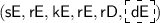
Definition. A ${\mathbb {Z}}_p$-linear predicate encoding for ${\mathsf {P}}: {\mathcal {X}}\times {\mathcal {Y}}\rightarrow \{0,1\}$ consists of five deterministic algorithms

$$ \begin{array}{lll} \mathsf {sE}: {\mathcal {X}}\times {\mathbb {Z}}_p^n \rightarrow {\mathbb {Z}}_p^{n_s} &{} &{} \qquad \mathsf {sD}: {\mathcal {X}}\times {\mathcal {Y}}\times {\mathbb {Z}}_p^{n_s} \rightarrow {\mathbb {Z}}_p \\ \mathsf {rE}: {\mathcal {Y}}\times {\mathbb {Z}}_p^n \rightarrow {\mathbb {Z}}_p^{n_r} &{} \qquad \mathsf {kE}: {\mathcal {Y}}\times {\mathbb {Z}}_p \rightarrow {\mathbb {Z}}_p^{n_r} &{} \qquad \mathsf {rD}: {\mathcal {X}}\times {\mathcal {Y}}\times {\mathbb {Z}}_p^{n_r} \rightarrow {\mathbb {Z}}_p \\ \end{array} $$

for some $n,n_s,n_r \in \mathbb {N}$ with the following features:  

(linearity). :

For all $(x,y) \in {\mathcal {X}}\times {\mathcal {Y}}$, $\mathsf {sE}(x,\cdot ), \mathsf {rE}(y,\cdot ), \mathsf {kE}(y,\cdot ), \mathsf {sD}(x,y,\cdot )$, $\mathsf {rD}(x,y,\cdot )$ are ${\mathbb {Z}}_p$-linear. A ${\mathbb {Z}}_p$-linear function $L : {\mathbb {Z}}_p^n \rightarrow {\mathbb {Z}}_p^{n'}$ can be encoded as a matrix $\mathbf {L}= (l_{i,j}) \in {\mathbb {Z}}_p^{n \times n'}$ such that

$$\begin{aligned} \textstyle L : (w_1,\ldots ,w_n) \mapsto (\sum _{i=1}^n l_{i1}w_i,\ldots ,\sum _{i=1}^n l_{in'} w_i). \end{aligned}$$

(5)

(restricted $\alpha$ -reconstruction). :

For all $(x,y) \in {\mathcal {X}}\times {\mathcal {Y}}$ such that ${\mathsf {P}}(x,y) = 1$, all $\mathbf {w}\in {\mathbb {Z}}_p^n$ and all $\alpha \in {\mathbb {Z}}_p$, we have

$$ \mathsf {sD}(x,y,\mathsf {sE}(x,\mathbf {w})) = \mathsf {rD}(x,y,\mathsf {rE}(y,\mathbf {w})) \quad \text{ and }\quad \mathsf {rD}(x,y,\mathsf {kE}(y,\alpha )) = \alpha . $$

( $\alpha$ -privacy). :

For all $(x,y) \in {\mathcal {X}}\times {\mathcal {Y}}$ such that ${\mathsf {P}}(x,y) = 0$ and all $\alpha \in {\mathbb {Z}}_p$, the following distributions are identical.

$$\begin{aligned}&\{x,y,\alpha ,\mathsf {sE}(x,\mathbf {w}),\mathsf {kE}(y,\alpha ) + \mathsf {rE}(y,\mathbf {w}) : \mathbf {w}\leftarrow {\mathbb {Z}}_p^n\} \quad \text{ and }\quad \\&\{x,y,\alpha ,\mathsf {sE}(x,\mathbf {w}), \mathsf {rE}(y,\mathbf {w}) : \mathbf {w}\leftarrow {\mathbb {Z}}_p^n\}. \end{aligned}$$

 

We call n the parameter size and use $|\mathsf {sE}|$ and $|\mathsf {rE}|$ to denote $n_s$ and $n_r$, respectively, which indicate the sizes of sender encodings and receiver encoding. We note that $|\mathsf {sE}|$ and $|\mathsf {rE}|$ may depend on x and y respectively. For all $x \in {\mathcal {X}}$, we define the distribution

$$ \mathsf {sE}(x) \,{:=}\, \{\mathsf {sE}(x,\mathbf {w}) : \mathbf {w}\leftarrow {\mathbb {Z}}_p^n\}. $$

More Notations and Useful Facts. Assume $s \in \{1,2,T\}$. We can naturally define a series of ${\mathbb {Z}}_p$-linear functions from $\mathbf {L}$ as follows:

$$\begin{aligned} \textstyle \begin{array}{rccc} L : &{} (G_s^k)^n &{} \rightarrow &{} (G_s^k)^{n'}\\ &{} ([\mathbf {w}_1]_s,\ldots ,[\mathbf {w}_n]_s) &{} \mapsto &{} (\prod _{i=1}^n [\mathbf {w}_i]^{l_{i1}}_s,\ldots ,\prod _{i=1}^n [\mathbf {w}_i]_s^{l_{in'}}) \\ \end{array} \end{aligned}$$

(6)

Because they essentially share the same structure (i.e., $\mathbf {L}$), we employ the same notation L. It should be clear from the context. Then we highlight three properties regarding functions L with respective to the same $\mathbf {L}$ as follows:  

( $L(\cdot )$ and pairing $e$ are commutative). :

For any $\mathbf {a},\mathbf {b}_1,\ldots ,\mathbf {b}_n \in {\mathbb {Z}}_p^k$, we have

$$\begin{aligned} e([\mathbf {a}]_1,L([\mathbf {b}_1]_2,\ldots ,[\mathbf {b}_n]_2))= & {} L(e([\mathbf {a}]_1,[\mathbf {b}_1]_2),\ldots ,e([\mathbf {a}]_1,[\mathbf {b}_n]_2)) \end{aligned}$$

(7)

$$\begin{aligned} e(L([\mathbf {b}_1]_1,\ldots ,[\mathbf {b}_n]_1),[\mathbf {a}]_2)= & {} L(e([\mathbf {b}_1]_1,[\mathbf {a}]_2),\ldots ,e([\mathbf {b}_n]_1,[\mathbf {a}]_2)) \end{aligned}$$

(8)

( $L(\cdot )$ and $[\cdot ]_s$ are commutative). :

For any $w_1,\ldots ,w_n \in {\mathbb {Z}}_p$, we have

$$\begin{aligned} L([w_1]_s,\ldots ,[w_n]_s) = [L(w_1,\ldots ,w_n)]_s. \end{aligned}$$

(9)

( $L(\cdot )$ and “exponentiation” are commutative). :

For any $\mathbf {w}\in {\mathbb {Z}}_p^n$ and $[\mathbf {a}]_s \in G_s^k$, we have

$$\begin{aligned}{}[\mathbf {a}]_s^{L(\mathbf {w})} = L([\mathbf {a}]^\mathbf {w}_s). \end{aligned}$$

(10)

 

Concrete Instantiations. As an example, we show the predicate encoding for equality predicate as below. This is the simplest encoding and extracted from classical Lewko-Waters IBE [LW10].

• (encoding for equality [LW10]). Let ${\mathcal {X}}= {\mathcal {Y}}= {\mathbb {Z}}_p$ and ${\mathsf {P}}(x,y) = 1$ iff $x = y$. Let $n = 2$ and $w_1,w_2 \leftarrow {\mathbb {Z}}_p$. Define

  $$ \begin{array}{lll} \mathsf {sE}(x,(w_1,w_2)) \,{:=}\, w_1 + x w_2 &{} &{} \qquad \mathsf {sD}(x,y,c) \,{:=}\, c \\ \mathsf {rE}(y,(w_1,w_2)) \,{:=}\, w_1 + y w_2 &{} \qquad \mathsf {kE}(y,\alpha ) \,{:=}\, \alpha &{} \qquad \mathsf {rD}(x,y,k) \,{:=}\, k \\ \end{array} $$

Here we have $|\mathsf {sE}| = |\mathsf {rE}| = 1$.

3 ABE with Tags from Predicate Encodings

3.1 Construction

Our generic tag-based ABE from predicate encodings is described below.

• $\mathsf {Setup}(1^\lambda ,{\mathsf {P}})$: Let n be parameter size of predicate encoding $(\mathsf {sE},\mathsf {rE},\mathsf {kE},\mathsf {sD},\mathsf {rD})$ for ${\mathsf {P}}$. We sample

  $$\begin{aligned} \mathbf {A}\leftarrow {\mathcal {D}}_k, \quad {\mathbf {W}}_1,\ldots ,{\mathbf {W}}_n,{\mathbf {W}}\leftarrow {\mathbb {Z}}_p^{(k+1)\times k}, \quad \mathbf {k}\leftarrow {\mathbb {Z}}_p^{k+1} \end{aligned}$$

  and output the master public and secret key pair

  $$\begin{aligned}&\textsf {mpk}\,{:=}\, \{[\mathbf {A}]_1, [{\mathbf {W}}_1^{\!\scriptscriptstyle {\top }}\mathbf {A}]_1,\ldots ,[{\mathbf {W}}_n^{\!\scriptscriptstyle {\top }}\mathbf {A}]_1, [{\mathbf {W}}^{\!\scriptscriptstyle {\top }}\mathbf {A}]_1, [\mathbf {k}^{\!\scriptscriptstyle {\top }}\mathbf {A}]_T\}\\&{\textsf {msk}}\,{:=}\, \{{\mathbf {W}}_1,\ldots ,{\mathbf {W}}_n,{\mathbf {W}};\; \mathbf {k}\}. \end{aligned}$$

• $\mathsf {Enc}(\textsf {mpk},x,m)$: On input $x \in {\mathcal {X}}$ and $m \in G_T$, pick $\mathbf {s}\leftarrow {\mathbb {Z}}_p^k$ and $\varvec{\tau }\leftarrow \mathsf {sE}(x)$. Output

  $$\begin{aligned} {\textsf {ct}}_x \,{:=}\, \left\{ \begin{array}{rcl} C_0 &{} {:=} &{} [\mathbf {A}\mathbf {s}]_1, \\ {\mathbf {C}}_1&{} {:=} &{}\mathsf {sE}(x,[{\mathbf {W}}_1^{\!\scriptscriptstyle {\top }}\mathbf {A}\mathbf {s}]_1,\ldots ,[{\mathbf {W}}_n^{\!\scriptscriptstyle {\top }}\mathbf {A}\mathbf {s}]_1) \cdot [{\mathbf {W}}^{\!\scriptscriptstyle {\top }}\mathbf {A}\mathbf {s}]_1^{\varvec{\tau }},\\ C&{} {:=} &{}[\mathbf {k}^{\!\scriptscriptstyle {\top }}\mathbf {A}\mathbf {s}]_T \cdot m, \ \varvec{\tau }\; \end{array}\right\} \end{aligned}$$

• ${\mathsf {KeyGen}}(\textsf {mpk},{\textsf {msk}},y)$: On input $y \in {\mathcal {Y}}$, pick $\mathbf {r}\leftarrow _{\textsc {r}}{\mathbb {Z}}_p^{k}$ and output

  $$\begin{aligned} {\textsf {sk}}_y \,{:=}\, \left\{ \begin{array}{rcl} K_0 &{} {:=} &{} [\mathbf {r}]_2, \\ {\mathbf {K}}_1 &{} {:=} &{} \mathsf {kE}(y,[\mathbf {k}]_2) \cdot \mathsf {rE}(y, [{\mathbf {W}}_1 \mathbf {r}]_2, \ldots , [{\mathbf {W}}_n \mathbf {r}]_2),\\ K_2 &{} {:=} &{} [{\mathbf {W}}\mathbf {r}]_2 \end{array}\right\} \end{aligned}$$

• ${\mathsf {Dec}}(\textsf {mpk},{\textsf {sk}}_{y}, {\textsf {ct}}_{x})$: Compute

  $$\begin{aligned} K \leftarrow e(C_0,\mathsf {rD}(x,y,{\mathbf {K}}_1)) \cdot e(C_0,K_2)^{\mathsf {sD}(x,y,\varvec{\tau })}/e(\mathsf {sD}(x,y,{\mathbf {C}}_1),K_0) \end{aligned}$$

  and recover the message as $m \leftarrow C/K\in G_T.$

Correctness. For all $(x,y) \in {\mathcal {X}}\times {\mathcal {Y}}$ with ${\mathsf {P}}(x,y) = 1$, we may use the following abbreviation

$$\begin{aligned} \begin{array}{c} \mathsf {sE}(x,\cdot ) = \mathsf {sE}(\cdot ),\ \mathsf {rE}(y,\cdot ) = \mathsf {rE}(\cdot ),\ \mathsf {kE}(y,\cdot ) = \mathsf {kE}(\cdot );\\ \mathsf {sD}(x,y,\cdot ) = \mathsf {sD}(\cdot ),\ \mathsf {rD}(x,y,\cdot ) = \mathsf {rD}(\cdot ) \end{array} \end{aligned}$$

and have

$$\begin{aligned} \begin{array}{rl} &{} e(C_0,\mathsf {rD}({\mathbf {K}}_1)) \cdot e(C_0,K_2)^{\mathsf {sD}(\varvec{\tau })} \\ {\mathop {=}\limits ^{(a)}} &{} e([\mathbf {A}\mathbf {s}]_1,\mathsf {rD}(\mathsf {kE}([\mathbf {k}]_2))) \cdot e([\mathbf {A}\mathbf {s}]_1,\mathsf {rD}(\mathsf {rE}([{\mathbf {W}}_1 \mathbf {r}]_2, \ldots , [{\mathbf {W}}_n \mathbf {r}]_2))) \cdot [\mathbf {s}^{\!\scriptscriptstyle {\top }}\mathbf {A}^{\!\scriptscriptstyle {\top }}{\mathbf {W}}\mathbf {r}]_T^{\mathsf {sD}(\varvec{\tau })} \\ {\mathop {=}\limits ^{(b)}} &{} \mathsf {rD}(\mathsf {kE}([\mathbf {s}^{\!\scriptscriptstyle {\top }}\mathbf {A}^{\!\scriptscriptstyle {\top }}\mathbf {k}]_T)) \cdot \mathsf {rD}(\mathsf {rE}([\mathbf {s}^{\!\scriptscriptstyle {\top }}\mathbf {A}^{\!\scriptscriptstyle {\top }}{\mathbf {W}}_1 \mathbf {r}]_T, \ldots , [\mathbf {s}^{\!\scriptscriptstyle {\top }}\mathbf {A}^{\!\scriptscriptstyle {\top }}{\mathbf {W}}_n \mathbf {r}]_T)) \cdot [\mathbf {s}^{\!\scriptscriptstyle {\top }}\mathbf {A}^{\!\scriptscriptstyle {\top }}{\mathbf {W}}\mathbf {r}]_T^{\mathsf {sD}(\varvec{\tau })} \\ {\mathop {=}\limits ^{(c)}} &{} [\mathsf {rD}(\mathsf {kE}(\mathbf {s}^{\!\scriptscriptstyle {\top }}\mathbf {A}^{\!\scriptscriptstyle {\top }}\mathbf {k}))]_T \cdot [\mathsf {rD}(\mathsf {rE}(\mathbf {s}^{\!\scriptscriptstyle {\top }}\mathbf {A}^{\!\scriptscriptstyle {\top }}{\mathbf {W}}_1 \mathbf {r}, \ldots , \mathbf {s}^{\!\scriptscriptstyle {\top }}\mathbf {A}^{\!\scriptscriptstyle {\top }}{\mathbf {W}}_n \mathbf {r}))]_T \cdot [\mathbf {s}^{\!\scriptscriptstyle {\top }}\mathbf {A}^{\!\scriptscriptstyle {\top }}{\mathbf {W}}\mathbf {r}]_T^{\mathsf {sD}(\varvec{\tau })} \\ {\mathop {=}\limits ^{(d)}} &{} [\mathbf {s}^{\!\scriptscriptstyle {\top }}\mathbf {A}^{\!\scriptscriptstyle {\top }}\mathbf {k}]_T \cdot [\mathsf {sD}(\mathsf {sE}(\mathbf {s}^{\!\scriptscriptstyle {\top }}\mathbf {A}^{\!\scriptscriptstyle {\top }}{\mathbf {W}}_1 \mathbf {r}, \ldots , \mathbf {s}^{\!\scriptscriptstyle {\top }}\mathbf {A}^{\!\scriptscriptstyle {\top }}{\mathbf {W}}_n \mathbf {r}))]_T \cdot [\mathbf {s}^{\!\scriptscriptstyle {\top }}\mathbf {A}^{\!\scriptscriptstyle {\top }}{\mathbf {W}}\mathbf {r}]_T^{\mathsf {sD}(\varvec{\tau })} \\ {\mathop {=}\limits ^{(e)}} &{} [\mathbf {s}^{\!\scriptscriptstyle {\top }}\mathbf {A}^{\!\scriptscriptstyle {\top }}\mathbf {k}]_T \cdot \mathsf {sD}(\mathsf {sE}([\mathbf {s}^{\!\scriptscriptstyle {\top }}\mathbf {A}^{\!\scriptscriptstyle {\top }}{\mathbf {W}}_1 \mathbf {r}]_T, \ldots , [\mathbf {s}^{\!\scriptscriptstyle {\top }}\mathbf {A}^{\!\scriptscriptstyle {\top }}{\mathbf {W}}_n \mathbf {r}]_T)) \cdot [\mathbf {s}^{\!\scriptscriptstyle {\top }}\mathbf {A}^{\!\scriptscriptstyle {\top }}{\mathbf {W}}\mathbf {r}]_T^{\mathsf {sD}(\varvec{\tau })} \\ {\mathop {=}\limits ^{(f)}} &{} [\mathbf {s}^{\!\scriptscriptstyle {\top }}\mathbf {A}^{\!\scriptscriptstyle {\top }}\mathbf {k}]_T \cdot e(\mathsf {sD}(\mathsf {sE}([{\mathbf {W}}^{\!\scriptscriptstyle {\top }}_1 \mathbf {A}\mathbf {s}]_1, \ldots , [{\mathbf {W}}^{\!\scriptscriptstyle {\top }}_n \mathbf {A}\mathbf {s}]_1)),[\mathbf {r}]_2) \cdot e([{\mathbf {W}}^{\!\scriptscriptstyle {\top }}\mathbf {A}\mathbf {s}]^{\mathsf {sD}(\varvec{\tau })}_1,[\mathbf {r}]_2) \\ {\mathop {=}\limits ^{(g)}} &{} [\mathbf {s}^{\!\scriptscriptstyle {\top }}\mathbf {A}^{\!\scriptscriptstyle {\top }}\mathbf {k}]_T \cdot e(\mathsf {sD}(\mathsf {sE}([{\mathbf {W}}^{\!\scriptscriptstyle {\top }}_1 \mathbf {A}\mathbf {s}]_1, \ldots , [{\mathbf {W}}^{\!\scriptscriptstyle {\top }}_n \mathbf {A}\mathbf {s}]_1)),[\mathbf {r}]_2) \cdot e(\mathsf {sD}([{\mathbf {W}}^{\!\scriptscriptstyle {\top }}\mathbf {A}\mathbf {s}]^{\varvec{\tau }}_1),[\mathbf {r}]_2) \\ {\mathop {=}\limits ^{(h)}} &{} [\mathbf {s}^{\!\scriptscriptstyle {\top }}\mathbf {A}^{\!\scriptscriptstyle {\top }}\mathbf {k}]_T \cdot e(\mathsf {sD}(\mathsf {sE}([{\mathbf {W}}^{\!\scriptscriptstyle {\top }}_1 \mathbf {A}\mathbf {s}]_1, \ldots , [{\mathbf {W}}^{\!\scriptscriptstyle {\top }}_n \mathbf {A}\mathbf {s}]_1) \cdot [{\mathbf {W}}^{\!\scriptscriptstyle {\top }}\mathbf {A}\mathbf {s}]_1^{\varvec{\tau }}),[\mathbf {r}]_2)\\ {\mathop {=}\limits ^{ {(h)}}} &{} [\mathbf {s}^{\!\scriptscriptstyle {\top }}\mathbf {A}^{\!\scriptscriptstyle {\top }}\mathbf {k}]_T \cdot e(\mathsf {sD}({\mathbf {C}}_1),K_0) \end{array} \end{aligned}$$

which is sufficient for the correctness. We list the properties and the facts justifying each (labelled) equality in Table 3.

Table 3. Properties and Facts for Correctness.

Security Result. We give the following main theorem stating that the above generic tag-based ABE scheme is adaptively secure under standard assumption in the standard model. The remaining of this section will be devoted to the proof of the main theorem.

Theorem 1

(Main Theorem). For any p.p.t. adversary ${\mathcal {A}}$ making at most q key extraction queries, there exists algorithms ${\mathcal {B}}_1,{\mathcal {B}}_2,{\mathcal {B}}_3$ such that

$$ \mathsf {Adv}^{\textsc {abe}}_{{\mathcal {A}}}(\lambda ) \le \mathsf {Adv}^{{\mathcal {D}}_k}_{{\mathcal {B}}_1}(\lambda ) + q \cdot \mathsf {Adv}^{{\mathcal {D}}_k}_{{\mathcal {B}}_2}(\lambda ) + q \cdot \mathsf {Adv}^{{\mathcal {D}}_k}_{{\mathcal {B}}_3}(\lambda ) + 2^{-\varOmega (\lambda )} $$

and $\max \{ \mathsf {Time}({\mathcal {B}}_1),\mathsf {Time}({\mathcal {B}}_2),\mathsf {Time}({\mathcal {B}}_3)\} \approx \mathsf {Time}({\mathcal {A}}) + q \cdot k^2 \cdot {{\mathrm{poly}}}(\lambda ,n)$.

3.2 Proving the Main Theorem: High-Level Roadmap

From a high level, the proof basically follows the common dual system methodology. We first define semi-functional distributions under the master public key

$$ \textsf {mpk}= \{[\mathbf {A}]_1, [{\mathbf {W}}_1^{\!\scriptscriptstyle {\top }}\mathbf {A}]_1,\ldots ,[{\mathbf {W}}_n^{\!\scriptscriptstyle {\top }}\mathbf {A}]_1, [{\mathbf {W}}^{\!\scriptscriptstyle {\top }}\mathbf {A}]_1, [\mathbf {k}^{\!\scriptscriptstyle {\top }}\mathbf {A}]_T\}. $$

where $(\mathbf {A},{\mathbf {a}^{\scriptscriptstyle {\perp }}}) \leftarrow {\mathcal {D}}_k, {\mathbf {W}}_1,\ldots ,{\mathbf {W}}_n,{\mathbf {W}}\leftarrow {\mathbb {Z}}_p^{(k+1)\times k}, \mathbf {k}\leftarrow {\mathbb {Z}}_p^{k+1}$ as follows.

(semi-functional ciphertext). A semi-functional ciphertext for target attribute $x^* \in {\mathcal {X}}$ and challenge message pair $(m^*_0,m^*_1) \in {\mathcal {M}}\times {\mathcal {M}}$ is defined as follows:

where $\mathbf {c}\leftarrow {\mathbb {Z}}_p^{k+1}$ and $\varvec{\tau }^* \leftarrow \mathsf {sE}(x^*)$.

(semi-functional secret key). A semi-functional secret key for policy $y \in {\mathcal {Y}}$ is defined as follows:

where $\alpha \leftarrow {\mathbb {Z}}_p$. Note that all semi-functional secret keys in the system will share the same $\alpha$.

Game Sequence. Our proof employs the following game sequence.

• $\mathsf {G}_0$ is the real security game defined as Sect. 2.1.

• $\mathsf {G}_1$ is identical to $\mathsf {G}_0$ except that the challenge ciphertext is semi-functional.

• $\mathsf {G}_{2.i}$ (for $i \in {[0,q]}$) is identical to $\mathsf {G}_1$ except that the first i key extraction queries are replied with semi-functional secret keys.

• $\mathsf {G}_3$ is identical to $\mathsf {G}_{2.q}$ except that the challenge ciphertext is a semi-functional ciphertext for random message $m^* \in {\mathcal {M}}$.

Roughly speaking, we are going to prove that

$$ \mathsf {G}_0 \ {\mathop {\approx }\limits ^{\text {lem}~4}} \ \mathsf {G}_1 \ = \ \mathsf {G}_{2.0} \ {\mathop {\approx }\limits ^{\text {sec}~3.3}} \ \mathsf {G}_{2.1} \ {\mathop {\approx }\limits ^{\text {sec}~3.3}} \ \cdots \ {\mathop {\approx }\limits ^{\text {sec}~3.3}} \ \mathsf {G}_{2.q} \ {\mathop {=}\limits ^{\text {lem}~5}} \ \mathsf {G}_3. $$

Here “$\approx$” indicates that two games are computationally indistinguishable while “=” means that they are statistically indistinguishable. Let $\mathsf {Adv}^{i.j}_{{\mathcal {A}}}(\lambda )$ be the advantage function of any p.p.t. adversary ${\mathcal {A}}$ making at most q key extraction queries in $\mathsf {G}_{i.j}$ with security parameter $\lambda$.

We begin with two simple lemmas. First, it is not hard to see that $\mathsf {G}_1$ and $\mathsf {G}_{2.0}$ are actually the same and we have the following lemma.

Lemma 2

( $\mathsf {G}_1 = \mathsf {G}_{2.0}$ ). For any adversary ${\mathcal {A}}$, we have $\mathsf {Adv}^{1}_{{\mathcal {A}}}(\lambda ) = \mathsf {Adv}^{2.0}_{{\mathcal {A}}}(\lambda )$.

Next, observe that the challenge ciphertext in the last game $\mathsf {G}_3$ is created without secret bit $\beta \in \{0,1\}$. In other words, the challenge ciphertext reveals nothing about $\beta$. Therefore adversary has no advantage in guessing $\beta$ and we have the lemma below.

Lemma 3

For any adversary ${\mathcal {A}}$, we have $\mathsf {Adv}^{3}_{{\mathcal {A}}}(\lambda ) = 0$.

Following Chen et al.’s proof [CGW15], we can prove Lemma 4 showing $\mathsf {G}_0 \ \approx \ \mathsf {G}_1$ and Lemma 5 showing $\mathsf {G}_{2.q} = \mathsf {G}_3$. Due to the lack of space, we omit the proofs.

Lemma 4

( $\mathsf {G}_0 \approx \mathsf {G}_1$ ). For any p.p.t. adversary ${\mathcal {A}}$ making at most q key extraction queries, there exists an algorithm ${\mathcal {B}}$ such that

$$ |\mathsf {Adv}^{0}_{{\mathcal {A}}}(\lambda ) - \mathsf {Adv}^{1}_{{\mathcal {A}}}(\lambda )| \ \le \ \mathsf {Adv}^{{\mathcal {D}}_k}_{{\mathcal {B}}}(\lambda ) + 1/p $$

and $\mathsf {Time}({\mathcal {B}}) \approx \mathsf {Time}({\mathcal {A}}) + q \cdot k^2 \cdot {{\mathrm{poly}}}(\lambda ,n)$.

Lemma 5

( $\mathsf {G}_{2.q} = \mathsf {G}_3$ ). For any adversary ${\mathcal {A}}$, we have

$$| \mathsf {Adv}^{2.q}_{{\mathcal {A}}}(\lambda ) - \mathsf {Adv}^{3}_{{\mathcal {A}}}(\lambda ) | = 1/p.$$

In order to complete the proof, we prove that $\mathsf {G}_{2.i}$ is indistinguishable with $\mathsf {G}_{2.i+1}$ for all $i \in [0,q-1]$. The details are deferred to the next subsection.

3.3 Proving the Theorem: Filling the Gap Between $\mathsf {G}_{2.i}$ and $\mathsf {G}_{2.i+1}$

This subsection proves the indistinguishability of $\mathsf {G}_{2.i}$ and $\mathsf {G}_{2.i+1}$. We introduce an auxiliary game sequence which is based on the proof idea from Jutla and Roy [JR13]. In particular, we need the following two auxiliary distributions.

(pesudo-normal secret key). A pseudo-normal secret key for policy $y \in {\mathcal {Y}}$ is defined as follows:

where $\hat{r} \leftarrow {\mathbb {Z}}_p$ and $\gamma _1,\ldots ,\gamma _n \leftarrow {\mathbb {Z}}_p$ are the random coins for tag $\varvec{\tau }^*$ in the challenge ciphertext. Recall that we compute $\varvec{\tau }^* = \mathsf {sE}(x^*,(\gamma _1,\ldots ,\gamma _n))$ for target attribute $x^*$.

(pesudo-semi-functional secret key). A pseudo-semi-functional secret key for policy $y \in {\mathcal {Y}}$ is defined as follows:

where $\hat{r} \in {\mathbb {Z}}_p$ and $\gamma _1,\ldots ,\gamma _n \in {\mathbb {Z}}_p$ are defined as before and $\alpha \in {\mathbb {Z}}_p$ is the one used in the semi-functional secret key.

We note that the random coins $\gamma _1,\ldots ,\gamma _n$ for $\varvec{\tau }^*$ are independent of $x^*$ and thus we can pick them at the very beginning and use them to create secret keys of these two forms at any point.

Game Sub-sequence. For each $i \in [0,q-1]$, we define

• $\mathsf {G}_{2.i.1}$ is identical to $\mathsf {G}_{2.i}$ except that the $i+1$st key extraction query y is answered with a pseudo-normal secret key.

• $\mathsf {G}_{2.i.2}$ is identical to $\mathsf {G}_{2.i.1}$ except that the $i+1$st key extraction query y is answered with a pseudo-semi-functional secret key.

With this sub-sequence, we will prove that

$$\begin{aligned} \mathsf {G}_{2.i} {\mathop {\approx }\limits ^{\text {lem}~6}} \mathsf {G}_{2.i.1} {\mathop {=}\limits ^{\text {lem}~8}} \mathsf {G}_{2.i.2} {\mathop {\approx }\limits ^{\text {lem}~7}} \mathsf {G}_{2.i+1}. \end{aligned}$$

We first prove Lemma 6 showing that $\mathsf {G}_{2.i} \ \approx \ \mathsf {G}_{2.i.1}$ and note that, following almost the same strategy, we can also prove that $\mathsf {G}_{2.i.2} \ \approx \ \mathsf {G}_{2.i+1}$. Hence we will show the corresponding result in Lemma 7 but omit the proof.

Lemma 6

( $\mathsf {G}_{2.i} \ \approx \ \mathsf {G}_{2.i.1}$ ). For any p.p.t. adversary ${\mathcal {A}}$ making at most q key extraction queries, there exists an algorithm ${\mathcal {B}}$ such that

$$ |\mathsf {Adv}^{2.i}_{{\mathcal {A}}}(\lambda ) - \mathsf {Adv}^{2.i.1}_{{\mathcal {A}}}(\lambda )| \ \le \ \mathsf {Adv}^{{\mathcal {D}}_k}_{{\mathcal {B}}}(\lambda ) $$

and $\mathsf {Time}({\mathcal {B}}) \approx \mathsf {Time}({\mathcal {A}}) + q \cdot k^2 \cdot {{\mathrm{poly}}}(\lambda ,n)$.

Proof

Given $(\,{\mathcal {G}},[{\mathbf {M}}]_2,[\mathbf {t}]_2 = [{\mathbf {M}}\mathbf {u}+ \mathbf {e}v]_2\,)$ where $\mathbf {u}\leftarrow {\mathbb {Z}}_p^k$, $\mathbf {e}= (0,\ldots ,0,1)^{\!\scriptscriptstyle {\top }}\in {\mathbb {Z}}_p^{k+1}$ and either $v \leftarrow {\mathbb {Z}}_p$ or $v = 0$, algorithm ${\mathcal {B}}$ works as follows:

 

Initialize. :

Sample $(\mathbf {A},{\mathbf {a}^{\scriptscriptstyle {\perp }}}) \leftarrow {\mathcal {D}}_{k}, \quad \mathbf {k}\leftarrow {\mathbb {Z}}_p^{k+1}$ and $\beta \leftarrow \{0,1\}.$ Pick

$$ \widetilde{{\mathbf {W}}}_1,\cdots ,\widetilde{{\mathbf {W}}}_n,\widetilde{{\mathbf {W}}} \leftarrow {\mathbb {Z}}_p^{(k+1)\times k} \quad \text{ and }\quad \gamma _1,\ldots ,\gamma _n \leftarrow {\mathbb {Z}}_p $$

and program “hidden parameter” $\gamma _1,\ldots ,\gamma _n$ into ${\mathbf {W}}_1,\ldots ,{\mathbf {W}}_n,{\mathbf {W}}$ as follows

$$ {\mathbf {W}}_1 = \widetilde{{\mathbf {W}}}_1 + \gamma _1 {\mathbf {V}},\ \ldots ,\ {\mathbf {W}}_n = \widetilde{{\mathbf {W}}}_n + \gamma _n {\mathbf {V}}, \quad {\mathbf {W}}= \widetilde{{\mathbf {W}}} - {\mathbf {V}}$$

where ${\mathbf {V}}= {\mathbf {a}^{\scriptscriptstyle {\perp }}}\cdot (\underline{{\mathbf {M}}}{\overline{{\mathbf {M}}}}^{-1}) \in {\mathbb {Z}}_p^{(k+1) \times k}$. One may check that all ${\mathbf {W}}_i$ and ${\mathbf {W}}$ are uniformly distributed over ${\mathbb {Z}}_p^{(k+1) \times k}$ as required. Due to the fact that $\mathbf {A}^{\!\scriptscriptstyle {\top }}{\mathbf {a}^{\scriptscriptstyle {\perp }}}= {\mathbf {0}}$, we can return the master public key as follows

$$ \textsf {mpk}= \{[\mathbf {A}]_1, [\widetilde{{\mathbf {W}}}_1^{\!\scriptscriptstyle {\top }}\mathbf {A}]_1,\ldots ,[\widetilde{{\mathbf {W}}}_n^{\!\scriptscriptstyle {\top }}\mathbf {A}]_1, [\widetilde{{\mathbf {W}}}^{\!\scriptscriptstyle {\top }}\mathbf {A}]_1, [\mathbf {k}^{\!\scriptscriptstyle {\top }}\mathbf {A}]_T\}. $$

We note that ${\mathcal {B}}$ can not compute ${\mathbf {V}}$ and thus does not know ${\mathbf {W}}_1,\ldots ,{\mathbf {W}}_n,{\mathbf {W}}$.

Challenge ciphertext. :

For target attribute $x^*$ and challenge message pair $(m^*_0,m^*_1)$, we sample $\mathbf {c}\leftarrow {\mathbb {Z}}_p^{k+1}$, compute tag $\varvec{\tau }^* = \mathsf {sE}(x^*,(\gamma _1,\ldots ,\gamma _n))$ using the “hidden parameter” and create the challenge ciphertext as follows

$$ \{[\mathbf {c}]_1, \mathsf {sE}(x^*,[\widetilde{{\mathbf {W}}}_1^{\!\scriptscriptstyle {\top }}\mathbf {c}]_1,\ldots ,[\widetilde{{\mathbf {W}}}_n^{\!\scriptscriptstyle {\top }}\mathbf {c}]_1) \cdot [\widetilde{{\mathbf {W}}}^{\!\scriptscriptstyle {\top }}\mathbf {c}]_1^{\varvec{\tau }^*}, [\mathbf {k}^{\!\scriptscriptstyle {\top }}\mathbf {c}]_T \cdot m^*_\beta ,\,\varvec{\tau }^*\} $$

Let $\mathbf {v}= \underline{{\mathbf {M}}}{\overline{{\mathbf {M}}}}^{-1}$, we show that

from the linearity of $\mathsf {sE}(x^*,\cdot )$ and

$$ \begin{array}{rcl} &{} &{} \mathsf {sE}(x^*,[\gamma _1 \mathbf {v}^{\!\scriptscriptstyle {\top }}{\mathbf {a}^{\scriptscriptstyle {\perp }}}^{\!\scriptscriptstyle {\top }}\mathbf {c}]_1,\ldots ,[\gamma _n \mathbf {v}^{\!\scriptscriptstyle {\top }}{\mathbf {a}^{\scriptscriptstyle {\perp }}}^{\!\scriptscriptstyle {\top }}\mathbf {c}]_1) \cdot [- \mathbf {v}^{\!\scriptscriptstyle {\top }}{\mathbf {a}^{\scriptscriptstyle {\perp }}}^{\!\scriptscriptstyle {\top }}\mathbf {c}]_1^{\varvec{\tau }^*} \quad \text {(the boxed part)}\\ =&{}&{} \mathsf {sE}(x^*,[\mathbf {v}^{\!\scriptscriptstyle {\top }}{\mathbf {a}^{\scriptscriptstyle {\perp }}}^{\!\scriptscriptstyle {\top }}\mathbf {c}]_1^{(\gamma _1,\ldots ,\gamma _n)}) \cdot [- \mathbf {v}^{\!\scriptscriptstyle {\top }}{\mathbf {a}^{\scriptscriptstyle {\perp }}}^{\!\scriptscriptstyle {\top }}\mathbf {c}]_1^{\varvec{\tau }^*} \\ =&{}&{} [\mathbf {v}^{\!\scriptscriptstyle {\top }}{\mathbf {a}^{\scriptscriptstyle {\perp }}}^{\!\scriptscriptstyle {\top }}\mathbf {c}]_1^{\mathsf {sE}(x^*,(\gamma _1,\ldots ,\gamma _n))} \cdot [\mathbf {v}^{\!\scriptscriptstyle {\top }}{\mathbf {a}^{\scriptscriptstyle {\perp }}}^{\!\scriptscriptstyle {\top }}\mathbf {c}]_1^{-\varvec{\tau }^*} = {\mathbf {0}}, \end{array} $$

where the first equality is mainly implied by Eqs. (3) and (4), and the second equality comes from the fact shown in Eq. (10). This is sufficient to see that our simulation is perfect.

Key extraction. :

We consider three cases: (1) For the first i queries y, we sample $\mathbf {r}' \leftarrow {\mathbb {Z}}_p^k$ and implicitly set

$$ \mathbf {r}= \overline{{\mathbf {M}}}\mathbf {r}' \in {\mathbb {Z}}_p^k. $$

The vector $\mathbf {r}$ here is uniformly distributed as required and we can compute $[\mathbf {r}]_2$ and simulate

$$ [{\mathbf {V}}\mathbf {r}]_2 = [{\mathbf {a}^{\scriptscriptstyle {\perp }}}\cdot (\underline{{\mathbf {M}}}\mathbf {r}')]_2. $$

These suffice for creating the secret key as

$$ \big \{ [\mathbf {r}]_2, \mathsf {kE}(y, [\mathbf {k}]_2 ) \cdot \mathsf {rE}(y, [\widetilde{{\mathbf {W}}}_1 \mathbf {r}]_2 \cdot [\gamma _1{\mathbf {V}}\mathbf {r}]_2, \ldots , [\widetilde{{\mathbf {W}}}_n \mathbf {r}]_2 \cdot [\gamma _n {\mathbf {V}}\mathbf {r}]_2), [\widetilde{{\mathbf {W}}}\mathbf {r}]_2 \cdot [-{\mathbf {V}}\mathbf {r}]_2 \big \} $$

because $\mathbf {k}$, $\widetilde{{\mathbf {W}}}_1,\ldots ,\widetilde{{\mathbf {W}}}_n,\widetilde{{\mathbf {W}}}$ and $\gamma _1,\ldots ,\gamma _n$ are all known to ${\mathcal {B}}$. (2) For the $i+1$st query y, we implicitly set

$$ \mathbf {r}= \overline{{\mathbf {M}}}\mathbf {u}= \overline{\mathbf {t}} \in {\mathbb {Z}}_p^k. $$

The vector $\mathbf {r}$ is distributed properly and $[\mathbf {r}]_2 = [\,\overline{\mathbf {t}}\,]_2$ can be simulated. Then we may produce the secret key as follows

$$ \left\{ \begin{array}{c} [\,\overline{\mathbf {t}}\,]_2,\ \mathsf {kE}(y, [\mathbf {k}]_2 ) \cdot \mathsf {rE}(y, [\,\widetilde{{\mathbf {W}}}_1 \overline{\mathbf {t}}\,]_2 \cdot [\,\gamma _1{\mathbf {a}^{\scriptscriptstyle {\perp }}}\underline{\mathbf {t}}\,]_2, \ldots , [\,\widetilde{{\mathbf {W}}}_n \overline{\mathbf {t}}\,]_2 \cdot [\,\gamma _n {\mathbf {a}^{\scriptscriptstyle {\perp }}}\underline{\mathbf {t}}\,]_2),\\ {[\,\widetilde{{\mathbf {W}}} \overline{\mathbf {t}}\,]_2 \cdot [\,- {\mathbf {a}^{\scriptscriptstyle {\perp }}}\underline{\mathbf {t}}\,]_2} \end{array} \right\} . $$

(3) For the remaining $q - i - 1$ queries, we may work just as in the first case except that we employ $\mathbf {k}+\alpha {\mathbf {a}^{\scriptscriptstyle {\perp }}}$ in the place of $\mathbf {k}$.

Finalize.:

Output 1 when $\beta = \beta '$ and 0 otherwise.  

Observe that, in the reply to the $i+1$st key extraction query, we have

$$ {\mathbf {a}^{\scriptscriptstyle {\perp }}}\underline{\mathbf {t}}= {\mathbf {a}^{\scriptscriptstyle {\perp }}}(\underline{{\mathbf {M}}}\mathbf {u}+ v) = {\mathbf {a}^{\scriptscriptstyle {\perp }}}(\underline{{\mathbf {M}}}{\overline{{\mathbf {M}}}}^{-1}) (\overline{{\mathbf {M}}}\mathbf {u}) + {\mathbf {a}^{\scriptscriptstyle {\perp }}}v = {\mathbf {V}}\overline{\mathbf {t}} + {\mathbf {a}^{\scriptscriptstyle {\perp }}}v. $$

Therefore we have

$$ \begin{array}{rcl} &{} &{} \mathsf {kE}(y, [\mathbf {k}]_2 ) \cdot \mathsf {rE}(y, [\,\widetilde{{\mathbf {W}}}_1 \overline{\mathbf {t}}\,]_2 \cdot [\,\gamma _1{\mathbf {a}^{\scriptscriptstyle {\perp }}}\underline{\mathbf {t}}\,]_2, \ldots , [\,\widetilde{{\mathbf {W}}}_n \overline{\mathbf {t}}\,]_2 \cdot [\,\gamma _n {\mathbf {a}^{\scriptscriptstyle {\perp }}}\underline{\mathbf {t}}\,]_2) \\ =&{}&{} \mathsf {kE}(y, [\mathbf {k}]_2 ) \cdot \mathsf {rE}(y, [\,{\mathbf {W}}_1 \mathbf {r}\,]_2 \cdot [\,\gamma _1{\mathbf {a}^{\scriptscriptstyle {\perp }}}v\,]_2, \ldots , [\,{\mathbf {W}}_n \mathbf {r}\,]_2 \cdot [\,\gamma _n {\mathbf {a}^{\scriptscriptstyle {\perp }}}v\,]_2)\\ =&{}&{} \mathsf {kE}(y, [\mathbf {k}]_2 ) \cdot \mathsf {rE}(y, [\,{\mathbf {W}}_1 \mathbf {r}\,]_2, \ldots , [\,{\mathbf {W}}_n \mathbf {r}\,]_2 ) \cdot \mathsf {rE}(y, [\,\gamma _1{\mathbf {a}^{\scriptscriptstyle {\perp }}}v\,]_2, \ldots , [\,\gamma _n {\mathbf {a}^{\scriptscriptstyle {\perp }}}v\,]_2) \\ =&{}&{} \mathsf {kE}(y, [\mathbf {k}]_2 ) \cdot \mathsf {rE}(y, [\,{\mathbf {W}}_1 \mathbf {r}\,]_2, \ldots , [\,{\mathbf {W}}_n \mathbf {r}\,]_2 ) \cdot \mathsf {rE}(y, [\,{\mathbf {a}^{\scriptscriptstyle {\perp }}}v\,]_2^{(\gamma _1,\ldots ,\gamma _n)}) \\ =&{}&{} \mathsf {kE}(y, [\mathbf {k}]_2 ) \cdot \mathsf {rE}(y, [\,{\mathbf {W}}_1 \mathbf {r}\,]_2, \ldots , [\,{\mathbf {W}}_n \mathbf {r}\,]_2 ) \cdot [\,{\mathbf {a}^{\scriptscriptstyle {\perp }}}v \,]_2^{\mathsf {sE}(y,\gamma _1,\ldots ,\gamma _n)} \\ &{} &{} [\,\widetilde{{\mathbf {W}}} \overline{\mathbf {t}}\,]_2 \cdot [\,- {\mathbf {a}^{\scriptscriptstyle {\perp }}}\underline{\mathbf {t}}\,]_2 \\ =&{}&{} [\,{\mathbf {W}}\mathbf {r}\,]_2 \cdot [\, - {\mathbf {a}^{\scriptscriptstyle {\perp }}}v\,]_2 \\ =&{}&{} [\,{\mathbf {W}}\mathbf {r}\,]_2 \cdot [\, {\mathbf {a}^{\scriptscriptstyle {\perp }}}v\,]_2^{-1} \end{array} $$

It is now clear that the simulation is identical to $\mathsf {G}_{2.i}$ when $v = 0$; and if v is a random element in ${\mathbb {Z}}_p$, the simulation is identical to $\mathsf {G}_{2.i.1}$ where $\hat{r} = v$.    $\square$

Lemma 7

( $\mathsf {G}_{2.i.2} \ \approx \ \mathsf {G}_{2.i+1}$ ). For any p.p.t. adversary ${\mathcal {A}}$ making at most q key extraction queries, there exists an algorithm ${\mathcal {B}}$ such that

$$ |\mathsf {Adv}^{2.i.2}_{{\mathcal {A}}}(\lambda ) - \mathsf {Adv}^{2.i+1}_{{\mathcal {A}}}(\lambda )| \ \le \ \mathsf {Adv}^{{\mathcal {D}}_k}_{{\mathcal {B}}}(\lambda ) $$

and $\mathsf {Time}({\mathcal {B}}) \approx \mathsf {Time}({\mathcal {A}}) + q \cdot k^2 \cdot {{\mathrm{poly}}}(\lambda ,n)$.

Proof

The proof is similar to that for Lemma 6.    $\square$

We complete the proof by proving Lemma 8 which states that $\mathsf {G}_{2.i.1}$ and $\mathsf {G}_{2.i.2}$ are statistically indistinguishable. This is derived from the $\alpha$-privacy of predicate encodings.

Lemma 8

( $\mathsf {G}_{2.i.1} = \mathsf {G}_{2.i.2}$ ). For any adversary ${\mathcal {A}}$, we have

$$ \mathsf {Adv}^{2.i.1}_{{\mathcal {A}}}(\lambda ) = \mathsf {Adv}^{2.i.2}_{{\mathcal {A}}}(\lambda ). $$

Proof

We prove the lemma for any fixed

• $(\mathbf {A},{\mathbf {a}^{\scriptscriptstyle {\perp }}}) \leftarrow {\mathcal {D}}_k$, ${\mathbf {W}}_1,\ldots ,{\mathbf {W}}_n,{\mathbf {W}}\leftarrow {\mathbb {Z}}_p^{(k+1) \times k}$, $\mathbf {k}\leftarrow {\mathbb {Z}}_p^{k+1}$, $\beta \leftarrow \{0,1\}$;

• random coin $\mathbf {c}\leftarrow {\mathbb {Z}}_p^{k+1}$ for semi-functional challenge ciphertext ${\textsf {ct}}^*$;

• $\alpha \leftarrow {\mathbb {Z}}_p$, random coin $\mathbf {r}\leftarrow {\mathbb {Z}}_p^k$ for each key extraction query and the extra random coin $\hat{r} \leftarrow {\mathbb {Z}}_p$ for the $i+1$st one.

Let ${\textsf {sk}}_y^{(b)}$ be the reply to the $i+1$st key extraction query y in $\mathsf {G}_{2.i.b}$ ($b = 1,2$) and ${\textsf {ct}}^*$ is the challenge ciphertext for target attribute $x^*$. It is sufficient to show

$$ \{({\textsf {sk}}_y^{(1)},{\textsf {ct}}^*)\} = \{({\textsf {sk}}_y^{(2)},{\textsf {ct}}^*)\} $$

where the probability space is defined by $\gamma _1,\ldots ,\gamma _n \leftarrow {\mathbb {Z}}_p$. In fact, we can further reduce to the claim that

$$\begin{aligned}&\{\mathsf {kE}(y,[\alpha {\mathbf {a}^{\scriptscriptstyle {\perp }}}]_2) \cdot [{\mathbf {a}^{\scriptscriptstyle {\perp }}}\hat{r}]_2^{\mathsf {rE}(y,\gamma _1,\ldots ,\gamma _n)},\quad \mathsf {sE}(x^*,\gamma _1,\ldots ,\gamma _n)\}\ \text { and } \\&\{[{\mathbf {a}^{\scriptscriptstyle {\perp }}}\hat{r}]_2^{\mathsf {rE}(y,\gamma _1,\ldots ,\gamma _n)},\quad \mathsf {sE}(x^*,\gamma _1,\ldots ,\gamma _n)\} \end{aligned}$$

are statistically close over the same probability space as before. One can rewrite the first distribution as

$$ \{[{\mathbf {a}^{\scriptscriptstyle {\perp }}}\hat{r}]_2^{\mathsf {kE}(y,\alpha /\hat{r}) + \mathsf {rE}(y,\gamma _1,\ldots ,\gamma _n)},\quad \mathsf {sE}(x^*,\gamma _1,\ldots ,\gamma _n)\}. $$

which is statistically close to the second one by the $\alpha$-privacy of predicate encoding. This readily proves the lemma.    $\square$

4 Tag-Based ABE with Weak Attribute-Hiding Property

This section shows that our framework (presented in Sect. 3) is compatible with the attribute-hiding predicate encoding [CGW15]. This means that our framework can derive a series of attribute-hiding ABE with tag.

4.1 Preliminaries

Definition. We may call an ABE with (weak) attribute-hiding the predicate encryption (PE for short). A PE scheme is also defined by four p.p.t algorithms $\mathsf {Setup},{\mathsf {KeyGen}},\mathsf {Enc},{\mathsf {Dec}}$ as in Sect. 2, but the security is defined in a slightly different way. For all adversary ${\mathcal {A}}$, define the advantage function $\mathsf {Adv}^{\textsc {pe}}_{{\mathcal {A}}}(\lambda )$ as

$$ \mathsf {Adv}^{\textsc {pe}}_{{\mathcal {A}}}(\lambda ) = \left| \Pr \left[ \beta = \beta ' \left| \begin{array}{c} (\textsf {mpk},{\textsf {msk}}) \leftarrow \mathsf {Setup}(1^\lambda ,{\mathsf {P}}),\ \beta \leftarrow \{0,1\}\\ (x^*_0,x^*_1,m_0^*,m_1^*) \leftarrow {\mathcal {A}}^{{\mathsf {KeyGen}}(\textsf {mpk},{\textsf {msk}},\cdot )}(\textsf {mpk})\\ {\textsf {ct}}^* \leftarrow \mathsf {Enc}(\textsf {mpk},x^*_\beta ,m^*_\beta )\\ \beta ' \leftarrow {\mathcal {A}}^{{\mathsf {KeyGen}}(\textsf {mpk},{\textsf {msk}},\cdot )}(\textsf {mpk},{\textsf {ct}}^*) \end{array} \right. \right] - \frac{1}{2} \right| . $$

A PE scheme is said to be adaptively secure and weakly attribute-hiding if $\mathsf {Adv}^{\textsc {pe}}_{{\mathcal {A}}}(\lambda )$ is negligible in $\lambda$ and ${\mathsf {P}}(x^*_0,y) = {\mathsf {P}}(x^*_1,y) = 0$ holds for each query y sent to oracle ${\mathsf {KeyGen}}(\textsf {mpk},{\textsf {msk}},\cdot )$ for all p.p.t. adversary ${\mathcal {A}}$.

Attribute-hiding Predicate Encoding. A ${\mathbb {Z}}_p$-linear predicate encoding $(\mathsf {sE},\mathsf {rE},\mathsf {kE},\mathsf {sD},\mathsf {rD})$ for ${\mathsf {P}}: {\mathcal {X}}\times {\mathcal {Y}}\rightarrow \{0,1\}$ is attribute-hiding [CGW15] if it has the following two additional properties:  

( x -oblivious $\alpha$-reconstruction). :

$\mathsf {sD}(x,y,\cdot )$ and $\mathsf {rD}(x,y,\cdot )$ are independent of x.

(attribute-hiding). :

For all $(x,y) \in {\mathcal {X}}\times {\mathcal {Y}}$ such that ${\mathsf {P}}(x,y) = 0$ , the following distributions are identical.

$$ \big \{x,y,\mathsf {sE}(x,\mathbf {w}), \mathsf {rE}(y,\mathbf {w}) : \mathbf {w}\leftarrow {\mathbb {Z}}_p^n\big \} \quad \text{ and }\quad \big \{x,y,\mathbf {r}: \mathbf {r}\leftarrow {\mathbb {Z}}_p^{|\mathsf {sE}|+|\mathsf {rE}|}\big \}. $$

 

4.2 Construction and Security Analysis

Assuming an attribute-hiding predicate encoding, we can construct a predicate encryption with tag as in Sect. 3.1. Technically we prove the following theorem stating that the generic tag-based PE scheme is adaptively secure and weakly attribute-hiding under standard assumption in the standard model.

Theorem 2

(Weak AH). For any p.p.t. adversary ${\mathcal {A}}$ making at most q key extraction queries, there exists algorithms ${\mathcal {B}}_1,{\mathcal {B}}_2,{\mathcal {B}}_3$ such that

$$ \mathsf {Adv}^{\textsc {pe}}_{{\mathcal {A}}}(\lambda ) \le \mathsf {Adv}^{{\mathcal {D}}_k}_{{\mathcal {B}}_1}(\lambda ) + q \cdot \mathsf {Adv}^{{\mathcal {D}}_k}_{{\mathcal {B}}_2}(\lambda ) + q \cdot \mathsf {Adv}^{{\mathcal {D}}_k}_{{\mathcal {B}}_3}(\lambda ) + 2^{-\varOmega (\lambda )} $$

and $\max \{\mathsf {Time}({\mathcal {B}}_1),\mathsf {Time}({\mathcal {B}}_2),\mathsf {Time}({\mathcal {B}}_3)\} \approx \mathsf {Time}({\mathcal {A}}) + q \cdot k^2 \cdot {{\mathrm{poly}}}(\lambda ,n)$.

Proof Overview. We prove the theorem using almost the same game sequence as described in Sects. 3.2 and 3.3. We just describe the differences between them. Firstly, the challenge ciphertext will be generated for identity $x^*_\beta$. Secondly, we need to re-define pseudo-semi-functional secret keys and semi-functional secret keys as follows.

(pesudo-semi-functional secret key). A pseudo-semi-functional secret key for policy $y \in {\mathcal {Y}}$ is defined as follows:

where $\hat{r} \in {\mathbb {Z}}_p$, $\gamma _1,\ldots ,\gamma _n \in {\mathbb {Z}}_p$, $\alpha \in {\mathbb {Z}}_p$ are defined as before and $\hat{u}_1,\ldots ,\hat{u}_n \leftarrow {\mathbb {Z}}_p$ are fresh for each pseudo-semi-functional secret key.

(semi-functional secret key). A semi-functional secret key for policy $y \in {\mathcal {Y}}$ is defined as follows:

where $\alpha \in {\mathbb {Z}}_p$ are defined as before and $\hat{u}_1,\ldots ,\hat{u}_n \leftarrow {\mathbb {Z}}_p$ are fresh for each semi-functional secret key.

Finally, we add an additional game $\mathsf {G}_4$ shown below. Its preceding game $\mathsf {G}_3$ (the final game in the previous game sequence) is restated so as to emphasize the difference between them.

• $\mathsf {G}_3$ is identical to $\mathsf {G}_{2.q}$ except that the challenge ciphertext is a semi-functional ciphertext for attribute $x^*_\beta$ and .

• $\mathsf {G}_4$ is identical to $\mathsf {G}_3$ except that the challenge ciphertext is a semi-functional ciphertext for and random message $m^* \in {\mathcal {M}}$.

With the extended game sequence, we will prove that

where “$\mathsf {G}_{2.i} \approx \mathsf {G}_{2.i+1}$” for all $i \in [0,q]$ will be proved using the game sub-sequence

Because of the similarity of game sequences, most lemmas we have presented in Sects. 3.2 and 3.3 still hold and can be proved in the same way. Due to the lack of space, we omit them. The proofs of “$\mathsf {G}_3 = \mathsf {G}_4$” and “$\mathsf {G}_{2.i.1} = \mathsf {G}_{2.i.2}$” (the boxed parts) mainly follow [CGW15] and our proof in previous section.

Finally, we point out the fact: The challenge ciphertext in $\mathsf {G}_3$ still leaks information of $\beta \in \{0,1\}$ via $x^*_\beta$, but such a dependence is removed in $\mathsf {G}_4$. Therefore $\mathsf {Adv}^{4}_{{\mathcal {A}}}(\lambda ) = 0$ for any ${\mathcal {A}}$.

5 New Tag-Based ABE

In this section we will exhibit two tag-based ABE for boolean span program derived from our generic tag-based ABE and two concrete encodings in [CGW15].

Boolean Span Program. Assume $n \in \mathbb {N}$. Let [n] be the attribute universe. A span program over [n] is defined by $({\mathbf {M}},\rho )$ where ${\mathbf {M}}\in {\mathbb {Z}}_p^{\ell \times \ell '}$ and $\rho : [\ell ] \rightarrow [n]$. We use ${\mathbf {M}}_i$ to denote the ith row of ${\mathbf {M}}$. For an input $\mathbf {x}= (x_1,\ldots ,x_n) \in \{0,1\}^n$, we say

where $\mathbf {1}= (1,0,\ldots ,0) \in {\mathbb {Z}}_p^{1 \times \ell '}$ and ${\mathbf {M}}_\mathbf {x}= \{\,{\mathbf {M}}_j : x_{\rho (j)} = 1 \,\}$. In this case one can efficiently find coefficients $\omega _1,\ldots ,\omega _\ell \in {\mathbb {Z}}_p$ such that

$$\textstyle \sum _{j\;:\;x_{\rho (j) = 1}} \omega _j {\mathbf {M}}_j = \mathbf {1}. $$

Here we will assume $n = \ell$ and $\rho$ is an identity map following [CGW15].

5.1 Key-Policy Construction

The corresponding predicate is defined as

where $\mathbf {x}\in {\mathcal {X}}= \{0,1\}^\ell$ and ${\mathbf {M}}\in {\mathcal {Y}}= {\mathbb {Z}}_p^{\ell \times \ell '}$. Our concrete KP-ABE scheme is described below:

• $\mathsf {Setup}(1^\lambda ,1^\ell )$: Sample

  $$ \mathbf {A}\leftarrow {\mathcal {D}}_k, \quad {\mathbf {W}}_1,\ldots ,{\mathbf {W}}_\ell ,{\mathbf {U}}_2,\ldots ,{\mathbf {U}}_{\ell '},{\mathbf {W}}\leftarrow {\mathbb {Z}}_p^{(k+1)\times k}, \quad \mathbf {k}\leftarrow {\mathbb {Z}}_p^{k+1} $$

  and output

  $$ \begin{array}{rcl} \textsf {mpk}&{} \,{:=}\, &{} \{[\mathbf {A}]_1, [{\mathbf {W}}_1^{\!\scriptscriptstyle {\top }}\mathbf {A}]_1,\ldots ,[{\mathbf {W}}_\ell ^{\!\scriptscriptstyle {\top }}\mathbf {A}]_1, [{\mathbf {W}}^{\!\scriptscriptstyle {\top }}\mathbf {A}]_1, [\mathbf {k}^{\!\scriptscriptstyle {\top }}\mathbf {A}]_T\} \\ {\textsf {msk}}&{} \,{:=}\, &{} \{{\mathbf {W}}_1,\ldots ,{\mathbf {W}}_\ell ,{\mathbf {U}}_2,\ldots ,{\mathbf {U}}_{\ell '},{\mathbf {W}};\; \mathbf {k}\} \end{array} $$

• $\mathsf {Enc}(\textsf {mpk},\mathbf {x},m)$: On input $\mathbf {x}\in \{0,1\}^\ell$ and $m \in G_T$, pick $\mathbf {s}\leftarrow {\mathbb {Z}}_p^k$ and $w_1,\ldots ,w_\ell \leftarrow {\mathbb {Z}}_p$. Output

  $$\begin{aligned} {\textsf {ct}}_\mathbf {x}\,{:=}\, \left\{ \begin{array}{rcl} C_0 &{} {:=} &{} [\mathbf {A}\mathbf {s}]_1, \\ C_1 &{} {:=} &{} [x_1 ({\mathbf {W}}_1 + w_1 {\mathbf {W}}) ^{\!\scriptscriptstyle {\top }}\mathbf {A}\mathbf {s}]_1,\\ &{} \vdots &{}\\ C_\ell &{} {:=} &{} [x_\ell ({\mathbf {W}}_\ell + w_\ell {\mathbf {W}})^{\!\scriptscriptstyle {\top }}\mathbf {A}\mathbf {s}]_1,\\ C &{} {:=} &{} [\mathbf {k}^{\!\scriptscriptstyle {\top }}\mathbf {A}\mathbf {s}]_T \cdot m,\\ \varvec{\tau }&{} {:=} &{} ( \tau _1 \,{:=}\, x_1 w_1, \ldots , \tau _\ell \,{:=}\, x_\ell w_\ell ) \end{array}\right\} \in G_1^{k+1} \times (G_1^{k})^{\ell } \times G_T \times {\mathbb {Z}}_p^\ell \end{aligned}$$

• ${\mathsf {KeyGen}}(\textsf {mpk},{\textsf {msk}},{\mathbf {M}})$: On input ${\mathbf {M}}\in {\mathbb {Z}}_p^{\ell \times \ell '}$, pick $\mathbf {r}\leftarrow _{\textsc {r}}{\mathbb {Z}}_p^{k}$ and output

  $$\begin{aligned} {\textsf {sk}}_{\mathbf {M}}\,{:=}\, \left\{ \begin{array}{rcl} K_0 &{} {:=} &{} [\mathbf {r}]_2,\\ K_1 &{} {:=} &{} [(\mathbf {k}||{\mathbf {U}}_2\mathbf {r}||\cdots ||{\mathbf {U}}_{\ell '}\mathbf {r}){\mathbf {M}}_1^{\!\scriptscriptstyle {\top }}+ {\mathbf {W}}_1 \mathbf {r}]_2 ,\\ &{} \vdots &{}\\ K_\ell &{} {:=} &{} [(\mathbf {k}||{\mathbf {U}}_2\mathbf {r}||\cdots ||{\mathbf {U}}_{\ell '}\mathbf {r}){\mathbf {M}}_\ell ^{\!\scriptscriptstyle {\top }}+ {\mathbf {W}}_\ell \mathbf {r}]_2 ,\\ K_t &{} {:=} &{} [{\mathbf {W}}\mathbf {r}]_2 \end{array}\right\} \in G_2^{k} \times (G_2^{k+1})^{\ell } \times G_2^{k+1} \end{aligned}$$

• ${\mathsf {Dec}}(\textsf {mpk},{\textsf {sk}}_{{\mathbf {M}}}, {\textsf {ct}}_{\mathbf {x}})$: Find out $\omega _1,\ldots ,\omega _\ell \in {\mathbb {Z}}_p$ such that $\sum _{j:x_j = 1} \omega _j {\mathbf {M}}_j = \mathbf {1}$ and compute

  $$ K \leftarrow e(C_0,\prod _{j:x_j = 1}(K_j \cdot K_t^{\tau _j})^{\omega _j}) \cdot e(\prod _{j:x_j = 1} C_j^{-\omega _j},K_0) $$

  Recover the message as $m \leftarrow C/K \in G_T$.

5.2 Ciphertext-Policy Construction

The corresponding predicate is defined as

where ${\mathbf {M}}\in {\mathcal {X}}= {\mathbb {Z}}_p^{\ell \times \ell '}$ and $\mathbf {x}\in {\mathcal {Y}}= \{0,1\}^\ell$. Our concrete CP-ABE scheme is described below:

• $\mathsf {Setup}(1^\lambda ,1^\ell )$: Sample

  $$ \mathbf {A}\leftarrow {\mathcal {D}}_k, \quad {\mathbf {W}}_1,\ldots ,{\mathbf {W}}_\ell , {\mathbf {V}}, {\mathbf {W}}\leftarrow {\mathbb {Z}}_p^{(k+1)\times k}, \quad \mathbf {k}\leftarrow {\mathbb {Z}}_p^{k+1} $$

  and output

  $$ \begin{array}{rcl} \textsf {mpk}&{} \,{:=}\, &{} \{[\mathbf {A}]_1, [{\mathbf {W}}_1^{\!\scriptscriptstyle {\top }}\mathbf {A}]_1,\ldots ,[{\mathbf {W}}_\ell ^{\!\scriptscriptstyle {\top }}\mathbf {A}]_1, [{\mathbf {V}}^{\!\scriptscriptstyle {\top }}\mathbf {A}]_1, [{\mathbf {W}}^{\!\scriptscriptstyle {\top }}\mathbf {A}]_1, [\mathbf {k}^{\!\scriptscriptstyle {\top }}\mathbf {A}]_T\} \\ {\textsf {msk}}&{} \,{:=}\, &{} \{{\mathbf {W}}_1,\ldots ,{\mathbf {W}}_\ell ,{\mathbf {V}},{\mathbf {W}};\; \mathbf {k}\} \end{array} $$

• $\mathsf {Enc}(\textsf {mpk},{\mathbf {M}},m)$: On input ${\mathbf {M}}\in {\mathbb {Z}}_p^{\ell \times \ell '}$ and $m \in G_T$, pick $\mathbf {s}\leftarrow {\mathbb {Z}}_p^k$ and

  $$ w_1,\ldots ,w_\ell \leftarrow {\mathbb {Z}}_p,\ v \leftarrow {\mathbb {Z}}_p, \ \mathbf {u}\leftarrow {\mathbb {Z}}_p^{\ell '-1}, \ {\mathbf {U}}_2,\ldots ,{\mathbf {U}}_{\ell '} \leftarrow {\mathbb {Z}}_p^{(k+1) \times k}. $$

  Output

  $$\begin{aligned}&{\textsf {ct}}_{\mathbf {M}}\,{:=}\, \\&\left\{ \begin{array}{rcl} C_0 &{}:=&{} [\mathbf {A}\mathbf {s}]_1, \\ C_1 &{}:=&{} [({\mathbf {W}}_1 + w_1 {\mathbf {W}})^{\!\scriptscriptstyle {\top }}\mathbf {A}\mathbf {s}+ (({\mathbf {V}}+ v{\mathbf {W}})^{\!\scriptscriptstyle {\top }}\mathbf {A}\mathbf {s}||{\mathbf {U}}_2^{\!\scriptscriptstyle {\top }}\mathbf {A}\mathbf {s}||\cdots ||{\mathbf {U}}_{\ell '}^{\!\scriptscriptstyle {\top }}\mathbf {A}\mathbf {s}) {\mathbf {M}}_1^{\!\scriptscriptstyle {\top }}]_1,\\ &{}\vdots &{}\\ C_\ell &{}:=&{} [({\mathbf {W}}_\ell + w_\ell {\mathbf {W}})^{\!\scriptscriptstyle {\top }}\mathbf {A}\mathbf {s}+ (({\mathbf {V}}+ v{\mathbf {W}})^{\!\scriptscriptstyle {\top }}\mathbf {A}\mathbf {s}||{\mathbf {U}}_2^{\!\scriptscriptstyle {\top }}\mathbf {A}\mathbf {s}||\cdots ||{\mathbf {U}}_{\ell '}^{\!\scriptscriptstyle {\top }}\mathbf {A}\mathbf {s}) {\mathbf {M}}_\ell ^{\!\scriptscriptstyle {\top }}]_1,\\ C &{}:= &{} [\mathbf {k}^{\!\scriptscriptstyle {\top }}\mathbf {A}\mathbf {s}]_T \cdot m, \\ \varvec{\tau }&{}:= &{} (\tau _1 := w_1 + {\mathbf {M}}_1 \left( {\begin{matrix}v\\ \mathbf {u}\\ \end{matrix}}\right) ,\; \ldots ,\; \tau _\ell := w_\ell + {\mathbf {M}}_\ell \left( {\begin{matrix}v\\ \mathbf {u}\\ \end{matrix}}\right) ) \end{array}\right\} \\&\qquad \qquad \qquad \qquad \qquad \in G_1^{k+1} \times (G_1^{k})^{\ell } \times G_T \times {\mathbb {Z}}_p^\ell \end{aligned}$$

• ${\mathsf {KeyGen}}(\textsf {mpk},{\textsf {msk}},\mathbf {x})$: On input $\mathbf {x}\in \{0,1\}^\ell$, pick $\mathbf {r}\leftarrow _{\textsc {r}}{\mathbb {Z}}_p^{k}$ and output

  $$\begin{aligned} {\textsf {sk}}_\mathbf {x}:= \left\{ \begin{array}{rcl} K_0 &{}:=&{} [\mathbf {r}]_2,\\ K_1 &{}:=&{} [x_1 {\mathbf {W}}_1 \mathbf {r}]_2 \\ &{}\vdots &{}\\ K_\ell &{}:=&{} [x_\ell {\mathbf {W}}_\ell \mathbf {r}]_2 \\ K_{\ell +1} &{}:=&{} [\mathbf {k}+ {\mathbf {V}}\mathbf {r}]_2 \\ K_t &{}:=&{} [{\mathbf {W}}\mathbf {r}]_2 \end{array} \right\} \in G_2^{k} \times (G_2^{k+1})^{\ell +1} \times G_2^{k+1} \end{aligned}$$

• ${\mathsf {Dec}}(\textsf {mpk},{\textsf {sk}}_{\mathbf {x}}, {\textsf {ct}}_{{\mathbf {M}}})$: Find out $\omega _1,\ldots ,\omega _\ell \in {\mathbb {Z}}_p$ such that $\sum _{j:x_j = 1} \omega _j {\mathbf {M}}_j = \mathbf {1}$ and compute

  $$ K \leftarrow e(C_0, K_{\ell +1} \cdot \prod _{j:x_j = 1}K_j^{\omega _j} \cdot K_t^{\sum _{j:x_j = 1}\omega _j \tau _j}) \cdot e(\prod _{j:x_j = 1} C_j^{-\omega _j},K_0) $$

  Recover the message as $m \leftarrow C/K \in G_T$.

Using concrete encodings in [CGW15], we can derive more tag-based ABE instantiations. With our framework, we can also reproduce several previous concrete tag-based ABE schemes (such as those in [Ram16, RS16]) with simple proofs under the k-Lin assumption. In fact we just need to extract respective concrete encodings from them and apply our framework.

6 How to Support Predicate Encoding with Delegation

Our framework shown in Sect. 3 and extended in Sect. 4 cannot cover the HIBE schemes proposed by Ramanna and Sarkar [RS14]. This section further develops the framework and predicate encoding to accommodate the delegation mechanism in HIBE system.

We first recall a notion from [CGW15]. A predicate ${\mathsf {P}}: {\mathcal {X}}\times {\mathcal {Y}}\rightarrow \{0,1\}$ is delegatable if there exists a partial ordering $\le$ on ${\mathcal {Y}}$ such that

One of classical delegatable predicates is the predicate for HIBE: Let $\ell \in \mathbb {N}$ and ${\mathcal {X}}= {\mathcal {Y}}= {\mathbb {Z}}_p^{\le \ell }$. The predicate is

The partial ordering is the prefix relation, that is $\mathbf {y}\le \mathbf {y}'$ iff $\mathbf {y}'$ is a prefix of $\mathbf {y}$.

6.1 Syntax and Definition

An ABE scheme for a delegatable predicate ${\mathsf {P}}$ consists of algorithms $\mathsf {Setup}$, ${\mathsf {KeyGen}}$, $\mathsf {Enc}$, ${\mathsf {Dec}}$ as defined in Sect. 2.1 and a delegation algorithm ${\mathsf {Del}}$.

• ${\mathsf {Del}}(\textsf {mpk},{\textsf {sk}}_{y'},y) \rightarrow {\textsf {sk}}_y$. The delegation algorithm takes as input the master public key $\textsf {mpk}$, a secret key ${\textsf {sk}}_{y'}$ for $y' \in {\mathcal {Y}}$ and index (policy) $y \in {\mathcal {Y}}$ with $y \le y'$, and generates a secret key ${\textsf {sk}}_y$ for y.

We require that the delegation algorithm is path-oblivious which means secret keys generated by ${\mathsf {KeyGen}}$ and ${\mathsf {Del}}$ have the same distribution, that is

$$\begin{aligned}&\left\{ ({\textsf {sk}}_{y'}, {\textsf {sk}}_y) : {\textsf {sk}}_{y'} \leftarrow {\mathsf {KeyGen}}(\textsf {mpk},{\textsf {msk}},y'), {\textsf {sk}}_y \leftarrow {\mathsf {KeyGen}}(\textsf {mpk},{\textsf {msk}},y) \right\} \\ =&\left\{ ({\textsf {sk}}_{y'}, {\textsf {sk}}_y) : {\textsf {sk}}_{y'} \leftarrow {\mathsf {KeyGen}}(\textsf {mpk},{\textsf {msk}},y'), {\textsf {sk}}_y \leftarrow {\mathsf {Del}}(\textsf {mpk},{\textsf {sk}}_{y'},y) \right\} \end{aligned}$$

for all $y,y' \in {\mathcal {Y}}$ satisfying $y \le y'$. The assumption is natural and allows us to continue working with the security model described in Sect. 2.1; otherwise one should turn to the model described in [SW08] where an adversary can decide how to create secret keys—using ${\mathsf {KeyGen}}$ or ${\mathsf {Del}}$.

6.2 Predicate Encoding Supporting Delegation

A predicate encoding for delegatable predicate ${\mathsf {P}}$ is composed of five algorithms $\mathsf {sE}$, $\mathsf {sD}$, $\mathsf {rE}$, $\mathsf {kE}$, $\mathsf {rD}$ satisfying all requirements described in Sect. 2.3 and an extra algorithm

$$ \mathsf {dE}: {\mathcal {Y}}\times {\mathcal {Y}}\times {\mathbb {Z}}_p^{n_r} \rightarrow {\mathbb {Z}}_p^{n'_r} $$

with the following features: (1) for all $\mathbf {w}\leftarrow {\mathbb {Z}}_p^n$, $\alpha \leftarrow {\mathbb {Z}}_p$ and $y,y' \in {\mathcal {Y}}$ with $y \le y'$, it holds that

$$ \mathsf {dE}(y,y',\mathsf {kE}(y',\alpha ) + \mathsf {rE}(y',\mathbf {w}) ) = \mathsf {kE}(y,\alpha ) + \mathsf {rE}(y,\mathbf {w}) $$

and (2) $\mathsf {dE}(y,y',\cdot )$ is ${\mathbb {Z}}_p$-linear. A predicate encoding for HIBE from Boneh-Boyen-Goh’s HIBE with constant-size ciphertext [BBG05] is as follows:

(encoding for HIBE [BBG05]). Let $\mathbf {w}\leftarrow {\mathbb {Z}}_p^{1\times (\ell +1)}$, $\mathbf {x}= (x_1,\ldots ,x_{\ell _x})$ and $\mathbf {y}= (y_1,\ldots ,y_{\ell _y})$ for $\ell _x,\ell _y \le \ell$. Define

$$ \begin{array}{ll} \mathsf {sE}(\mathbf {x},\mathbf {w}) := \mathbf {w}\, (1,\mathbf {x},{\mathbf {0}})^{\!\scriptscriptstyle {\top }}&{} \qquad \mathsf {sD}(\mathbf {x},\mathbf {y},c) := c \\ \mathsf {rE}(\mathbf {y},\mathbf {w}) := \mathbf {w}\begin{pmatrix} 1\; &{}\; \mathbf {y}\; &{} \\ &{} &{} \;{\mathbf {I}}\\ \end{pmatrix}^{\!\scriptscriptstyle {\top }}&{} \qquad \mathsf {rD}(\mathbf {x},\mathbf {y},\mathbf {k}) := \mathbf {k}\,(1,x_{\ell _y+1},\ldots ,x_{\ell _x},{\mathbf {0}})^{\!\scriptscriptstyle {\top }}\\ \mathsf {kE}(\mathbf {y},\alpha ) := (\alpha ,{\mathbf {0}}) &{} \\ \end{array} $$

As shown in [KSGA16], the encoding is linear and satisfies $\alpha$-restriction and $\alpha$-privacy. Besides that, for $\mathbf {y}' = (y_1,\ldots ,y_{\ell '_y})$ and $\mathbf {y}= (y_1,\ldots ,y_{\ell _y})$ with $\ell '_y \le \ell _y$, we also define

$$ \mathsf {dE}(\mathbf {y},\mathbf {y}',\mathbf {k}') = \mathbf {k}' \begin{pmatrix} 1\; &{} \;y_{\ell '_y+1}\; &{} \ldots &{}\; y_{\ell _y}\; &{} \\ &{} &{} &{} &{}\; {\mathbf {I}}\\ \end{pmatrix}^{\!\scriptscriptstyle {\top }}. $$

It’s straightforward to show that $\mathsf {dE}$ meets two requirements.

6.3 Generic Construction and Security Analysis

A direct way to support delegation in our framework in Sect. 3.1 is to apply $\mathsf {dE}$ to ${\mathbf {K}}_1$. However this delegation algorithm is not path-oblivious. Following [RS14], we publish ${\mathbf {W}}_1,\ldots ,{\mathbf {W}}_n,{\mathbf {W}}$ in the master public key $\textsf {mpk}$ in a proper form which makes it possible to publicly re-randomize any secret key.

Construction. Our tag-based ABE supporting delegation is as follows. We highlight all terms we add for delegation in the dashboxes.

• $\mathsf {Setup}(1^\lambda ,{\mathsf {P}})$: Let n be the parameter size of predicate encoding supporting delegation for ${\mathsf {P}}$. Sample

  

  and output the master public and secret key pair

  

• ${\mathsf {Del}}(\textsf {mpk},{\textsf {sk}}_{y'},y)$: Let ${\textsf {sk}}_{y'} = \{\,K'_0,{\mathbf {K}}'_1,K'_2\,\}$. Sample $\widetilde{\mathbf {r}} \leftarrow {\mathbb {Z}}_p^{k}$ and compute a re-randomizer

  $$\begin{aligned} \{\widetilde{K}_0 := [\,{\mathbf {Z}}\widetilde{\mathbf {r}}\,],\; \widetilde{\mathbf {K}}_1 := \mathsf {rE}(y,[\,{\mathbf {W}}_1{\mathbf {Z}}\widetilde{\mathbf {r}}\,]_2,\ldots ,[\,{\mathbf {W}}_n{\mathbf {Z}}\widetilde{\mathbf {r}}\,]_2),\; \widetilde{K}_2 := [\,{\mathbf {W}}{\mathbf {Z}}\widetilde{\mathbf {r}}\,]_2\} \end{aligned}$$

  and output

  $$\begin{aligned} {\textsf {sk}}_y \,{:=}\, \{K_0 {:=} K'_0 \cdot \widetilde{K}_0,\; {\mathbf {K}}_1 := \mathsf {dE}(y,y',{\mathbf {K}}'_1) \cdot \widetilde{{\mathbf {K}}}_1,\; K_2 := K'_2 \cdot \widetilde{K}_2\} \end{aligned}$$

The remaining algorithms ${\mathsf {KeyGen}}$, $\mathsf {Enc}$ and ${\mathsf {Dec}}$ are defined as in Sect. 3.1. The algorithm ${\mathsf {Del}}$ is path-oblivious: if we let $\mathbf {r}'$ be the random coin for ${\textsf {sk}}_{y'}$, the random coin in ${\textsf {sk}}_y$ will be $\mathbf {r}= \mathbf {r}'+{\mathbf {Z}}\widetilde{\mathbf {r}}$ which is independent of $\mathbf {r}'$ thanks to $\widetilde{\mathbf {r}}$.

Security. Observe that the only difference in the security game here is that the $\textsf {mpk}$ sent to the adversary also includes

$$\begin{aligned} {[{\mathbf {Z}}]_2}, [{\mathbf {W}}_1{\mathbf {Z}}]_2,\ldots ,[{\mathbf {W}}_n{\mathbf {Z}}]_2,[{\mathbf {W}}{\mathbf {Z}}]_2, \end{aligned}$$

since ${\mathsf {Del}}$ will not be involved. Therefore we can prove the adaptive security of our ABE scheme as in Sects. 3.2 and 3.3. In fact what we need to show here is how to simulate these extra entries in $\textsf {mpk}$ in our previous proofs.

To prove Lemmas 4, 5 and 8, the simulator knows ${\mathbf {W}}_1,\ldots ,{\mathbf {W}}_n$ and ${\mathbf {W}}$. It can sample matrix ${\mathbf {Z}}\leftarrow {\mathbb {Z}}_p^{k\times k}$ and simulate the extra entries directly. For Lemmas 6 and 7, we recall that the simulator received $(\,{\mathcal {G}},[{\mathbf {M}}]_2,[\mathbf {t}]_2 \,)$ and implicitly define

$$\begin{aligned} {\mathbf {W}}_1 = \widetilde{{\mathbf {W}}}_1 + \gamma _1 {\mathbf {V}},\ \ldots ,\ {\mathbf {W}}_n = \widetilde{{\mathbf {W}}}_n + \gamma _n {\mathbf {V}}, \quad {\mathbf {W}}= \widetilde{{\mathbf {W}}} - {\mathbf {V}}\end{aligned}$$

where $\widetilde{{\mathbf {W}}}_1,\ldots ,\widetilde{{\mathbf {W}}}_n,\widetilde{{\mathbf {W}}} \leftarrow {\mathbb {Z}}_p^{(k+1)\times k}$, $\gamma _1,\ldots ,\gamma _n \leftarrow {\mathbb {Z}}_p$ and ${\mathbf {V}}= {\mathbf {a}^{\scriptscriptstyle {\perp }}}\cdot (\underline{{\mathbf {M}}}{\overline{{\mathbf {M}}}}^{-1})$. As we have mentioned, the simulator can not calculate ${\mathbf {V}}$ and does not know ${\mathbf {W}}_1,\ldots ,{\mathbf {W}}_n,{\mathbf {W}}$. However it can still simulate the extra entries as follows: Sample $\widetilde{{\mathbf {Z}}} \leftarrow {\mathbb {Z}}_p^{k\times k}$ and define

$$\begin{aligned} {\mathbf {Z}}= \overline{{\mathbf {M}}}\widetilde{{\mathbf {Z}}}. \end{aligned}$$

Since $\overline{{\mathbf {M}}}$ is full-rank with high probability, matrix ${\mathbf {Z}}$ is distributed correctly and we have

$$\begin{aligned} {\mathbf {W}}_i {\mathbf {Z}}= \widetilde{{\mathbf {W}}}_i \overline{{\mathbf {M}}}\widetilde{{\mathbf {Z}}} + \gamma _i {\mathbf {a}^{\scriptscriptstyle {\perp }}}\underline{{\mathbf {M}}}\widetilde{{\mathbf {Z}}}\; \text { for all } i \in [n] \quad \text{ and }\quad {\mathbf {W}}{\mathbf {Z}}= \widetilde{{\mathbf {W}}} \overline{{\mathbf {M}}} \widetilde{{\mathbf {Z}}} - {\mathbf {a}^{\scriptscriptstyle {\perp }}}\underline{{\mathbf {M}}}\widetilde{{\mathbf {Z}}}. \end{aligned}$$

That means we can simulate all extra entries from $[{\mathbf {M}}]_2$. This is sufficient to finish our proof.

References

Ambrona, M., Barthe, G., Schmidt, B.: Generic transformations of predicate encodings: constructions and applications. In: Katz, J., Shacham, H. (eds.) CRYPTO 2017. LNCS, vol. 10401, pp. 36–66. Springer, Cham (2017). https://doi.org/10.1007/978-3-319-63688-7_2
Agrawal, S., Chase, M.: A study of pair encodings: predicate encryption in prime order groups. In: Kushilevitz, E., Malkin, T. (eds.) TCC 2016. LNCS, vol. 9563, pp. 259–288. Springer, Heidelberg (2016). https://doi.org/10.1007/978-3-662-49099-0_10
Agrawal, S., Chase, M.: Simplifying design and analysis of complex predicate encryption schemes. In: Coron, J.-S., Nielsen, J.B. (eds.) EUROCRYPT 2017. LNCS, vol. 10210, pp. 627–656. Springer, Cham (2017). https://doi.org/10.1007/978-3-319-56620-7_22
Attrapadung, N., Hanaoka, G., Yamada, S.: A framework for identity-based encryption with almost tight security. In: Iwata, T., Cheon, J.H. (eds.) ASIACRYPT 2015. LNCS, vol. 9452, pp. 521–549. Springer, Heidelberg (2015). https://doi.org/10.1007/978-3-662-48797-6_22
Attrapadung, N.: Dual system encryption via doubly selective security: framework, fully secure functional encryption for regular languages, and more. In: Nguyen, P.Q., Oswald, E. (eds.) EUROCRYPT 2014. LNCS, vol. 8441, pp. 557–577. Springer, Heidelberg (2014). https://doi.org/10.1007/978-3-642-55220-5_31
Attrapadung, N.: Dual system encryption framework in prime-order groups via computational pair encodings. In: Cheon, J.H., Takagi, T. (eds.) ASIACRYPT 2016. LNCS, vol. 10032, pp. 591–623. Springer, Heidelberg (2016). https://doi.org/10.1007/978-3-662-53890-6_20
Attrapadung, N., Yamada, S.: Duality in ABE: converting attribute based encryption for dual predicate and dual policy via computational encodings. In: Nyberg, K. (ed.) CT-RSA 2015. LNCS, vol. 9048, pp. 87–105. Springer, Cham (2015). https://doi.org/10.1007/978-3-319-16715-2_5
Boneh, D., Boyen, X.: Efficient selective-ID secure identity-based encryption without random oracles. In: Cachin, C., Camenisch, J.L. (eds.) EUROCRYPT 2004. LNCS, vol. 3027, pp. 223–238. Springer, Heidelberg (2004). https://doi.org/10.1007/978-3-540-24676-3_14
Boneh, D., Boyen, X.: Secure identity based encryption without random oracles. In: Franklin, M. (ed.) CRYPTO 2004. LNCS, vol. 3152, pp. 443–459. Springer, Heidelberg (2004). https://doi.org/10.1007/978-3-540-28628-8_27
Boneh, D., Boyen, X., Goh, E.-J.: Hierarchical identity based encryption with constant size ciphertext. In: Cramer, R. (ed.) EUROCRYPT 2005. LNCS, vol. 3494, pp. 440–456. Springer, Heidelberg (2005). https://doi.org/10.1007/11426639_26
Boneh, D., Franklin, M.: Identity-based encryption from the weil pairing. In: Kilian, J. (ed.) CRYPTO 2001. LNCS, vol. 2139, pp. 213–229. Springer, Heidelberg (2001). https://doi.org/10.1007/3-540-44647-8_13
Blazy, O., Kiltz, E., Pan, J.: (Hierarchical) identity-based encryption from affine message authentication. In: Garay, J.A., Gennaro, R. (eds.) CRYPTO 2014. LNCS, vol. 8616, pp. 408–425. Springer, Heidelberg (2014). https://doi.org/10.1007/978-3-662-44371-2_23
Bethencourt, J., Sahai, A., Waters, B.: Ciphertext-policy attribute-based encryption. In: 2007 IEEE Symposium on Security and Privacy, pp. 321–334. IEEE Computer Society Press, May 2007
Boneh, D., Sahai, A., Waters, B.: Functional encryption: definitions and challenges. In: Ishai, Y. (ed.) TCC 2011. LNCS, vol. 6597, pp. 253–273. Springer, Heidelberg (2011). https://doi.org/10.1007/978-3-642-19571-6_16
Chen, J., Gay, R., Wee, H.: Improved dual system ABE in prime-order groups via predicate encodings. In: Oswald, E., Fischlin, M. (eds.) EUROCRYPT 2015. LNCS, vol. 9057, pp. 595–624. Springer, Heidelberg (2015). https://doi.org/10.1007/978-3-662-46803-6_20
Chen, J., Gong, J., Weng, J.: Tightly secure IBE under constant-size master public key. In: Fehr, S. (ed.) PKC 2017. LNCS, vol. 10174, pp. 207–231. Springer, Heidelberg (2017). https://doi.org/10.1007/978-3-662-54365-8_9
Canetti, R., Halevi, S., Katz, J.: A forward-secure public-key encryption scheme. In: Biham, E. (ed.) EUROCRYPT 2003. LNCS, vol. 2656, pp. 255–271. Springer, Heidelberg (2003). https://doi.org/10.1007/3-540-39200-9_16
Chen, J., Wee, H.: Semi-adaptive attribute-based encryption and improved delegation for boolean formula. In: Abdalla, M., Prisco, R. (eds.) SCN 2014. LNCS, vol. 8642, pp. 277–297. Springer, Cham (2014). https://doi.org/10.1007/978-3-319-10879-7_16
Escala, A., Herold, G., Kiltz, E., Ràfols, C., Villar, J.: An algebraic framework for Diffie-Hellman assumptions. In: Canetti, R., Garay, J.A. (eds.) CRYPTO 2013. LNCS, vol. 8043, pp. 129–147. Springer, Heidelberg (2013). https://doi.org/10.1007/978-3-642-40084-1_8
Gong, J., Dong, X., Chen, J., Cao, Z.: Efficient IBE with tight reduction to standard assumption in the multi-challenge setting. In: Cheon, J.H., Takagi, T. (eds.) ASIACRYPT 2016. LNCS, vol. 10032, pp. 624–654. Springer, Heidelberg (2016). https://doi.org/10.1007/978-3-662-53890-6_21
Gentry, C.: Practical identity-based encryption without random oracles. In: Vaudenay, S. (ed.) EUROCRYPT 2006. LNCS, vol. 4004, pp. 445–464. Springer, Heidelberg (2006). https://doi.org/10.1007/11761679_27
Gay, R., Hofheinz, D., Kiltz, E., Wee, H.: Tightly CCA-secure encryption without pairings. In: Fischlin, M., Coron, J.-S. (eds.) EUROCRYPT 2016. LNCS, vol. 9665, pp. 1–27. Springer, Heidelberg (2016). https://doi.org/10.1007/978-3-662-49890-3_1
Goyal, R., Koppula, V., Waters, B.: Semi-adaptive security and bundling functionalities made generic and easy. In: Hirt, M., Smith, A. (eds.) TCC 2016. LNCS, vol. 9986, pp. 361–388. Springer, Heidelberg (2016). https://doi.org/10.1007/978-3-662-53644-5_14
Goyal, V., Pandey, O., Sahai, A., Waters, B.: Attribute-based encryption for fine-grained access control of encrypted data. In: ACM CCS 2006, pp. 89–98. ACM Press, October/November 2006. Available as Cryptology ePrint Archive Report 2006/309
Jutla, C.S., Roy, A.: Shorter quasi-adaptive NIZK proofs for linear subspaces. In: Sako, K., Sarkar, P. (eds.) ASIACRYPT 2013. LNCS, vol. 8269, pp. 1–20. Springer, Heidelberg (2013). https://doi.org/10.1007/978-3-642-42033-7_1
Kim, J., Susilo, W., Guo, F., Au, M.H., Nepal, S.: An efficient KP-ABE with short ciphertexts in prime ordergroups under standard assumption. In: Proceedings of the 2017 ACM on Asia Conference on Computer and Communications Security, AsiaCCS 2017, pp. 823–834 (2017)
Kim, J., Susilo, W., Guo, F., Au, M.H.: A tag based encoding: an efficient encoding for predicate encryption in prime order groups. In: Zikas, V., Prisco, R. (eds.) SCN 2016. LNCS, vol. 9841, pp. 3–22. Springer, Cham (2016). https://doi.org/10.1007/978-3-319-44618-9_1
Katz, J., Sahai, A., Waters, B.: Predicate encryption supporting disjunctions, polynomial equations, and inner products. In: Smart, N. (ed.) EUROCRYPT 2008. LNCS, vol. 4965, pp. 146–162. Springer, Heidelberg (2008). https://doi.org/10.1007/978-3-540-78967-3_9
Lewko, A., Okamoto, T., Sahai, A., Takashima, K., Waters, B.: Fully secure functional encryption: attribute-based encryption and (hierarchical) inner product encryption. In: Gilbert, H. (ed.) EUROCRYPT 2010. LNCS, vol. 6110, pp. 62–91. Springer, Heidelberg (2010). https://doi.org/10.1007/978-3-642-13190-5_4
Lewko, A., Waters, B.: New techniques for dual system encryption and fully secure HIBE with short ciphertexts. In: Micciancio, D. (ed.) TCC 2010. LNCS, vol. 5978, pp. 455–479. Springer, Heidelberg (2010). https://doi.org/10.1007/978-3-642-11799-2_27
Lewko, A., Waters, B.: New proof methods for attribute-based encryption: achieving full security through selective techniques. In: Safavi-Naini, R., Canetti, R. (eds.) CRYPTO 2012. LNCS, vol. 7417, pp. 180–198. Springer, Heidelberg (2012). https://doi.org/10.1007/978-3-642-32009-5_12
Ostrovsky, R., Sahai, A., Waters, B.: Attribute-based encryption with non-monotonic access structures. In: ACM CCS 2007, pp. 195–203. ACM Press, October 2007
Okamoto, T., Takashima, K.: Fully secure functional encryption with general relations from the decisional linear assumption. In: Rabin, T. (ed.) CRYPTO 2010. LNCS, vol. 6223, pp. 191–208. Springer, Heidelberg (2010). https://doi.org/10.1007/978-3-642-14623-7_11
Okamoto, T., Takashima, K.: Adaptively attribute-hiding (hierarchical) inner product encryption. In: Pointcheval, D., Johansson, T. (eds.) EUROCRYPT 2012. LNCS, vol. 7237, pp. 591–608. Springer, Heidelberg (2012). https://doi.org/10.1007/978-3-642-29011-4_35
Ramanna, S.C.: More efficient constructions for inner-product encryption. In: Manulis, M., Sadeghi, A.-R., Schneider, S. (eds.) ACNS 2016. LNCS, vol. 9696, pp. 231–248. Springer, Cham (2016). https://doi.org/10.1007/978-3-319-39555-5_13
Ramanna, S.C., Chatterjee, S., Sarkar, P.: Variants of waters’ dual system primitives using asymmetric pairings. In: Fischlin, M., Buchmann, J., Manulis, M. (eds.) PKC 2012. LNCS, vol. 7293, pp. 298–315. Springer, Heidelberg (2012). https://doi.org/10.1007/978-3-642-30057-8_18
Ramanna, S.C., Sarkar, P.: Efficient (anonymous) compact HIBE from standard assumptions. In: Chow, S.S.M., Liu, J.K., Hui, L.C.K., Yiu, S.M. (eds.) ProvSec 2014. LNCS, vol. 8782, pp. 243–258. Springer, Cham (2014). https://doi.org/10.1007/978-3-319-12475-9_17
Ramanna, S.C., Sarkar, P.: Efficient adaptively secure IBBE from the SXDH assumption. IEEE Trans. Inf. Theory 62(10), 5709–5726 (2016)
Shamir, A.: Identity-based cryptosystems and signature schemes. In: Blakley, G.R., Chaum, D. (eds.) CRYPTO 1984. LNCS, vol. 196, pp. 47–53. Springer, Heidelberg (1985). https://doi.org/10.1007/3-540-39568-7_5
Sahai, A., Waters, B.: Fuzzy identity-based encryption. In: Cramer, R. (ed.) EUROCRYPT 2005. LNCS, vol. 3494, pp. 457–473. Springer, Heidelberg (2005). https://doi.org/10.1007/11426639_27
Shi, E., Waters, B.: Delegating capabilities in predicate encryption systems. In: Aceto, L., Damgård, I., Goldberg, L.A., Halldórsson, M.M., Ingólfsdóttir, A., Walukiewicz, I. (eds.) ICALP 2008. LNCS, vol. 5126, pp. 560–578. Springer, Heidelberg (2008). https://doi.org/10.1007/978-3-540-70583-3_46
Waters, B.: Efficient identity-based encryption without random oracles. In: Cramer, R. (ed.) EUROCRYPT 2005. LNCS, vol. 3494, pp. 114–127. Springer, Heidelberg (2005). https://doi.org/10.1007/11426639_7
Waters, B.: Dual system encryption: realizing fully secure IBE and HIBE under simple assumptions. In: Halevi, S. (ed.) CRYPTO 2009. LNCS, vol. 5677, pp. 619–636. Springer, Heidelberg (2009). https://doi.org/10.1007/978-3-642-03356-8_36
Waters, B.: Ciphertext-policy attribute-based encryption: an expressive, efficient, and provably secure realization. In: Catalano, D., Fazio, N., Gennaro, R., Nicolosi, A. (eds.) PKC 2011. LNCS, vol. 6571, pp. 53–70. Springer, Heidelberg (2011). https://doi.org/10.1007/978-3-642-19379-8_4
Wee, H.: Dual system encryption via predicate encodings. In: Lindell, Y. (ed.) TCC 2014. LNCS, vol. 8349, pp. 616–637. Springer, Heidelberg (2014). https://doi.org/10.1007/978-3-642-54242-8_26
Wee, H.: Déjà Q: encore! Un petit IBE. In: Kushilevitz, E., Malkin, T. (eds.) TCC 2016. LNCS, vol. 9563, pp. 237–258. Springer, Heidelberg (2016). https://doi.org/10.1007/978-3-662-49099-0_9
Watanabe, Y., Emura, K., Seo, J.H.: New revocable IBE in prime-order groups: adaptively secure, decryption key exposure resistant, and with short public parameters. In: Handschuh, H. (ed.) CT-RSA 2017. LNCS, vol. 10159, pp. 432–449. Springer, Cham (2017). https://doi.org/10.1007/978-3-319-52153-4_25
Watanabe, Y., Shikata, J.: Identity-based hierarchical key-insulated encryption without random oracles. In: Cheng, C.-M., Chung, K.-M., Persiano, G., Yang, B.-Y. (eds.) PKC 2016. LNCS, vol. 9614, pp. 255–279. Springer, Heidelberg (2016). https://doi.org/10.1007/978-3-662-49384-7_10
Acknowledgement
We want to thank Benoît Libert, Somindu C. Ramanna and Hoeteck Wee for their helpful discussion, and thank Jiangtao Li for his proof-reading at early stage. We also thank all anonymous reviewers of ASIACRYPT 2017 for their valuable comments.
Author information
Authors and Affiliations
Corresponding author
Editor information
Editors and Affiliations
Rights and permissions
Copyright information
© 2017 International Association for Cryptologic Research
About this paper
Cite this paper
Chen, J., Gong, J. (2017). ABE with Tag Made Easy. In: Takagi, T., Peyrin, T. (eds) Advances in Cryptology – ASIACRYPT 2017. ASIACRYPT 2017. Lecture Notes in Computer Science(), vol 10625. Springer, Cham. https://doi.org/10.1007/978-3-319-70697-9_2
Download citation
DOI: https://doi.org/10.1007/978-3-319-70697-9_2
Published:
Publisher Name: Springer, Cham
Print ISBN: 978-3-319-70696-2
Online ISBN: 978-3-319-70697-9
eBook Packages: Computer ScienceComputer Science (R0)