The Minimum Number of Cards in Practical Card-Based Protocols

Abstract

The elegant “five-card trick” of den Boer (EUROCRYPT 1989) allows two players to securely compute a logical AND of two private bits, using five playing cards of symbols $\heartsuit$ and $\clubsuit$. Since then, card-based protocols have been successfully put to use in classroom environments, vividly illustrating secure multiparty computation – and evoked research on the minimum number of cards needed for several functionalities.

Securely computing arbitrary circuits needs protocols for negation, AND and bit copy in committed-format, where outputs are commitments again. Negation just swaps the bit’s cards, computing AND and copying a bit $n$ times can be done with six and $2n+2$ cards, respectively, using the simple protocols of Mizuki and Sone (FAW 2009).

Koch et al. (ASIACRYPT 2015) showed that five cards suffice for computing AND in finite runtime, albeit using relatively complex and unpractical shuffle operations. In this paper, we show that if we restrict shuffling to closed permutation sets, the six-card protocol is optimal in the finite-runtime setting. If we additionally assume a uniform distribution on the permutations in a shuffle, we show that restart-free four-card AND protocols are impossible. These shuffles are easy to perform even in an actively secure manner (Koch and Walzer, ePrint 2017).

For copying bit commitments, the protocol of Nishimura et al. (ePrint 2017) needs only $2n+1$ cards, but performs a number of complex shuffling steps that is only finite in expectation. We show that it is impossible to go with less cards. If we require an a priori bound on the runtime, we show that the $(2n+2)$-card protocol is card-minimal.

This article is the result of a merge. The main contribution by the first three authors is in Sects. 3 to 7, the one of the last four authors is in Sects. 8 and 9.

1 Introduction

Card-based cryptography is best illustrated by example. Let us begin by giving a concise and graphical description of the six-card AND protocol of Mizuki and Sone [MS09]. This protocol enables two players, Alice and Bob, to compute the AND of their private bits. For instance, they may wish to determine whether they both like to watch a particular movie, without giving away their (possibly embarrassing) preference if there is no match. Using card-based cryptography, this is possible without computers – making the security tangible and eliminating the danger of malware.¹

For this, we use a deck of six cards with indistinguishable backs and either $\heartsuit$ or $\clubsuit$ on the front. Each player is handed one card of each symbol and is asked to enter his or her bit by arranging the cards in one of two ways.

Bob (on the left) inputs “yes”, by placing his $\heartsuit$-card in the first position, and “no” by placing it in the second position; he places his $\clubsuit$-card in the unused position. Alice encodes her input bit in a similar manner in the first row. We employ two additional cards, encoding “no” ($\clubsuit \heartsuit$) in the lower right part of the arrangement. Of course, as the players want their input bit to be secret, their cards are put face-down on the table, hence, making it impossible for the other party to observe the bit at this point. (The extra cards encoding “no” can be put publicly on the table and are turned face-down at the start of the protocol.)

This puts the protocol in one of the following (hidden) configurations:

Observe that the correct result in the above encoding, ($\clubsuit \heartsuit =$ “no”, and $\heartsuit \clubsuit =$ “yes”), is on the side of the heart in the upper row. This stays invariant, if we split the cards in the middle of the arrangement and exchange both sides. This property is crucial for the protocol, as in the following we want to randomly exchange the two halves of the arrangement to obscure the input order of Alice’s cards (they will be inverted with probability one half). For this, it is suggested to split the cards as discussed and put them into two indistinguishable envelopes:

Next, we shuffle the envelopes, such that they changed places with probability one half and no player was able to keep track.

We extract the cards again and put them back into the geometric arrangement as before. (This assumes that they have been carefully put into the envelope so that it is still clear which card to place where.)

As discussed before, the upper two cards do not give away Alice’s bit any longer, so they can be safely turned over. The invariant ensures that the result is still on the side with the heart:

In total, we have performed an AND protocol in committed format, as the output are two face-down cards encoding the result. From observing the protocol (as an outsider) we did not learn anything about the order of these cards in the process.

Protocols, which are not in committed format, are already well-understood in terms of the minimum number of cards, cf. [MKS12, MWS15, Miz16], and they have the important disadvantage, that they do not allow to use the output directly in subsequent calculations, such as in a three-player AND. Hence, the quest for card-minimal committed format protocols has emerged as a central research task in card-based cryptography.

Besides committed-format AND and negation (inverting the cards), there is one more ingredient necessary for computing arbitrary boolean circuits: commitment copy. A circuit may contain forking wires which enter two or more gates. To see this, consider the three-input majority function as an example:

$$\begin{aligned} \mathsf {maj}(x_1,x_2,x_3)=(x_1\wedge x_2)\vee (x_2\wedge x_3)\vee (x_3\wedge x_1). \end{aligned}$$

Here, before computing $x_1\wedge x_2$ using an AND protocol, we need to duplicate the input commitment of $x_1$ and $x_2$, as they are used in the other clauses as well. (Trusting a user to just input the same bit again is not an option as he or she might deviate and cause wrong outputs, but also because the inputs might not be known to any user if they are the output of some previously run protocol.)

Current Protocols and Their Practicality. Using the very general computational model of Mizuki and Shizuya [MS14, MS17], it was shown in [KWH15] that there are four-card AND protocols in committed format, albeit with a running time that is finite only in expectation (a Las Vegas protocol). Moreover, they showed that if a finite runtime is required, five cards are necessary and sufficient for computing AND. While on the first glance the task of finding card-minimal protocols seems to be settled, a closer look reveals that there is much more to be hoped for. The most pressing point here is not the protocols’ increased complexity, but a certain type of card shuffling which is much more difficult to perform than in previous protocols. The authors identified two properties whose violation seems to be a cause of the difficulty in their implementation, namely:

• Closedness. The set of possible permutations in a card shuffle is invariant under repetition, i.e., a subgroup of the respective permutation group.

• Uniform Probability. Every possible permutation in a shuffle action has the same probability.

These uniform closed shuffles can be easily implemented in the honest-but-curious setting by two parties taking turns in performing a random permutation from the specified permutation set, while the other party is not looking. More importantly, there is a recent actively secure implementation of uniform closed shuffles [KW17], removing the assumption that players do only permutations from the allowed set, even when not under surveillance of the other party. (The non-uniform shuffle and/or non-closed shuffles in [KWH15] have been implemented in [NHMS16] using sliding cover boxes, but such an approach requires extra tools and security is not achieved against attackers that reorder the boxes in a illicit way.)

The most extreme example for the power of non-closed shuffles seems to be the $2k$-card Las Vegas protocol of [KWH15, Sect. 7] which computes an arbitrary $k$-ary boolean function in three steps: we shuffle, turn and either output a result or restart. Here, all the work in computing the function is done by the complex and (in general) non-closed shuffle – suggesting that non-closed shuffles in general are too broad a shuffle class to consider. Besides these shuffle restrictions, there is one additional central parameter for practical card-based protocols, namely runtime behavior. We consider the following practical:

• Finite Runtime. This guarantees an a priori bound on the runtime and allow to precisely predict how long the protocol will run. All tree diagrams (introduced in Sect. 3) will be finite. We regard this as the most practical.

• Restart-Free Las Vegas (LV). While the runtime of the protocol is finite only in expectation, it is usually just a small constant. When running these protocols we may run in cycles but exit these cycles at least with some constant probability in every run. More importantly we do not end in a failure state where we have to restart the whole protocol and query players for their inputs again.

Protocols which do not belong to these classes are called restarting LV protocols. Note that running a COPY protocol on the input bits before the protocol itself requires already at least five cards for the copy process of a single input bit, as shown in Sect. 8. In total this strategy likely needs more cards than just going for restart-free protocols instead.

The aim of this paper is to derive tight lower bounds on the number of cards for protocols using practical – namely (uniform) closed – shuffles and/or a practical runtime, namely finite runtime or restart-free LV, for the two central ingredients of boolean circuits: AND protocols and COPY protocols. Our results are given Table 1, which includes a survey on current bounds relative to certain restrictions on the operations.

Table 1. Minimum number of cards required by committed format AND and $n$-COPY protocols, subject to the requirements specified in the first two columns. The second column specifies shuffle restrictions. See also Fig. 6.

Contribution. Regarding committed-format AND protocols, we

• show that five-card finite-runtime protocols are impossible if restricted to closed shuffle operations. This identifies the six-card protocol of [MS09] as card-minimal w.r.t. finite-runtime closed-shuffle protocols using two colors.

• introduce an analysis tool, namely orbit partitions of shuffles, which might be of independent interest for finding protocols using only closed shuffles.

• show that four-card Las Vegas protocols are impossible, if they are restricted to uniform closed shuffle operations and may not use restart operations.

Regarding $n$-COPY protocols, which produce $n$ copies of a commitment, we

• show that at least $2n+1$ cards are necessary, even for protocols that may restart. This identifies the $(2n+1)$-card protocol of [NNH+17] as card-minimal.

• show that finite-runtime protocols need at least $2n+2$ cards. This identifies the $(2n+2)$-card protocol of [MS09] as a card-minimal finite-runtime protocol. These proofs are simple enough to additionally serve as impossibility results that may be presented in didactic contexts, e.g., to high-school students.

• give simple state trees of the protocols from the literature, cf. Figs. 2 and 3.

Moreover, we show that public randomness does not help in secure protocols. This simplifies future attempts at inventing protocols or showing their impossibility.

Outline. We give necessary preliminaries for card-based protocols in Sect. 2. We introduce [KWH15]’s tree-based protocol notation, argue formally for its usefulness and collect interesting properties in Sects. 3 to 5. Section 6 gives the main result, namely that six cards are necessary for computing AND when restricted to closed shuffle operations. A lower bound of 5 for the number of cards in restart-free Las Vegas protocols using only uniform closed shuffles is given in Sect. 7. Moreover, tight lower bounds for the number of cards in Las Vegas and finite-runtime COPY protocols are proven in Sects. 8 and 9, respectively.

Related Work. Except [FAN+16], which extends the work of [KWH15] to two-bit output functionalities, no other (tight) lower bounds on the number of cards have been obtained so far. Researchers seem to have concentrated on how to implement non-uniform or non-closed shuffles, which are usually more complex or require other tools, such as sliding cover boxes, cf. [NHMS16].

Notation. In the paper we use the following notation.

• Cycle Decomposition. For elements $x_1,\ldots ,x_k$ the cycle $(x_1\;x_2\;\ldots \;x_k)$ denotes the cyclic permutation $\pi$ with $\pi (x_i) = x_{i+1}$ for $1 \le i < k$, $\pi (x_k) = x_1$ and $\pi (x) = x$ for all x not occurring in the cycle. If several cycles act on pairwise disjoint sets, we write them next to one another to denote their composition. For instance $(1\;2)(3\;4\;5)$ denotes a permutation with mappings $\{1 \mapsto 2, 2 \mapsto 1, 3 \mapsto 4, 4\mapsto 5, 5\mapsto 3\}$. Every permutation can be written in such a cycle decomposition. $S_n$ denotes the symmetric group on $\{1,\ldots ,n\}$.

• Entries in Sequences. Given a sequence $x = (\alpha _1, \ldots , \alpha _l)$ and $i\in \{1, \ldots , l\}$, $x[i]$ denotes the $i$-th entry of the sequence, namely $\alpha _i$.

• Cyclic Group. Let $\varPi$ be a group (usually a subgroup of $S_n$) and $\pi \in \varPi$. Then ${\langle }{\pi }{\rangle } := \{ \pi ^k \mid k \in \mathbb {Z}\}$ is the cyclic subgroup of $\varPi$ generated by $\pi$.

2 Card-Based Protocols

We introduce a restricted version of the computational model for card-based protocols as introduced in [MS14, MS17]. We later argue that the liberties we take are essentially cosmetic in Sect. 4.

A deck $\mathcal {D}$ is a finite multiset of symbols – in this paper only the symbols $\heartsuit$, $\clubsuit$ and (rarely) $\diamondsuit$ are used. For a symbol $c\in \mathcal {D}$, $\frac{c}{\mathord {?}}$ denotes a face-up card and $\frac{\mathord {?}}{c}$ a face-down card, respectively. Here, ‘?’ is a back symbol, which is not in $\mathcal {D}$. The deck is lying on the table in a sequence of cards that contains each symbol of the deck either as a face-up or face-down card. For a face-up or face-down card $\alpha$, $\mathsf {top}(\alpha )$ and $\mathsf {symb}(\alpha )$ denote the symbol in the “numerator” and the symbol which is not ‘?’, respectively. These definitions are canonically extended to map card sequences to symbol sequences. We call $\mathsf {top}(\varGamma )$ the visible sequence of a card sequence $\varGamma$ and denote by ${\mathsf {Vis}}^{\mathcal {D}}$ the set of visible sequences on a deck $\mathcal {D}$.

A protocol $\mathcal {P}$ is a quadruple $(\mathcal {D}, U, Q, A)$, where $\mathcal {D}$ is a deck, $U$ is a set of input sequences over $\mathcal {D}$, $Q$ is a set of states with two distinguished states $q_0$ and $q_ f$, being the initial and the final state. Moreover, we have a (partial) action function $A:(Q \setminus \{q_ f \}) \times {\mathsf {Vis}}^{\mathcal {D}} \rightarrow Q \times \mathsf {Action},$ depending on the current state and visible sequence, which specifies the next state and an operation on the sequence. The following actions exist:

• $(\mathsf {turn}, T)$ for $T \subseteq \{1, \ldots , {|}{\mathcal {D}}{|}\}$. This turns the cards at all positions in $T$, i.e., it transforms $\varGamma =(\alpha _1, \ldots , \alpha _{{|}{\mathcal {D}}{|}})$ into

  

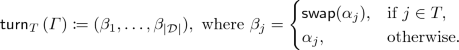
  Here, $\mathsf {swap}(\frac{c}{\mathord {?}}) := \frac{\mathord {?}}{c}$ and $\mathsf {swap}(\frac{\mathord {?}}{c}) := \frac{c}{\mathord {?}}$, for $c \in \mathcal {D}$.

• $(\mathsf {perm}, \pi )$ for a permutation $\pi \in S_{{|}{\mathcal {D}}{|}}$ from the symmetric group $S_{{|}{\mathcal {D}}{|}}$. This applies $\pi$ to the sequence, i.e., if $\varGamma =(\alpha _1, \ldots , \alpha _{{|}{\mathcal {D}}{|}})$, the resulting sequence is

  $$\begin{aligned} {\mathsf {perm}}_{\pi }\left( \varGamma \right) := (\alpha _{\pi ^{-1}(1)}, \ldots , \alpha _{\pi ^{-1}({|}{\mathcal {D}}{|})}). \end{aligned}$$

• $(\mathsf {shuffle}, \varPi , \mathcal {F})$ for a probability distribution $\mathcal {F}$ on $S_{{|}{\mathcal {D}}{|}}$ with support $\varPi$. This transforms a sequence $\varGamma$ into

  $$\begin{aligned} {\mathsf {shuffle}}_{\varPi , \mathcal {F}}\left( \varGamma \right) := {\mathsf {perm}}_{\pi }\left( \varGamma \right) , \text { for } \pi \text { drawn from }\mathcal {F}, \end{aligned}$$

  i.e., $\pi \in \varPi$ is drawn according to $\mathcal {F}$ and then applied to $\varGamma$. This is done in such a way that no player/bystander can observe anything about $\pi$ in the process. If $\mathcal {F}$ is the uniform distribution on $\varPi$, we just write $(\mathsf {shuffle}, \varPi )$.

• $(\mathsf {restart})$. This transforms a sequence into the start sequence. In that case the first component of $A$’s output must be $q_0$. This allows for Las Vegas protocols to start over and cannot be used in finite-runtime protocols.

• $(\mathsf {result}, p_1, \ldots , p_{r})$ declares the ordered sequence of cards in distinct positions $p_1, \ldots , p_{r} \in \{1, \ldots , {|}{\mathcal {D}}{|}\}$ as the output of the protocol and halts. This special operation occurs if and only if the first component of $A$’s output is $q_ f$.

A sequence trace of a finite protocol run is a tuple $(\varGamma _0, \varGamma _1, \ldots , \varGamma _t)$ of sequences such that $\varGamma _0 \in U$ and $\varGamma _{i+1}$ arises from $\varGamma _i$ by an operation as specified by the action function. Moreover, $(\mathsf {top}(\varGamma _0), \mathsf {top}(\varGamma _1), \ldots , \mathsf {top}(\varGamma _t))$ is a corresponding visible sequence trace.

Security of card-based protocols intuitively means that input and output are perfectly hidden, i.e., from the outside the execution of a protocol looks the same (has the same distribution), regardless of what input and output are.

Definition 1

(Security, cf. [KWH15, KW17]). Let $\mathcal {P} = (\mathcal {D},U,Q,A)$ be a protocol. It is (input- and output-)secure if for any random variable I with values in the set of input sequences U, the following holds. A random protocol run starting with $\varGamma _0 = I$, terminates almost surely. Moreover, if V and O are random variables denoting the visible sequence trace and the output of the run, then the pair (I, O) is stochastically independent of V.

3 State Trees and Their Properties

The authors of [KWH15] introduce a representation of secure protocols as a tree-like diagram, we call it a state tree. In it, all protocol runs are captured simultaneously in a way that makes output behavior and security of the protocol directly recognizable.

An assumption that significantly reduces notational complexity is that cards are essentially always face-down. This relates to all input and output sequences², but moreover, turn actions occur in pairs, such that cards that are turned face-up by the first turn are directly turned face-down again afterwards. After revealing the symbols, there is no reason to keep the cards face-up any longer. Corollary 2 of Sect. 4 is a formal version of this argument.

3.1 Constructing State Trees from Protocols

We describe how to construct state trees from protocol descriptions. See Fig. 1 for a reference. In the following v is always the visible sequence trace of the prefix of a protocol run.³ For each such v, the state tree contains a state $\mu _v$. In our model, each state is associated with a unique action that the protocol prescribes for this situation. We annotate the state (essentially its outgoing edge) with this action. If the action may extend v to $v'$ by appending a visible sequence $v^+$, then $\mu _{v'}$ is a child of its parent $\mu _v$. A turn action may result in several children which are siblings of each other and the edge to each child is additionally annotated with $v^+$. If the action is a result action, then $\mu _v$ is a leaf.

Fig. 1.

The six-card AND protocol of [MS09].

From the perspective of an observer of the protocol who does not know the input I or the permutations chosen during shuffle actions, the actual sequence $S_v$ lying on the table in a particular run when the state $\mu _v$ is reached, is unknown. We annotate $\mu _v$ with the corresponding probabilities, i.e. with $\mu _v(s) := \Pr [S_v = s \mid v]$ where s is any sequence of symbols and v stands for the event that v is a prefix of the visible sequence trace of the complete protocol run. We can rewrite this as:

$$\begin{aligned} \mu _v(s)&= \sum _{\varGamma \in U} \Pr [S_v = s, I = \varGamma \mid v] = \sum _{\varGamma \in U} \Pr [S_v = s \mid I = \varGamma , v]\cdot \Pr [I = \varGamma \mid v]\\&= \sum _{\varGamma \in U} \underbrace{\Pr [S_v = s \mid I = \varGamma , v]}_{=: p_{v,\varGamma ,s}}\cdot \underbrace{\Pr [I = \varGamma ]}_{=: X_\varGamma } = \sum _{\varGamma \in U} p_{v,\varGamma ,s} X_\varGamma . \end{aligned}$$

At the line-break, we exploited the independence of visible sequence trace and input in secure protocols and introduced two abbreviations. Note that $p_{v,\varGamma ,s}$ is constant, but $X_\varGamma$ is a variable since we have not actually defined a specific probability distribution on the inputs (nor will we). We treat the result as a formal sum, making $\mu _v$ a map from sequences of symbols to polynomials.

We say a state $\mu _v$ contains a sequence of symbols s (or s is in $\mu _v$ for short) if $\mu _v(s)$ is not the zero polynomial, and write $\mathrm {supp}(\mu _v)$ (as in support) for the set of all such sequences. Let $|\mu | := |\mathrm {supp}(\mu _v)|$. We now describe how the tree of all states can be computed for a given secure protocol inductively starting from the root.

Start state. First note that the start state is unique: Regardless of the (face-down) input sequence, the visible sequence trace is $v_0 = \left( (?,\ldots ,?)\right)$ only containing one trivial visible sequence. The distribution of $S_{v_0}$ is the input distribution, i.e.,

$$ \mu _{v_0}(s) = {\left\{ \begin{array}{ll} X_\varGamma , &{} \text { if } s = \mathsf {symb}(\varGamma ) \text { for } \varGamma \in U,\\ 0, &{} \text { otherwise. } \end{array}\right. } $$

Shuffle action. Assume for a state $\mu _v$ the action $(\mathsf {shuffle}, \varPi , \mathcal {F})$ is prescribed. No non-trivial information is revealed when shuffling, so obtaining $v'$ by appending a trivial visible sequence to v, $\mu _{v'}$ is the unique child of $\mu _v$, fulfilling

$$\begin{aligned} \mu _{v'}(s')&= \Pr [S_{v'} = s' \mid v'] \\&= \sum _{\pi \in \varPi } \mathcal {F}(\pi ) \cdot \Pr [S_v = \pi ^{-1}(s') \mid v] = \sum _{\pi \in \varPi } \mathcal {F}(\pi ) \cdot \mu _v(\pi ^{-1}(s')). \end{aligned}$$

This just takes into account all sequences $\pi ^{-1}(s')$ in $\mu$ from which $s'$ may have originated from via some $\pi$ as well as corresponding probabilities.

Note that perm actions are a special case and need not be described separately.

Restart action. States in which a restart action happens have a single child. The subtree at this child is equal to the entire tree.

Turn action. Let $\mu _v$ be a state with a turn action that possibly results in the visible sequence $v^+$, which appended to v yields $v'$. The child $\mu _{v'}$ of $\mu _v$ contains those sequences from $\mu _v$ that are compatible with $v^+$, i.e., equal to $v^+$ in the positions i with $v^+[i] \ne {?}$. Moreover, the probability to reach $\mu _{v'}$ from $\mu _v$ is:

Recall that the right hand side is a polynomial of the form $\sum _{\varGamma \in U} a_{\varGamma } X_{\varGamma }$ where $X_{\varGamma }$ is a placeholder for the input probability $\Pr [I = \varGamma ]$. By security, input and visible sequence trace are independent, in particular no matter how the variables $(X_{\varGamma })_{\varGamma \in U}$ are initialized, the polynomial $\Pr [v' \mid v]$ evaluates to the same real number. Thus, all $a_{\varGamma }$ are equal to a constant $\lambda _{v'} \in [0,1]$ and using $\sum _{\varGamma \in U} X_{\varGamma } = 1$ we have:

Moreover, for $s \in \mathrm {supp}(\mu _{v'})$ we have:

$$\begin{aligned} \mu _{v'}(s) = \Pr [S_{v'} = s \mid v'] = \frac{\Pr [S_{v'} = s \mid v]}{\Pr [v' \mid v]} = \frac{\Pr [S_v = s \mid v]}{\lambda _{v'}} = \frac{\mu _v(s)}{\lambda _{v'}}. \end{aligned}$$

Hence, $\mu _{v'}$ is a restriction of $\mu _v$ to sequences compatible with $v'$, scaled by $\frac{1}{\lambda _{v'}}$. Capturing the observation we made for secure protocols, we define

(1)

Output behavior. Consider any leaf state $\mu _v$ with action $(\mathsf {result},p_1,p_2,\ldots ,p_r)$. The output $O = (S_v)_{p_1,\ldots ,p_r}$ is the projection of $S_v$ to the components $p_1,\ldots ,p_r$. We can easily obtain from $\mu _v$ the probabilities $\Pr [O = o \mid v]$ for any sequence of symbols o. By security, the visible sequence trace v is irrelevant, which implies that we obtain the same polynomial $\Pr [O = o]$ for a fixed o, regardless of which leaf state we examine. If the protocol computes a deterministic function (see below), this polynomial is the sum of all $X_\varGamma$ for which $\varGamma$ evaluates to o.

3.2 The Utility of State Trees

In the following proposition we argue that state trees are a superior way to represent secure protocols, as security and correctness are more tangible.

Proposition 1

Every secure protocol $\mathcal {P}$ has a unique state tree that can be obtained as described above. Moreover, local checks suffice to verify that a tree of states describes a secure protocol with a desired output behavior.

Proof

The proof is given in the full version. By local checks we mean checking that each state arises from its parent in the way we discussed. In particular, for turns, the probability of sequences compatible with an outcome must sum to a constant and all leaf states must provide the same output distribution.   $\square$

State trees can be infinite while state machines are typically required to have a finite number of states. This is mostly beside the point for our purposes, but the claim should be understood with the following qualification. Either a countably infinite number of states is permitted for protocols or only certain self-similar state trees can be transformed into protocols (see Fig. 3 for such a state tree).

Runtime of a Protocol. A secure protocol terminates when entering the final state $q_ f$. It has finite-runtime, if there is an a priori upper bound on the number of steps. It is Las Vegas if it terminates almost surely in a number of steps that is finite in expectation, but unbounded.

We restate these definitions with respect to state trees. A path in a state tree p starts at the root and descends according to a visible sequence trace v. If v is finite, p ends in a leaf. The probability of p is $\Pr [v]$, which is a constant (independent of the distribution of inputs) by our discussion of security before. We say that a protocol is finite-runtime if there is no infinite path in its state tree. If a protocol is not finite-runtime but the expected length of any path in its state tree is finite, we call it a Las Vegas protocol.

3.3 Protocols Computing a Boolean Function

The way we defined it, a protocol takes an unstructured input and computes an unstructured output that is in general a randomized function of the input. While randomization (as in privately computing a fixed-point-free permutation [CK93]) and unstructured (non-committed) outputs (as in the “five card trick” [dBoe89]) appear in the literature, the most important use case is arguably the computation of a deterministic Boolean function in committed format. In this section we provide useful terminology and some simple insights for this setting.

The Setting. A commitment to a bit value $b \in \{0,1\}$ is represented by two cards, with their symbols arranged as $\heartsuit \,\clubsuit$ if $b=1$ and as $\clubsuit \,\heartsuit$ otherwise. Extend this in the natural way, we say a sequence of symbols (or cards) $(\alpha _1,\ldots ,\alpha _{2k})$ encodes a sequence $b \in \{0,1\}^k$ of bits, if $\alpha _{2i-1} \alpha _{2i}$ (or $\mathsf {top}(\alpha _{2i-1}) \mathsf {top}(\alpha _{2i})$) represents b[i] for $1 \le i \le k$. We say that a protocol $\mathcal {P} = (\mathcal {D}, U, Q, A)$ computes a function $f:\{0,1\}^k \rightarrow \{0,1\}^\ell$, if the following holds:

• The deck $\mathcal {D}$ contains at least $\max (k, \ell )$ cards of each symbol,

• There is an input sequence $\varGamma _b$ for each $b \in \{0,1\}^k$, the first 2k cards of which encode b. The remaining ${|}{\mathcal {D}}{|}- 2k$ cards are independent of $b$. Favoring light notation, we use b instead of $\varGamma _b$ as index to refer to variables from the family $(X_b)_{b \in \{0,1\}^k} = (X_\varGamma )_{\varGamma \in U}$ from now on.

• Correctness: A protocol run starting with $\varGamma _b$ almost surely terminates with an output encoding f(b).

We call a protocol computing $f_{\wedge }:\{0,1\}^2 \rightarrow \{0,1\}$, with $(a,b) \mapsto a \wedge b$ an AND protocol. A protocols computing $f_{\text {copy}}:\{0,1\} \rightarrow \{0,1\}^n$, with $a \mapsto a^n = (a, \ldots , a)$ and $n \ge 2$ is called an $n$-COPY or just COPY protocol.

Figures 1, 2 and 3 depict state trees of current AND and COPY protocols, which are identified as card-minimal with respect to certain restrictions, in this paper. See the full version for a discussion of the security and correctness of Fig. 1.

Fig. 2.

The state tree of the $(2n+2)$-card COPY protocol [MS09]. As in the six-card AND protocol, the shuffle consists only of the identity and a permutation that is a cycle decomposition into (disjoint) $2$-cycles. Hence, it can be implemented by a random bisection cut. See [CHL13, Sect. 6] for a more elaborate explanation.

Fig. 3.

A variant of the $(2n+1)$-card COPY protocol of Nishimura et al. [NNH+17, Sect. 5], with less permuting. After the permutation in the first $\heartsuit$-branch, the protocol resembles a $2$-COPY protocol [NNH+15] on the first four and the last card. The parentheses $(\cdot )^1$ are to emphasize this symmetry. The shuffle steps in this protocol are uniform, but non-closed. As they consist of the identity and exactly one odd-length cycle, they can be performed using an “unequal division shuffle”. A proposed implementation of these shuffles using sliding cover boxes or envelopes can be found in [NNH+17, Sect. 6]. Although this diagram includes a backwards edge, this is for presentation only. We regard it as an infinite (self-similar) tree.

3.4 Reduced State Trees and Possibilistic Security

When trying to prove that no secure protocol with certain properties exists, the space of possible states can seem vast. We therefore opt to show stronger results, namely the non-existence of protocols with the weakened requirement of possibilistic security, defined next. This allows to consider a projection of the state space which is finite in size.

Definition 2

A protocol $\mathcal {P}=(\mathcal {D}, U, Q, A)$ computing a function $f:\{0,1\}^k \rightarrow \{0,1\}^{\ell }$ has possibilistic input security (possibilistic output security) if it is correct, i.e., $O = f(I)$ almost surely and for uniformly⁴ random input $I \in U$ and any visible sequence trace v with $\Pr [v] > 0$ as well as any input $i \in \{0,1\}^k$ (any output $o \in \{0,1\}^{\ell }$) we have $\Pr [v \mid I = i] > 0$ ($\Pr [v \mid f(I) = o]$).

In other words, from observing a visible sequence trace it is never possible to exclude an input (or output) with certainty. Clearly, security implies possibilistic input and output security. To decide whether a protocol has possibilistic output security, it suffices to consider projections of states in the following sense.

Definition 3

(adapted from [KWH15]). Let $\mathcal {P}=(\mathcal {D}, U, Q, A)$ be a protocol computing a function $f:\{0,1\}^k \rightarrow \{0,1\}^{\ell }$. If $\mu$ is a state in the state tree, then the reduced state $\hat{\mu }$ has the same sequences as $\mu$ with simpler annotations. Assume $\mu (s)$ is a polynomial with positive coefficients for the variables $X_{b_1},\ldots ,X_{b_i}$ ($i \ge 1$). Then we set $\hat{\mu }(s) = o \in \{0,1\}^{\ell }$ if $o = f(b_1) = f(b_2) = \ldots = f(b_i)$. If not all $b_i$ evaluate to the same output under f, set $\hat{\mu }(s) = \bot$. Accordingly, sequences in $\hat{\mu }$ are called o-sequences or $\perp$-sequences. We also say they are of type o or of type $\bot$, respectively. For COPY protocols, we call $1^\ell$- and $0^\ell$-sequences just $1$- and $0$-sequences, respectively.

Note that if a state $\mu$ has children $\mu _1,\ldots ,\mu _i$ in the state tree, then the reduced states $\hat{\mu }_1, \ldots , \hat{\mu }_i$ can be computed from the reduced state $\hat{\mu }$. In particular, it makes sense to define reduced state trees as projections of state trees and aim to prove the non-existence of certain state trees by proving the non-existence of the corresponding reduced state trees.

3.5 Important Properties of (Reduced) States

For most of our arguments, reduced states offer a sufficient granularity of detail and the following observations and definitions for reduced states will prove useful. Clearly, they also apply to the richer, non-reduced states which we will briefly require for a more subtle argument in Sect. 7.

Protocols computing a function f that have a $\perp$-sequence in a reduced state cannot be restart-free, and hence also not finite-runtime: once the $\perp$-sequence is actually on the table, it does not contain sufficient information to deduce the unique correct output, making a restart necessary. The protocol might then repeat the unfortunate path of execution an arbitrary number of times.

We call two reduced states similar, if one is just a permuted version of the other, i.e. interpreting a state as a matrix of symbols with annotated rows, there is a permutation on the columns mapping one state to the other.

In restart-free protocols with two outputs (say 1 and 0) any reduced state $\hat{\mu }$ is composed of some number i of 0-sequences and some number j of 1-sequences with $|\hat{\mu }| = i + j$. We call $\mu$ and $\hat{\mu }$ an i / j-state. They are final if they admit a correct output action $(\mathsf {result},m_1,n_1\ldots , m_\ell , n_\ell )$, i.e. they does not contain a $\bot$-sequence and for all outputs $r \in \{0,1\}^\ell$ there is at least one $r$-sequence and $r$-sequences have a $\heartsuit$ at position $m_i$ if $r[i]=1$, or a $\clubsuit$ otherwise, for all $1\le i\le \ell$, and the respective other symbol at position $n_i$.

Turnable Positions. Recall the definition of a turnable position for a state $\mu$ from (1). For a reduced state $\hat{\mu }$ this simplifies to: For each symbol c occurring in column i, among the sequences with $s[i] = c$, there is either a $\perp$-sequence or an r-sequence for each $r \in \{0,1\}^\ell$. If some position in a (reduced) state is turnable, we call the state turnable, otherwise unturnable.

4 Simplifications to the Computational Model

In the following, we argue that public randomness does not provide any benefit in secure protocols and hence can be safely excluded from the computational model. For this assume there was an additional class of actions in protocols, that produces public randomness: The action $\mathsf {rand}(p_1,\ldots ,p_i)$ for real numbers $p_1,\ldots ,p_i \in (0,1)$ summing to 1 appends a value $x \in \{0,1,\ldots ,i\}$ to the visible sequence trace with $\Pr [x = j] = p_j$. This extends the computational model⁵. An example would be a protocol that receives a bit in committed format, and outputs either this bit unchanged with probability or its negation with probability . This can be implemented by a action and, depending on the outcome a permutation or not, followed by a result action. This is also possible with a shuffle, but requires a non-uniform probability distribution on the permutations, something we are inclined to prohibit later. However, this protocol is not secure since the result of the random experiment is part of the visible sequence trace (it is public) which introduces a non-trivial relationship between output and visible sequence trace precluding independence. Indeed we show:

Proposition 2

(Public randomness is unnecessary). Any $\mathsf {rand}(p_1,\ldots ,p_i)$ action can be removed from a secure protocol $\mathcal {P}$ without affecting security or the output distribution and without increasing (worst-case or expected) runtime.

Proof

Consider i copies $\mathcal {P}_1,\ldots ,\mathcal {P}_i$ of $\mathcal {P}$, where in $\mathcal {P}_j$, if the $\mathsf {rand}$ action is encountered, execution continues deterministically as if j had been chosen. The distribution of input output and visible sequence trace $(I_j,O_j,V_j)$ for $\mathcal {P}_j$ equals the distribution of (I, O, V) for $\mathcal {P}$, except conditioned under a certain event $E_j$ regarding V. In particular, independence of (I, O) and V implies independences of $(I_j,O_j)$ and $V_j$ and $(I_j,O_j)$ is distributed like (I, O) (security and output behavior are unaffected). Thus, choosing j such that $V_j$ has least (worst-case or expected) length gives the desired modification $\mathcal {P}_j$ of $\mathcal {P}$.    $\square$

Mizuki and Shizuya [MS14] introduced a randomized action called $\mathsf {rflip}$ that works just like a turn-action, except the set of cards T that is turned is chosen randomly according to some distribution. We call it randomized flip. As the random choice is clearly public we can directly derive the following:

Corollary 1

The randomized flip can be removed from a secure protocol without negative effects as in Proposition 2.

When introducing state trees, we assumed that cards are always face-down, in particular during shuffle operations. This hides a complication: Shuffling with face-up cards, i.e., with the current visible sequence v being non-trivial, may result in several visible sequences $v'$, depending on how the face-up cards are permuted. But similar to rflip, such a branching shuffle can be simulated with a $\mathsf {rand}$ action, determining which $v'$ is obtained, followed by a shuffle action restricted to those permutations that transform v into $v'$. From the discussion above, we can derive the following corollary.

Corollary 2

(We can assume all cards are face down). It suffices to look at protocols which start with face-down cards and which, after turning any card, directly turns them down again.

In Lemma 4 we argue that this still works for uniform and/or closed shuffles, i.e. if the original branching shuffle was closed (uniform), the restricted shuffles can be implemented using closed (uniform) shuffles as well.

5 Properties of Restricted-Shuffle Protocols

As discussed before, it is natural to restrict card-based protocols to closed shuffles. The fact that a closed permutation set $\varPi$ is a subgroup of the symmetric group $S_{{|}{\mathcal {D}}{|}}$ implies strong structural properties for the corresponding shuffle action on states. This structure is captured by the orbits associated with the group action of $\varPi$ on sequences on symbols, introduced in the following.

Definition 4

(Group action, e.g. [DM96]). Let X be a nonempty set, G a group, and $\varphi :G \times X \rightarrow X$ a function written as $g(x) := \varphi (g,x)$ for $g \in G, x \in X$. We say that G acts on X if

• $e(x) = x$ for all $x \in X$, where e denotes the identity element in G,

• $(g \circ h) (x) = g (h(x))$ for all $x \in X$ and all $g,h \in G$.

In card-based protocols, the permutation group $S_{|\mathcal {D}|}$ acts on a set of sequences of a deck $\mathcal {D}$ in the natural way, by reordering the cards in a sequence according to the permutation.

For a group G acting on a set X the orbit of an element $x \in X$ is $G(x) = \{g(x):g \in G\}$. Any subgroup of $S_{|\mathcal {D}|}$ also acts on X in the same way. This is interesting for closed shuffle operations. The orbit of an element $x$ under a subgroup $\varPi$ is $\varPi (x) = \{\pi (x):\pi \in \varPi \}$. It is easy to see that the orbits of two elements are either the same or disjoint. Therefore, $\varPi$ induces a partition of the set of possible sequences into disjoint orbits. We call this partition the orbit partition of the sequences through $\varPi$. For a shuffle with permutation set $\varPi$ we also say that the orbit partition of $\varPi$ is the orbit partition of the shuffle.

5.1 Properties of (Uniform) Closed Shuffles

For our proof we will need the orbit partitions of closed shuffles on sequences of five cards with three $\heartsuit$ and two $\clubsuit$. A display of all relevant orbit partitions can be seen in Fig. 4. Before we proceed with the main theorem in Sect. 7, it is beneficial to state some observations about orbit partitions and closed shuffles.

Fig. 4.

Orbits of different closed (cyclic) shuffle operations on the card sequences.

Lemma 1

Assume we shuffle a state $\mu$ into a state $\mu '$ using a closed permutation set $\varPi$. If there is $\pi \in \varPi$ with $\pi (i) = j$, then in $\mu '$ the columns i and j contain the same multiset of symbols.

Proof

Assume column i has k $\clubsuit$ in $\mu '$. Because $\varPi$ is closed, shuffling again with $\varPi$ yields $\mu '$ again. In particular if $s'$ is contained in $\mu '$, then so is $\pi (s')$. Since $\pi$ is a bijection on the set of all sequences, the sequences with $\clubsuit$ in position i are mapped to distinct sequences with $\clubsuit$ in position j. In particular column j contains at least as many $\clubsuit$ as column i in $\mu '$. Since the same argument works for all other symbols and the total number of sequences did not increase, the numbers of $\clubsuit$ (and other symbols) in column i and j coincides. Since $\clubsuit$ was arbitrary, the claim follows.   $\square$

Observe that Lemma 1 is false, if $\varPi$ is not closed. Take for instance an action $(\mathsf {perm},\pi )$ for $\pi \ne {\mathsf {id}}$. It is a non-closed shuffle clearly lacking this property.

Lemma 2

(Shuffling and Orbit Partitions). Let $\mu$ be transformed into $\mu '$ via some shuffle with closed permutation set $\varPi$. Let $O$ be an orbit of $\varPi$.

• 1. If $\mu \cap O = \emptyset$, then⁶ $\mu '\cap O = \emptyset$

• 2. If $\mu \cap O$ contains a sequence of type $r$ and no other sequences of type $r'\ne r$, then $\mu '\cap O = O$ contains only $r$-sequences.

• 3. Otherwise, $\mu '\cap O = O$ contains only $\bot$-sequences.

Proof

Note that for any pair $s_1,s_2$ of sequences, there is some $\pi \in \varPi$ with $\pi (s_1) = s_2$ precisely if they are in the same orbit of $\varPi$. Thus when shuffling with $\varPi$, the type $\mu (s_1)$ directly “infects” precisely the entire orbit of $s_1$. With $\perp$ indicating several types jumbled together, the three cases are easily checked.    $\square$

For the more restricted case of uniform closed shuffles, let us state the following simple but interesting observation: all sequences in an orbit have the same symbolic probability after the shuffle.

Lemma 3

Let $\mathsf {act} = (\mathsf {shuffle}, \varPi )$ be a uniform closed shuffle and $\mu$ a state. Let $\mu '$ be the state arising from $\mu$ through $\mathsf {act}$ and $s_1'$ and $s_2'$ two sequences of symbols in $\mu '$. If $s_1' = \pi (s_2')$ for $\pi \in \varPi$, then $\mu '(s_1') = \mu '(s_2')$, i.e., the sequences have the same probability.

Finally, let us note that it is not possible to perform shuffles that are more powerful than closed shuffles indirectly by using a closed shuffle while cards are face-up (branching shuffles). This re-vindicates an assumption made in Sect. 4. Taking into account Corollary 2, we need only prove the following:

Lemma 4

Let $\varPi$ be any closed permutation set and v and $v'$ visible sequences. Assume $\varPi _{v \rightarrow v'} := \{ \pi \in \varPi :\pi (v) = v'\}$ is non-empty. Then for any $\pi _{v \rightarrow v'} \in \varPi _{v \rightarrow v'}$, the set $\varPi _v := \varPi _{v \rightarrow v'} \circ \pi _{v \rightarrow v'}^{-1}$ is closed.

In particular, we can implement $(\mathsf {shuffle}, \varPi _{v \rightarrow v'})$ using $(\mathsf {perm}, \pi _{v \rightarrow v'})$ followed by the closed shuffle $(\mathsf {shuffle}, \varPi _{v})$.

Proof

Let $x = \varphi _1 \circ \pi _{v \rightarrow v'}^{-1}$ and $y = \varphi _2 \circ \pi _{v \rightarrow v'}^{-1}$ be two elements of $\varPi _v$, in particular $\varphi _1,\varphi _2 \in \varPi _{v \rightarrow v'}$. We have $(\varphi _1 \circ \pi _{v \rightarrow v'}^{-1} \circ \varphi _2)(v) = v'$, so $\varphi _1 \circ \pi _{v \rightarrow v'}^{-1} \circ \varphi _2 \in \varPi _{v \rightarrow v'}$. This implies:

$$x \circ y = \varphi _1 \circ \pi _{v \rightarrow v'}^{-1} \circ \varphi _2 \circ \pi _{v \rightarrow v'}^{-1} \in \varPi _{v \rightarrow v'} \circ \pi _{v \rightarrow v'}^{-1} = \varPi _v.$$

   $\square$

For uniform shuffles, the analogous claim is even easier, as a uniformly random variable conditioned to be contained in some subset is still uniform on that subset. For uniform and closed shuffles these arguments can be combined.

6 Impossibility of Five-Card Finite-Runtime AND Protocols with Closed Shuffles

In this section, we prove that AND protocols which are restricted to closed shuffle operations, require six cards. The proof uses a similar technique as in [KWH15, Sect. 6]. While in the latter there was a set of good states including the final states which you never enter with all branches of a branching point in the protocol, here we found that it was easier to start the other way round, namely to define a set of bad states, about which we prove that starting from these there is always a path in the tree which will enter a bad state again and this path does not contain any final states. Here the situation is more complex as there are many more possible states and we needed to derive new tools (orbit partitions) to make use of the structure of the restricted permutation sets. For this we will make heavy use of Lemmas 1 and 2, because they enable us to exploit the rich structure of closed shuffles. Let us begin by stating our theorem.

Theorem 1

Let $\mathcal {P}$ be a (possibilistically) secure protocol computing AND in committed format using only closed shuffles with five cards of two symbols.⁷ Then $\mathcal {P}$ is not finite-runtime.

Proof Outline. We define a set of bad states, such that the start state is one of them. We then show that in any protocol from each bad state there is a path into another bad state. In particular, none of the bad states and none of the states on the paths between them are final. This implies that there is an infinite path starting from the start state precluding finite runtime.

Without loss of generality, the protocols we consider have the following properties, since each protocol that does not have some of these properties can be transformed into an equivalent protocol that does.

• $\mathcal {P}$ does not use operations that transform a (reduced) state into any similar state. These operations are clearly not necessary, when arguing about possibilistic security, which is sufficient in our case.

• $\mathcal {P}$ does not use shuffle operations while cards are lying face up. These are unnecessary by Corollary 2 and Lemma 4.

• each shuffle set $\varPi$ is a cyclic subgroup of $S_5$. This is because each subgroup $\varPi$ of $S_5$ can be written as the product $\varPi = \prod _{\pi \in \varPi } {\langle }{\pi }{\rangle }$, implying that doing the cyclic shuffles ${\langle }{\pi }{\rangle }$ one after the other gives the same set of permutations that can happen in total as in $\varPi$ itself.

• The deck is $\mathcal {D}= {[}{\heartsuit ,\heartsuit ,\heartsuit ,\clubsuit ,\clubsuit }{]}$. We need two $\clubsuit$ and two $\heartsuit$ for the inputs. Our arguments work regardless of whether the fifth card is $\clubsuit$ or $\heartsuit$.

Definition of Bad States. Any state $\mu$ with one of the following properties is bad:

$\mathcal {B}_{4*}$::

$\mu$ has four sequences of the same type. In particular, this includes all states with seven or more sequences,

$\mathcal {B}_{3\clubsuit }$::

$\mu$ has a constant $\clubsuit$-column and three or more sequences,

$\mathcal {B}_{5\heartsuit }$::

$\mu$ has a constant $\heartsuit$-column and five or more sequences,

$\mathcal {B}_{3\heartsuit \heartsuit }$::

$\mu$ has two constant $\heartsuit$-columns and three sequences,

$\mathcal {B}_{\heartsuit 3/1}$::

$\mu$ has a constant $\heartsuit$-column and is of type 3/1 or 1/3.

To see that states of these types are all non-final, first note that any final state is, up to reordering, a (not necessarily proper) subset of the sequences of the following state including at least one 0-sequence and at least one 1-sequence. Hence, we will call it the maximal final state:

The bad states do not “fit” into this state, since

$\mathcal {B}_{4*}$::

the maximal final state has only three sequences of each type.

$\mathcal {B}_{3\clubsuit }$::

the only two columns in the maximal final state with three $\clubsuit$ are the first two. But a restriction to the sequences with $\clubsuit$ in the first (or second) position contains 0-sequences (1-sequences) only.

$\mathcal {B}_{5\heartsuit }$::

all columns of the maximal final state contain at most four $\heartsuit$.

$\mathcal {B}_{3\heartsuit \heartsuit }$::

no two columns in the maximal final state have three $\heartsuit$ in the same positions.

$\mathcal {B}_{\heartsuit 3/1}$::

any admissible restriction of the maximal final state with four sequences and a constant $\heartsuit$-column is of type 2/2.

The start state is bad as required as it falls into category $\mathcal {B}_{\heartsuit 3/1}$. We begin by making a few observations that greatly simplify the proof.

Claim

(Restriction to Simple Shuffles). We need to only consider the three shuffle sets ${\langle }{(1\,2)}{\rangle }, {\langle }{(1\,2\,3)}{\rangle }$ and ${\langle }{(1\,2)(3\,4)}{\rangle }$ in the main proof.

Proof

As discussed before, we only consider cyclic shuffles, i.e. shuffles of the form $\varPi = {\langle }{\pi }{\rangle }$ for $\pi \in S_{{|}{\mathcal {D}}{|}}$. Unless $\pi = {\mathsf {id}}$, the cycle decomposition of $\pi$ can have either one cycle of length 2, 3, 4 or 5 or two cycles of length 2 or one cycle of length 2 and one cycle of length 3. We treat states that are equal up to similarity (reordering) as equivalent; it therefore suffices to consider one shuffle of each type. Among them, ${\langle }{(1\;2)(3\;4\;5)}{\rangle }$ can be decomposed⁸ as ${\langle }{(1\;2)}{\rangle }\circ {\langle }{(3\;4\;5)}{\rangle }$ and we handle those factors anyway. In the cases ${\langle }{(1\;2\;3\;4\;5)}{\rangle }$ and ${\langle }{(1\;2\;3\;4)}{\rangle }$ there is no choice of two orbits such that both contain less than four sequences, so any shuffle that does not produce $\perp$-sequences will produce at least four sequences of the same type, yielding a bad state of type $\mathcal {B}_{4*}$.   $\square$

Claim

(Criteria for Dead Columns). The following criteria for columns ensure that if the next turn in the protocol occurs in this column, then we are either already bad or this turn entails a bad successor state. We say the column is dead.⁹ In particular, if all columns are dead, we know that after the next turn, we get a bad state.

$\mathcal {D}_{3\clubsuit }$::

The column contains 3 $\clubsuit$.

$\mathcal {D}_{5\heartsuit }$::

The column contains 5 $\heartsuit$.

$\mathcal {D}_{2*\clubsuit }$::

The column contains 2 $\clubsuit$ belonging to sequences of the same type.

$\mathcal {D}_{3*\heartsuit }$::

The column contains 3 $\heartsuit$ belonging to sequences of the same type.

Proof

• If a column contains three or more $\clubsuit$, turning this column yields a bad state with a constant $\clubsuit$-column and three or more sequences.

• If a column contains five or more $\heartsuit$, turning this column yields a bad state with a constant $\heartsuit$-column and five or more sequences.

• if a column contains two $\clubsuit$ belonging to sequences of the same type, an additional sequence of the other type with $\clubsuit$ must be added in this position to make it turnable. This leads to a column with three $\clubsuit$, and turning there yields a $\mathcal {B}_{3\clubsuit }$.

• If three sequences of the same type all have $\heartsuit$ in a column, there needs to be an additional sequence of this type with $\clubsuit$ in this column to make it turnable. Adding such a sequence yields a bad state of type $\mathcal {B}_{4*}$.   $\square$

Claim

(Death is Contagious). Consider a dead column with index i in a state $\mu$ and a closed shuffle $\mathsf {act}$ with permutation set $\varPi$ such that $\pi (i) = j$ for a $\pi \in \varPi$. Then the column with index j is dead as well after applying $\mathsf {act}$ to $\mu$.

Proof

• By Lemma 1, the number of $\clubsuit$ must be the same in columns i and j after the shuffle. Therefore $\mathcal {D}_{3\clubsuit }$ spreads.

• This case is completely analogous to the previous, with $\mathcal {D}_{5\heartsuit }$ instead of $\mathcal {D}_{3\clubsuit }$.

• By Lemma 1 column j must have at least two $\clubsuit$ in the same type of sequences after the shuffle.

• For any shuffle that does not create $\bot$-sequences, by Lemma 1 there must be three sequences of the same type that have $\heartsuit$ in column j. Therefore j is dead after the shuffle.   $\square$

Proof

(of Theorem  1). We show that from each bad state there is a path into another bad state by case analysis.

• States with four sequences of the same type. Any non-trivial shuffle not producing $\bot$-sequences retains the four sequences of the same type.

  Assume w.l.o.g. that there are four 0-sequences and consider turn operations. This requires at least two 1-sequences. If there are two sequences of type 1, we have six sequences in total. Turning either yields two states of at least three sequences, in particular one with constant $\clubsuit$, a $\mathcal {B}_{3\clubsuit }$, or a 3/1 state with constant $\heartsuit$, a $\mathcal {B}_{\heartsuit 3/1}$. If there are more that two $1$-sequences, there are at least seven sequences in total. A turn yields two successor states – one with a constant $\heartsuit$-column and k sequences, and one with a constant $\clubsuit$-column with $\ell$ sequences and $k + \ell \ge 7$. So we have $k \ge 5$ ($\mathcal {B}_{5\heartsuit }$) or $\ell \ge 3$ ($\mathcal {B}_{3\clubsuit }$).

• States with a constant $\clubsuit$-column and four sequences. Up to reordering, the state looks like

  

  This state admits no non-trivial turn operation. Any shuffle operation that does not involve the first column produces a similar state. Since any column other than the first contains three $\heartsuit$, any other shuffle produces three additional $\heartsuit$ in the first column by Lemma 1, resulting in a state of type $\mathcal {B}_{4*}$.

• States with a constant $\clubsuit$-column and three sequences. Without loss of generality, these states are of type 2/1. They are non-turnable. Shuffles that do not involve the constant column will retain the property of being constant $\clubsuit$ in that column and three or more sequences. Hence, in the following we consider shuffles involving the constant column.

  To keep the proof simple, an important tool are the orbit partitions of each of the three equivalence classes of shuffles, as in Fig. 4. We try to place the sequences into the orbits, s.t. completing these does not yield a bad state. W.l.o.g. we choose sequences, s.t. the constant $\clubsuit$-column is the first column.

  • Case 1: $(1\,2)$. The orbit partition looks as in Fig. 4a. The first three orbits contain no $\clubsuit$ there and are out. No orbits contain two $\clubsuit$ in the first column, so both 0-sequences must be placed in distinct orbits. If both orbits are of size 2, shuffling yields four 0-sequences giving a $\mathcal {B}_{4*}$-state. Otherwise, one of the 0-sequences is $\clubsuit \clubsuit \heartsuit \heartsuit \heartsuit$. The other 0-sequence and the 1-sequence must be placed into orbits of size 2. All of them have $\clubsuit$ only in one column out of the columns 3, 4, 5, and $\clubsuit \clubsuit \heartsuit \heartsuit \heartsuit$ has $\clubsuit$ in none of them, so for all choices we end up in a $\mathcal {B}_{5\heartsuit }$-state.

  • Case 2: $(1\,2)(3\,4)$. Similarly to before, we need to choose one 0-sequence as $\clubsuit \clubsuit \heartsuit \heartsuit \heartsuit$ and need to place the remaining two sequences into the last three orbits of Fig. 4b. Choosing orbit 4 and 5 yields a $\mathcal {B}_{5\heartsuit }$-state.

    If we choose orbits 4 (or 5) and 6 then the first two columns are dead ($\mathcal {D}_{3\clubsuit }$) and the fifth column is dead as well ($\mathcal {D}_{2*\clubsuit }$). If we choose the second 0-sequence within orbit 6, then columns 3 and 4 are dead ($\mathcal {D}_{3*\heartsuit }$).

    If we choose the 0-sequence within orbit 4 (or 5) and the 1-sequence within orbit 6, there are two living non-turnable columns. Any shuffle that contains only columns 3 and 4 in one cycle does not produce a 1-sequence with $\clubsuit$ in those columns, so they remain non-turnable. Any shuffle that makes column 3 or 4 turnable by shuffling them with at least one of the dead columns kills the column in the process.

  • Case 3: $(1\,2\,3)$. If we place the three sequences in the pairwise distinct orbits of Fig. 4d, we end up with nine sequences after the shuffle. Otherwise, the two 0-sequences share the bottommost orbit and the 1-sequence must be in the second or third orbit, and we get a $\mathcal {B}_{5\heartsuit }$-state.

• States with a constant $\heartsuit$-column and five or more sequences. W.l.o.g. the first column is constant $\heartsuit$. Consider a turn operation on column $i \ne 1$. Column i has either three $\heartsuit$ and turning therefore leads to a $\mathcal {B}_{3\heartsuit \heartsuit }$-state, or column i has three $\clubsuit$ and turning leads to a $\mathcal {B}_{3\clubsuit }$-state.

  Any shuffle not involving the first column keeps it constant $\heartsuit$, and therefore bad. Consider any shuffle involving the first column, say $\pi$ is a possible permutation in the permutation set of the shuffle with $\pi (i) = 1$. Column i contains at least two $\clubsuit$ and by Lemma 1 shuffling yields two new sequences with $\clubsuit$ in position 1, giving seven or more sequences – a $\mathcal {B}_{4*}$-state.

• States with two constant $\heartsuit$-columns and three sequences. No turn operation is possible as the state is of type 1/2 or 2/1. Shuffles involving none of the constant columns keep them constant. Shuffles involving only one of them, produce a state with two $\clubsuit$ in that column, so five sequences in total, where the other $\heartsuit$-column stays constant. This is a $\mathcal {B}_{5\heartsuit }$-state.

  For the interesting case of shuffles involving both constant $\heartsuit$-columns, we again try to place the sequences into the orbits of the different types of shuffles such that completing these orbits does not yield two or more additional 0-sequences, as this would lead to a 4/2 state or to seven or more sequences.

  • Case 1: $(1\,2)$. As both constant columns have to be involved in the shuffle, they have to be in positions 1 and 2. This leaves the state constant.

  • Case 2: $(1\,2)(3\,4)$. If the constant $\heartsuit$-columns are both in the same cycle, we do not get additional sequences. Otherwise, say they are in positions 2 and 3, the only three sequences are $\heartsuit \heartsuit \heartsuit \clubsuit \clubsuit$ from orbit 2, $\clubsuit \heartsuit \heartsuit \clubsuit \heartsuit$ from orbit 5, and $\clubsuit \heartsuit \heartsuit \heartsuit \clubsuit$ from orbit 6, and shuffling results in a $\mathcal {B}_{4*}$-state.

  • Case 3: $(1\,2\,3)$. W.l.o.g. the constant columns are 1 and 2. The sequences with $\heartsuit$ in those positions are all in distinct orbits with a combined size of 7, which is a $\mathcal {B}_{4*}$-state.

• 3/1-states with a constant $\heartsuit$-column. This state is not turnable as it has only one 1-sequence. A non-trivial shuffle not involving the constant column yields a state with five or more sequences and a constant $\heartsuit$-column. For shuffles involving the constant column we try to place the sequences into the orbits of the different classes of shuffles such that completing these orbits does not yield any additional 0-sequences.

  • Case 1: $(1\,2)$. We have to involve the constant $\heartsuit$-column, which is w.l.o.g. in position 1. The only orbits with constant $\heartsuit$ are 1, 2 and 3. To not produce additional 0-sequences, those need to be the ones occupied by the 0-sequences. We need to place the 1-sequence in orbits 5, 6 or 7, and choose w.l.o.g. 5. Then, the first two columns are dead via $\mathcal {D}_{3*\heartsuit }$. The third column is dead via $\mathcal {D}_{3\clubsuit }$. Columns 4 and 5 are dead via $\mathcal {D}_{2*\clubsuit }$.

  • Case 2: $(1\,2)(3\,4)$. Regardless, the first two columns are dead via $\mathcal {D}_{3*\heartsuit }$ and the other columns are dead via $\mathcal {D}_{2*\clubsuit }$

  • Case 3: $(1\,2\,3)$. The constant $\heartsuit$-column is w.l.o.g. the first. No orbit contains three $\heartsuit$ in column 1, so the 0-sequences are spread over at least two orbits. Any choice of two orbits contains four or more sequences, so we have four sequences of the same type after the shuffle.

This concludes the proof.   $\square$

7 Impossibility of Four-Card Restart-Free AND Protocols with Uniform Closed Shuffles

As discussed on Sect. 1, if we are willing to discard the finite-runtime requirement, there is an intermediate property, namely restart-freeness. This section focuses on restart-free AND protocols. Our proof is similar to the setting of [KWH15] in that we start from a (slightly enlarged) set of good states, but instead of showing that there is an infinite path of non-good states, we show the stronger property that no path contains a good state.

Note that for protocols with only closed, but possibly non-uniform shuffles, the four-card AND protocol of [KWH15] provides an already card-minimal solution. For protocols which are additionally restricted to uniform and closed shuffles, we show in the following that five cards are necessary to compute AND in committed format without restarts.

The following argument speaks about non-reduced states. We still use the terminology for reduced states, but the precise notion of turnability from Eq. (1).

Theorem 2

There is no secure restart-free Las Vegas four-card AND protocol in committed format if shuffling is restricted to uniform closed shuffles.

Proof

The proof is similar to the proof of [KWH15, Theorem 3]. Let $\mathcal {P}$ be a secure protocol computing AND with four cards using only uniform closed shuffles and no restart actions. We define a set $\mathcal {G}$ of good states that contains all final states but not the start state. We then show that we cannot get into the set of good states from a non-good state with a turn or a uniform closed shuffle that does not create $\bot$-sequences. A state is good if it is

• a state of type $1/1$ or $2/2$,

• a state of type $1/2$ or $2/1$ without a constant column,

• a turnable state of type $2/3$ or $3/2$.

All other states are bad. The main difference to [KWH15, Theorem 3] is that we need to consider states where turning yields at least one good state instead of only the ones that yield only good states. In particular, the additional good states are the turnable 2/3- and 3/2-states.

Fig. 5.

(a) All sequences with four cards. (b) A sequence-maximal final state with four cards w.r.t. $(\mathsf {result},1,2)$.

Note that as our deck is ${[}{\heartsuit ,\heartsuit ,\clubsuit ,\clubsuit }{]}$, we can form at most $6$ sequences shown in Fig. 5a. The start state is bad because it is of type 3/1. The final states are amongst the good states because they are of type i / j with $i,j\le 2$. If they are of type 2/1 or 1/2 they do not have a constant column as one can easily see when looking at the sequence-maximal final state for four cards (Fig. 5b).

Turns. Only states of type i / j with $i, j \ge 2$ are turnable. The only bad states that fit this criterion are of type 3/3 or 4/2 (2/4). The maximum state with a constant column has three sequences, therefore these states can only be turned into two states both of which are of types 1/2 or 2/1 with a constant column.

Shuffles. We cannot shuffle a bad state $\mu$ into a good state $\mu '$ of type i / j where both $i, j\le 2$. Assume we could. This would require $\mu$ to be a bad 1/2-state, thus $\mu$ has a constant column and three sequences. Any shuffle that adds sequences involves the constant column. Any other column of $\mu$ contains the symbol of the constant column only once, hence, by Lemma 1 it must contain it at least three times after the column has been shuffled with the constant column. This adds at least two sequences, contradicting our assumption on the type of $\mu '$. Therefore we only need to look at shuffles that yield a turnable 2/3 or 3/2-state.

Assume that an action $(\mathsf {shuffle}, \varPi )$ transforms a bad $\mu$ into a turnable $3/2$ state $\mu '$. Without loss of generality, we assume position 1 is turnable in $\mu '$ and the sequence not contained in $\mu '$ is $s = \heartsuit \heartsuit \clubsuit \clubsuit$.¹⁰ By Lemma 2, $\{s\}$ is an orbit of $\varPi$ of size 1, i.e. s is invariant under $\varPi$. In particular, $\varPi$ is a non-trivial subgroup of $\{{\mathsf {id}}, (1\;2), (3\;4), (1\;2)(3\;4)\} \subseteq S_{4}$.

If we had $(3\,4) \in \varPi$, then the only two sequences of $\mu '$ with $\heartsuit$ in position 1, namely $\heartsuit \clubsuit \heartsuit \clubsuit$ and $\heartsuit \clubsuit \clubsuit \heartsuit$, would share an orbit of $\varPi$, and therefore have the same type in $\mu '$, contradicting turnability of the first column of $\mu '$. Thus, either $(1\;2)$ or $(1\;2)(3\;4)$ is in $\varPi$ (but not both). Assume $(1\;2) \in \varPi$, the other case is analogous. By Lemma 3, it holds that

$$\begin{aligned} \mu '(\heartsuit \clubsuit \heartsuit \clubsuit ) = \mu '(\clubsuit \heartsuit \heartsuit \clubsuit ) \text { and } \mu '(\heartsuit \clubsuit \clubsuit \heartsuit ) = \mu '(\clubsuit \heartsuit \clubsuit \heartsuit ), \qquad \quad (*) \end{aligned}$$

because these each share an orbit. As position 1 of $\mu '$ is turnable, we know that

$$\begin{aligned} \mu '(\heartsuit \clubsuit \heartsuit \clubsuit ) + \mu '(\heartsuit \clubsuit \clubsuit \heartsuit )&= p \in (0,1), \text { and}\\ \mu '(\clubsuit \clubsuit \heartsuit \heartsuit ) + \mu '(\clubsuit \heartsuit \heartsuit \clubsuit ) + \mu '(\clubsuit \heartsuit \clubsuit \heartsuit )&= q \in (0,1), \end{aligned}$$

i.e., constant. Using this and ($*$), we obtain $\mu '(\clubsuit \clubsuit \heartsuit \heartsuit ) = q - p$, which is constant. It is non-zero, so each of the monomials $X_{00}, X_{01}, X_{10},X_{11}$ occurs with a positive coefficient, meaning $\clubsuit \clubsuit \heartsuit \heartsuit$ is a $\perp$-sequence of $\mu '$ – a contradiction.    $\square$

8 Impossibility of $n$-COPY with $2n$ Cards

In this section, we prove that any protocol that produces $n$ copies of a commitment needs at least $2n+1$ cards, showing that we cannot improve w.r.t. to the number of cards on the protocol in [NNH+17], cf. Fig. 3. We start with a lemma.

Lemma 5

Let $\mathcal {P}$ be a secure protocol computing a function $f$. Assume that a reduced state $\mu$ of $\mathcal {P}$ is transformed to a non-similar state $\mu '$ by an action. Then,

• (a) the action cannot be of type $\mathsf {perm}$.

• (b) if the action is a turn, $\mu '$ has a sibling state.

• (c) if it is a shuffle, either ${|}{\mu }{|}={|}{\mu '}{|}$ and $\mu '$ has a $\bot$-sequence, or $|\mu |<|\mu '|$.

Proof

• (a) A permutation can only produce similar states by definition.

• (b) As $\mu '$ and $\mu$ are not similar, $\mu '$ contains a proper subset of the sequences of $\mu$. The sequences which were removed from $\mu '$ are not compatible with the visible sequence annotation to $\mu '$ and hence it needs to have a sibling state.

• (c) Clearly, a $(\mathsf {shuffle},{\varPi ,\mathcal {F}})$ action cannot reduce the number of sequences. Assume that $|\mu |=|\mu '|$ and $\mu '$ contains no $\perp$-sequences. Let $s_1,s_2,\ldots ,s_i$ be the sequences in $\mu$. For any $\pi \in \varPi$, $\mu '$ includes all sequences $\pi (s_1),\pi (s_2),\ldots ,\pi (s_i)$. Because $|\mu |=|\mu '|$, $\mu '$ cannot have any other sequences. Thus, $\mu$ and $\mu '$ are similar via $\pi$, a contradiction.    $\square$

Our impossibility proof first assumes the existence of a $2n$-card COPY protocol which is minimal in the sense that it admits the shortest run, i.e. there is no protocol with the same functionality where there is a leaf state that is less deep.¹¹ We call it run-minimal. We then derive a contradiction by showing that the leaf state of the shortest run cannot be reached by one of the admissible actions.

Theorem 3

There is no (possibilistically) secure 2n-card n-COPY protocol.

Proof

Suppose for a contradiction that there are 2n-card n-COPY protocols, and let $\mathcal {P}=(\mathcal {D},U,Q,A)$ be a run-minimal one. Let $\mu '$ be a leaf state of the state tree of $\mathcal {P}$ of minimum depth. As $\mu '$ is final, it is similar to the state

$$\begin{aligned} (\clubsuit \heartsuit )^n\quad&0 \\ (\heartsuit \clubsuit )^n\quad&1, \end{aligned}$$

meaning $\mu '$ contains exactly two sequences and the distance between them is 2n. Let $\mu$ be the parent state of $\mu '$. Note that $\mu$ and $\mu '$ are not similar, as otherwise the shortest run would obviously not be minimal, as we could remove $\mu '$ from the tree. Hence, by Lemma 5 we only need to consider the following actions:

• $(\mathsf {turn}, T)$: Sequences in $\mu '$ coincide at positions in the (non-empty) turn set T. But then $\mu '$ would not contain two sequences of distance 2n, a contradiction.

• $(\mathsf {shuffle}, \varPi , \mathcal {F})$: The only way for $\mu$ to have only one sequence is if it is a $\bot$-sequence. Note that from that situation a shuffle cannot produce any $0$- or $1$-sequences and hence cannot end in $\mu '$. Therefore, assume $|\mu |\ge 2$. Then, by Lemma 5(c) there are two possibilities. If $|\mu '|=|\mu |$ we would have introduced a $\bot$-sequence, which is not present in $\mu '$. Therefore, we have $|\mu '|>|\mu |\ge 2$, which is a contradiction to $|\mu '|=2$.

• $(\mathsf {restart})$: $\mu '$ would be the start state, where there are exactly two sequences of distance $2$, contrary to the distance of $2n$, with $n>1$.   $\square$

By Theorem 3 and the existing $(2n+1)$-card COPY protocol [NNH+17], $2n+1$ is the necessary and sufficient number of cards for making n copied commitments. In the next section, we restrict our attention to finite-runtime protocols.

9 Impossibility of $2n+1$-Card Finite-Runtime $n$-COPY

In Sect. 8, we showed that $2n+1$ cards are minimal for COPY computations. Note that the existing $(2n+1)$-card COPY protocol [NNH+17] has a runtime that is finite only in expectation. In this section, we show that if we are restricted to a finite runtime, there cannot be a protocol using only $2n+1$ cards. For this, we look at the finite state tree of an assumed minimal protocol and consider a leaf state with a position of largest depth in the tree (i.e. there is no leaf state which is even deeper). By contradiction, we show that no such leaf state can exist, as it would have a sibling which is not yet a leaf state.

Theorem 4

There is no (possibilistically) secure $(2n+1)$-card finite-runtime n-COPY protocol.

Proof

Suppose for a contradiction that there exist $(2n+1)$-card finite-runtime n-COPY protocols and let $\mathcal {P}=(\mathcal {D},U,Q,A)$ be a minimal one, in the sense that we cannot remove a leaf while retaining functionality. The deck $\mathcal {D}$ includes at least n $\clubsuit$ s and n $\heartsuit$ s, and let remaining card be of symbol $\clubsuit$ or of third color, say $\diamondsuit$. Because of the finite runtime, the height of the state tree of $\mathcal {P}$ is finite, and hence, there must be a deepest leaf state, i.e. a leaf state with no other leaf state being on a level below it. We call it $\mu '$. As it is a final state, it needs to look like this, up to reordering:

The distance between the two sequences is 2n, and one column is constant. Let $\mu$ be the parent state of $\mu '$. Similarly to the proof of Theorem 3, $\mathsf {perm}$ and $\mathsf {shuffle}$ cannot have transformed $\mu$ to $\mu '$. Hence, from the form of $\mu '$ the action must be $(\mathsf {turn}, \{1\})$. By the minimality of $\mathcal {P}$, $\mu$ and $\mu '$ are not similar. Therefore, Lemma 5(b) implies that there is a sibling state $\mu ''$ of $\mu '$. This sibling state has a constant $\heartsuit$-column (or possibly a $\clubsuit$-column, if we have a $\diamondsuit$) in the first position, as it is the only way for the visible sequences of the turn to differ. In this case, we cannot construct two sequences whose distance is 2n with the remaining $n-1$ $\heartsuit$ s and $n+1$ $\clubsuit$ s (or $n$ $\clubsuit$ s and a $\diamondsuit$) in $\mu ''$. Therefore, $\mu ''$ cannot be a leaf state of $\mathcal {P}$, and there would be a deeper leaf than $\mu '$, contrary to our assumption.    $\square$

10 Conclusion

We extended the analysis on the necessary and sufficient number of cards in card-based protocols computing an AND in committed format to certain plausible restrictions on the operations that can be performed during a protocol run. These are restrictions to certain forms of shuffling, namely closed and/or uniform shuffles and whether running in loops or restarting is allowed. This focus allows to get a clearer view on how many cards are necessary in protocols with favorable properties, such as finite-runtime or easy-to-do/actively secure shuffling. It is for example useful to now be aware that a search for five-card finite-runtime protocols using only closed shuffles will be fruitless – and thereby identifying the six-card protocol by [MS09] as optimal w.r.t. closed-shuffle protocols. In the process, we highlight interesting properties from which the orbit partitions are the most useful. Furthermore, we extended the four-card impossibility result of [KWH15] to the case of uniform closed shuffles for restart-free Las Vegas protocol.

For bit copy, we proved that the $(2n+1)$-card COPY protocol of [NNH+17] is card-minimal, and the $(2n+2)$-card COPY protocol of [MS09] is card-minimal w.r.t. finite-runtime protocols. Figure 6 summarizes our results and surveys current bounds on the number of cards for all combinations of restrictions.

Fig. 6.

Currently known bounds on the numbers of cards needed for committed format protocols in form of a Hasse diagram. A line between two settings in the lattice describes that the configuration above the other has more restrictions and hence needs as least as many cards as the dominated configuration. The new results are in bold. Here, f means finite-runtime (which includes restart-freeness), r is restart-freeness, c is a restriction to closed shuffles, and u for uniform shuffles. The values of corners which only have a label are completely determined by the surrounding nodes and hence omitted for brevity.

Open Problems. We find it interesting whether our impossibility result concerning closed-shuffle finite-runtime five-card AND protocols carries over to the setting where we use a helping card of a third color, say $\diamondsuit$. A second open problem is related to the analysis of restart-free Las Vegas protocols from Sect. 7: As we show that a lower bound is five cards, we are keen to find out whether this bound is tight, i.e. whether there really is a (restart-free) five-card protocol which uses only uniform closed shuffles. In addition to that it would be very interesting to extend the analysis with respect to restricted shuffling to COPY protocols. For example, does there exist a $(2n+1)$-card COPY protocol using only (uniform) closed shuffles?

References

Cheung, E., Hawthorne, C., Lee, P.: CS 758 Project: Secure Computation with Playing Cards (2013). https://csclub.uwaterloo.ca/~cdchawth/files/papers/secure_laying_cards.pdf
Crépeau, C., Kilian, J.: Discreet solitary games. In: Stinson, D.R. (ed.) CRYPTO 1993. LNCS, vol. 773, pp. 319–330. Springer, Heidelberg (1994). https://doi.org/10.1007/3-540-48329-2_27
den Boer, B.: More efficient match-making and satisfiability The Five Card Trick. In: Quisquater, J.-J., Vandewalle, J. (eds.) EUROCRYPT 1989. LNCS, vol. 434, pp. 208–217. Springer, Heidelberg (1990). https://doi.org/10.1007/3-540-46885-4_23
Dixon, J.D., Mortimer, B.: Permutation Groups. Graduate Texts in Mathematics, vol. 163. Springer, New York (1996). https://doi.org/10.1007/978-1-4612-0731-3
Francis, D., Aljunid, S.R., Nishida, T., Hayashi, Y., Mizuki, T., Sone, H.: Necessary and sufficient numbers of cards for securely computing two-bit output functions. In: Phan, R.C.-W., Yung, M. (eds.) Mycrypt 2016. LNCS, vol. 10311, pp. 193–211. Springer, Cham (2017). https://doi.org/10.1007/978-3-319-61273-7_10
Koch, A., Walzer, S.: Foundations for actively secure card-based cryptography. Cryptology ePrint Archive, Report 2017/423 (2017). https://eprint.iacr.org/2017/423
Koch, A., Walzer, S., Härtel, K.: Card-based cryptographic protocols using a minimal number of cards. In: Iwata, T., Cheon, J.H. (eds.) ASIACRYPT 2015. LNCS, vol. 9452, pp. 783–807. Springer, Heidelberg (2015). https://doi.org/10.1007/978-3-662-48797-6_32
Mizuki, T.: Card-based protocols for securely computing the conjunction of multiple variables. Theoret. Comput. Sci. 622, 34–44 (2016). https://doi.org/10.1016/j.tcs.2016.01.039
Mizuki, T., Kumamoto, M., Sone, H.: The five-card trick can be done with four cards. In: Wang, X., Sako, K. (eds.) ASIACRYPT 2012. LNCS, vol. 7658, pp. 598–606. Springer, Heidelberg (2012). https://doi.org/10.1007/978-3-642-34961-4_36
Mizuki, T., Sone, H.: Six-card secure AND and four-card secure XOR. In: Deng, X., Hopcroft, J.E., Xue, J. (eds.) FAW 2009. LNCS, vol. 5598, pp. 358–369. Springer, Heidelberg (2009). https://doi.org/10.1007/978-3-642-02270-8_36
Mizuki, T., Shizuya, H.: A formalization of card-based cryptographic protocols via abstract machine. Int. J. Inf. Secur. 13(1), 15–23 (2014). https://doi.org/10.1007/s10207-013-0219-4
Mizuki, T., Shizuya, H.: Computational model of card-based cryptographic protocols and its applications. In: IEICE Transactions, vol. 100-A.1, pp. 3–11 (2017). http://search.ieice.org/bin/summary.php?id=e100-a_1_3
Marcedone, A., Wen, Z., Shi, E.: Secure dating with four or fewer cards. Cryptology ePrint Archive, Report 2015/1031 (2015)
Nishimura, A., Hayashi, Y.-I., Mizuki, T., Sone, H.: An implementation of non-uniform shuffle for secure multi-party computation. In: Workshop on ASIA Public-Key Cryptography, Proceedings. AsiaPKC 2016, pp. 49–55. ACM, New York (2016). https://doi.org/10.1145/2898420.2898425
Nishimura, A., Nishida, T., Hayashi, Y., Mizuki, T., Sone, H.: Five-card secure computations using unequal division shuffle. In: Dediu, A.-H., Magdalena, L., Martín-Vide, C. (eds.) TPNC 2015. LNCS, vol. 9477, pp. 109–120. Springer, Cham (2015). https://doi.org/10.1007/978-3-319-26841-5_9
Nishimura, A., Nishida, T., Hayashi, Y., Mizuki, T., Sone, H.: Card-based protocols using unequal division shuffles. Soft Computing (to appear). https://doi.org/10.1007/s00500-017-2858-2
Acknowledgments
We would like to thank our reviewers for their valuable comments. This work was supported by JSPS KAKENHI Grant Number 17K00001.
Author information
Authors and Affiliations
Corresponding author
Editor information
Editors and Affiliations
Rights and permissions
Copyright information
© 2017 International Association for Cryptologic Research
About this paper
Cite this paper
Kastner, J. et al. (2017). The Minimum Number of Cards in Practical Card-Based Protocols. In: Takagi, T., Peyrin, T. (eds) Advances in Cryptology – ASIACRYPT 2017. ASIACRYPT 2017. Lecture Notes in Computer Science(), vol 10626. Springer, Cham. https://doi.org/10.1007/978-3-319-70700-6_5
Download citation
DOI: https://doi.org/10.1007/978-3-319-70700-6_5
Published:
Publisher Name: Springer, Cham
Print ISBN: 978-3-319-70699-3
Online ISBN: 978-3-319-70700-6
eBook Packages: Computer ScienceComputer Science (R0)