Succinct Spooky Free Compilers Are Not Black Box Sound

Abstract

It is tempting to think that if we encrypt a sequence of messages $\{x_i\}$ using a semantically secure encryption scheme, such that each $x_i$ is encrypted with its own independently generated public key $\mathsf {pk}_i$, then even if the scheme is malleable (or homomorphic) then malleability is limited to acting on each $x_i$ independently. However, it is known that this is not the case, and in fact even non-local malleability might be possible. This phenomenon is known as spooky interactions.

We formally define the notion of spooky free compilers that has been implicit in the delegation of computation literature. A spooky free compiler allows to encode a sequence of queries to a multi-prover interactive proof system (MIP) in a way that allows to apply the MIP prover algorithm on the encoded values on one hand, and prevents spooky interactions on the other. In our definition, the compiler is allowed to be tailored to a specific MIP and does not need to support any other operation.

We show that (under a plausible complexity assumption) spooky free compilers that are sufficiently succinct to imply delegation schemes for NP with communication $n^{\alpha }$ (for any constant $\alpha <1$) cannot be proven secure via black-box reduction to a falsifiable assumption. On the other hand, we show that it is possible to construct non-succinct spooky free fully homomorphic encryption, the strongest conceivable flavor of spooky free compiler, in a straightforward way from any fully homomorphic encryption scheme.

Our impossibility result relies on adapting the techniques of Gentry and Wichs (2011) which rule out succinct adaptively sound delegation protocols. We note that spooky free compilers are only known to imply non-adaptive delegation, so the aforementioned result cannot be applied directly. Interestingly, we are still unable to show that spooky free compilers imply adaptive delegation, nor can we apply our techniques directly to rule out arbitrary non-adaptive NP-delegation.

Z. Brakerski and R. Perlman—Supported by the Israel Science Foundation (Grant No. 468/14) and Binational Science Foundation (Grants Nos. 2016726, 2014276).

1 Introduction

The PCP Theorem [AS98, ALM+98] is one of the most formidable achievements of computer science in the last decades. Probabilistically Checkable Proofs (PCPs) and Multi-Prover Interactive Proofs (MIPs) allow to reduce the communication complexity of verifying an NP statement to logarithmic in the input length (and linear in the security parameter), in a single round of communication. However, they require sending multiple queries to isolated non-colluding provers.¹ It is impossible (under plausible complexity assumptions) to achieve the same communication complexity with a single computationally unbounded prover. However, if we only require computational soundness this may be possible.

Indeed, it has been shown by Micali [Mic94] and Damgård et al. and Bitansky et al. [DFH12, BCCT12, BCCT13, BCC+14] that in the random oracle model or relying on knowledge assumptions, it is indeed possible. However, in the standard model and under standard hardness assumptions (in particular falsifiable [Nao03]), this is not known. Gentry and Wichs [GW11] showed that if adaptive security is sought, i.e. if the adversary is allowed to choose the NP instance after seeing the challenge message from the verifier, then soundness cannot be proved under any falsifiable assumption, so long as the security reduction uses the adversary as a black-box, and relying on the existence of sufficiently hard languages in NP. This still leaves open the possibility of non-adaptive protocols which seems to be beyond the reach of the techniques of [GW11].²

A notable attempt was made by Biehl et al. [BMW98], and by Aiello et al. [ABOR00]. They suggested to generate MIP queries and encode them using independent instances of a private information retrieval (PIR) scheme. Intuitively, since each query is encoded separately, it should be impossible to use the content of one encoding to effect another. However, as Dwork et al. [DLN+01] showed, the provable guarantees of PIR (or semantically secure encryption) are insufficient to imply the required soundness. They showed that semantic security does not preclude non-local spooky interactions which cannot be simulated by independent provers.

Dodis et al. [DHRW16] recently showed that there exist explicit secure PIR schemes (under widely believed cryptographic assumptions) that actually exhibit spooky interactions, and thus fail the [BMW98, ABOR00] approach. They complemented this negative result with a construction of a spooky free fully homomorphic encryption (FHE) scheme, which is an FHE scheme with the additional guarantee that if multiple inputs are encrypted using independently generated public keys, then any operation on the collection of ciphertexts can be simulated by independent processes applied to each encrypted message separately. In particular, a spooky free FHE has strong enough security guarantees to allow proving the [BMW98, ABOR00] approach, since a single computationally bounded prover “has no choice” but to behave like a collection of isolated provers as is required for MIP soundness. However, the spooky free encryption scheme constructed by Dodis et al. relies on knowledge assumptions, the same knowledge assumptions that imply short computationally sound proofs (and in fact uses them as building blocks).

Our Results. In this work, we notice that spooky free FHE is a flavor of a more general notion that we call spooky free compiler. This notion has been implicit in previous works since [BMW98, ABOR00]. A spooky free compiler provides a way to encode and decode a set of queries in such a way that any operation on an encoded set, followed by decoding, is equivalent to performing an independent process on each of the queries separately. In addition, for functionality purposes, it should be possible to apply the MIP prover algorithm on encoded queries. This notion generalizes much of the research efforts in providing a proof for [BMW98, ABOR00]-style protocols. In particular, spooky free FHE can be viewed as a universal spooky free compiler that is applicable to all MIPs.

We show that spooky free compilers cannot have succinct encodings if they are proven based on a falsifiable hardness assumption using a reduction that uses the adversary as black-box. Our negative result holds for any compiler where the encoding is succinct enough to imply a delegation scheme with sub-linear communication complexity. We note that this does not follow from [GW11] since spooky free compilers are only known to imply non-adaptive delegation protocols whereas [GW11] only rules out adaptive protocols.

On the other hand, we show that if succinctness is not imposed, then it is straightforward to achieve spooky free FHE based on the existence of any FHE scheme. Namely, spooky free compilation in its strongest sense becomes trivial. Specifically, we present a scheme where the encoding size corresponds to the size of the query space for the MIP, i.e. the length of the truth table of the MIP provers.

Other Related Works. Kalai et al. [KRR13, KRR14] showed that the [BMW98, ABOR00] approach is in fact applicable and sound when using no signaling MIP. These are proof systems that remain sound even when spooky interactions are allowed. However, such MIPs can only be used to prove statements for P and not for all of NP unless NP=P.

1.1 Overview of Our Techniques

We provide an overview of our techniques. For this outline we only require an intuitive understanding of the notion of spooky free compiler as we tried to convey above. The formal definition appears in Sect. 3.

Ruling Out Succinct Compilers. Our method for ruling out succinct compilers draws from the [GW11] technique for showing the impossibility of reductions for adaptively secure delegation schemes, i.e. ones where the instance x can be chosen after the encoded MIP queries are received. At a high level, [GW11] produce an adversary that chooses instances x that are not in the NP language in question, but are computationally indistinguishable from ones that are in the language. This allows to simulate accepting short delegation responses for those x’s using a brute force process, since the complexity of the exhaustive process is still insufficient to distinguish whether x is in the language or not (this argument makes use of the dense model theorem [DP08, RTTV08, VZ13]). The crucial property that is required is that each x is only used once, since otherwise the combined complexity of applying the brute force process many times will not allow us to rely on the computational indistinguishability. The adaptive setting allows to choose a new x for each query, and thus to apply this argument.

We notice that a spooky free compiler is similar to an adaptive delegation protocol, since it does not preclude the adversary from using a fresh x for each set of queries. We will consider an adversary that samples x not in the language similarly to [GW11], but instead of performing the MIP evaluation on the encoded queries it uses the dense model theorem to produce an accepting response.

We would like to then argue that this adversary breaks the spooky-freeness, since it cannot be simulated by a sequence of local operations on the queries due to the unconditional soundness of the MIP. However, we need to be rather careful here, since an attempt to simulate will only fail w.r.t. a distinguisher who knows x (otherwise the soundness of the MIP is meaningless). It may seem that this can be handled by giving x to the distinguisher together with the MIP answers, e.g. by considering an additional “dummy MIP prover” that always returns x, so that x is now sent together with the MIP answers. Alas, this approach seems to fail, since a simulator can simulate the adversary by using x in the language, and answering the queries locally. The dense model theorem implies that the two views are indistinguishable, which in turn implies that this adversary does not break the spooky freeness.

We overcome this obstacle by confining the adversary to choose x from a small bank $\overline{X}$ of randomly chosen x’s that are not in the language, and are a priori sampled and hardwired to the adversary’s code. We consider a distinguisher that also has this bank $\overline{X}$ hardwired into its code, and will output 1 if and only if the answers are accepting with respect to some $x\in \overline{X}$. We denote this adversary and distinguisher pair by $(\overline{\mathcal{A}},\overline{\varPsi })$, and use the soundness of the MIP to argue that the distinguisher $\overline{\varPsi }$ can distinguish between the adversary $\overline{\mathcal{A}}$ and any local process, which implies that $(\overline{\mathcal{A}},\overline{\varPsi })$ break the spooky freeness.

The fact that $(\overline{\mathcal{A}}, \overline{\varPsi })$ break spooky freeness implies that the black-box reduction breaks the assumption given oracle access to $(\overline{\mathcal{A}}, \overline{\varPsi })$.³ We reach a contradiction by showing efficient (probabilistic polynomial time) algorithms $(\mathcal{A}, \varPsi )$ which are indistinguishable from $(\overline{\mathcal{A}}, \overline{\varPsi })$ in the eyes of the reduction, which implies that the underlying assumption is in fact solvable in probabilistic polynomial time.

See Sect. 5 for the full details of this negative result.

Straightforward Non-Succinct Spooky Free FHE. We show that any FHE scheme with message space $\varSigma$, implies a spooky free FHE scheme with message space $\varSigma$ and ciphertext size $\approx |\varSigma |$. We explain the construction for $\varSigma =\{0,1\}$, the extension to the general case is fairly straightforward, and we refer the reader to Sect. 4 for the full details.

Our starting point is an FHE scheme with message space $\{0,1\}$. Our spooky free scheme is essentially an equivocable variant of the FHE scheme, namely one where there is a special ciphertext that can be explained as either an encryption of 0 or an encryption of 1 given an appropriate secret key. Formally, the spooky free key generation generates two key sets for the FHE scheme: $(\mathsf {fhepk}_0, \mathsf {fhesk}_0)$, $(\mathsf {fhepk}_1, \mathsf {fhesk}_1)$, it also flips a coin $b {\mathop {\leftarrow }\limits ^{\scriptscriptstyle {\$}}}\{0,1\}$. Finally it outputs the spooky free key pair: $\mathsf {sfpk}=(\mathsf {fhepk}_0, \mathsf {fhepk}_1)$ and $\mathsf {sfsk}=(b, \mathsf {fhesk}_b)$. To encrypt, encrypt the same message with both $\mathsf {fhepk}$’s to obtain $c'=(c_0, c_1)$. Homomorphic evaluation can be performed on $c_0$, $c_1$ independently, and since both components of the ciphertext will always encrypt the same value, then decrypting with $\mathsf {fhesk}_b$ will be correct regardless of the value of b. Note that the size of the ciphertext blew up by a factor of $|\varSigma |=2$.

To show that the scheme is spooky free, we notice that it is possible to generate an equivocable ciphertext $c^*=(\mathsf {Enc}_{{\mathsf {fhepk}_0}}(\beta ), \mathsf {Enc}_{{\mathsf {fhepk}_1}}(\bar{\beta }))$, for a random $\beta {\mathop {\leftarrow }\limits ^{\scriptscriptstyle {\$}}}\{0,1\}$. Note that for $b = \beta \oplus x$, it holds that $\mathsf {sfsk}_x = (b, \mathsf {fhesk}_{b})$ decrypts $c^*$ to the value x, and furthermore, the joint distribution $(\mathsf {sfpk},\mathsf {sfsk}_x,c^*)$ is computationally indistinguishable from the case where b was chosen randomly and $c^*$ was a proper encryption of x.

To see why this scheme is spooky free, we consider an adversary that receives a number of ciphertexts under independently generated $\mathsf {sfpk}$’s and attempts to perform some non-local spooky interaction. Namely, the adversary takes $\{\mathsf {sfpk}_i, c'_i = \mathsf {Enc}_{\mathsf {sfpk}_i}(x_i)\}_i$, performs some operation to produce $\{\tilde{c}_i\}_i$ s.t. when decrypting $y_i = \mathsf {Dec}_{\mathsf {sfsk}_i}(\tilde{c}_i)$, the entries $y_i$ should be distributed in a way that cannot be simulated locally by operating on each $x_i$ independently. We will show that this is impossible and in fact there is a local way to generate the $y_i$ values, up to computational indistinguishability.

To this end, we first consider a setting where instead of $c'_i$, we feed the adversary with the equivocable ciphertext $c^*_i$. Recall that the value $x_i$ that $c^*_i$ encrypts is determined by $\mathsf {sfsk}$ and not by $c^*$ itself. Still, as we explained above, the distribution of (public key, secret key, ciphertext) is indistinguishable from the previous one. Therefore, in this experiment the adversary should return a computationally indistinguishable distribution over the $y_i$’s as it did before. However, notice that now the adversary’s operation does not depend on the $x_i$’s at all. Namely, it is possible to decide on the value of $x_i$ only at decryption time and not at encryption time, and it is possible to do so for each i independently (by selecting an appropriate value for b in the i’th instantiation of the scheme). It follows that the distribution of $y_i$ in this experiment, which is computationally indistinguishable from the original one, is spooky free in the sense that it can be generated by executing a local process on each $x_i$ to compute $y_i$.⁴

Tightness. Similarly to the [GW11] argument, our black-box impossibility result shows there is no spooky free compiler where the length of the evaluated answers is less than $|x|^\alpha$ for a constant $\alpha > 0$ which is determined by the hardness of the NP language used in the proof. Assuming that we use an MIP with a small (polylogarithmic) number of queries and small (polynomial) query alphabet $\varSigma$,⁵ we get that the average encoded answer size is lower bounded by $|\varSigma |^{\varOmega (1)}$. However, as we showed above, we can construct spooky free FHE with ciphertext size $\approx | \varSigma |$, which matches the lower bound up to a polynomial.

2 Preliminaries

Definition 1

Two distributions $\mathcal{X},\mathcal{Y}$ are said to be $(\epsilon (\lambda ),s(\lambda ))$-indistinguishable if for every distinguisher $\varPsi$ of size $\mathrm{poly}(s(\lambda ))$ it holds that

$$ \left| {Pr\left[ \varPsi (\mathcal{X}) = 1\right] - Pr\left[ \varPsi (\mathcal{Y}) = 1\right] } \right| \le \epsilon (\lambda )~. $$

We say that the distributions $\mathcal{X}, \mathcal{Y}$ are $\alpha$-sub-exponentially indistinguishable if they are $(2^{- n^\alpha }, 2^{n^\alpha })$-indistinguishable.

Lemma 2

(Borel-Cantelli). For any sequence of events $\{E_\lambda \}_{\lambda \in {\mathbb N}}$, if the sum of the probabilities of $E_\lambda$ is finite, i.e. $\sum _{\lambda \in {\mathbb N}}\Pr [E_\lambda ]<\infty$, then the probability that infinitely many of them occur is 0.

Definition 3

(One-Round Multi-Prover Interactive Proofs (MIP)). Let R be an NP relation, and let L be the induced language. A one-round p-prover interactive proof for L is a triplet of ${\textsc {ppt}}$ algorithms $\varPi = (\mathcal{G},(\mathcal{P}_1,\ldots ,\mathcal{P}_p),\mathcal{V})$ as follows:

• ${\varvec{Query Generation}}\; \vec {q}{\leftarrow }\mathcal{G}(1^\kappa ):$ Outputs a set of queries $\vec {q} = (q_1,\ldots ,q_p)$ for the provers.

• ${\varvec{Provers}}\; a_i {\leftarrow }\mathcal{P}_i(q_i,x,w):$ Given the query corresponding to the i’th prover, outputs an answer $a_i$ for x using the query $q_i$, the instance x and its witness w.

• ${\varvec{Verifier}}\; b \leftarrow \mathcal{V}(\vec {q},\vec {a},x):$ Using the set of queries $\vec {q}$ with matching answers $\vec {a}$ and the instance x outputs a bit b.

We require that there is a soundness parameter $\sigma >0$ such that $\sigma (\kappa ) < 1-1/\mathrm{poly}(\kappa )$, for which the following two properties hold:

• ${\varvec{Completeness:}}$ For every $(x,w) \in R$ such that $x\in \{0,1\}^{\le 2^\kappa }$,

  $$ \Pr \left[ \mathcal{V}(\vec {q},\vec {a},x) = 1 \right] =1~, $$

  where $\vec {q} {\leftarrow }\mathcal{G}(1^\kappa )$, $\vec {a} = (a_1,\ldots ,a_p)$ and $a_i {\leftarrow }\mathcal{P}_i(q_i,x,w)$ for every $i \in [p]$.

• ${\varvec{Soundness:}}$ For every $x\in \{0,1\}^{\le 2^\kappa } \setminus L$ and for every (not necessarily efficient) cheating provers $\mathcal{P}_1^\prime ,\ldots ,\mathcal{P}_p^\prime$ the following holds:

  $$ Pr\left[ \mathcal{V}(\vec {q},\vec {a^\prime },x) = 1\right] < \sigma (\kappa )~, $$

  where $\vec {q} \leftarrow \mathcal{G}(1^\kappa )$, $\vec {a^\prime } = (a^\prime _1,\ldots ,a^\prime _p)$ and $a^\prime _i {\leftarrow }\mathcal{P}^\prime _i(q_i,x)$ for every $i \in [p]$.

Definition 4

An $\mathcal{N}\mathcal{P}$ language $L \subset \{0,1\}^*$, is said to have sub-exponentially hard subset-membership problem $(\mathcal{L},\overline{\mathcal{L}},\mathsf{Sam})$ if the following holds:

• $\mathcal{L}= \{\mathcal{L}_n\}_{n\in {\mathbb N}}$ is a ${\textsc {ppt}}$ distribution ensemble, each over $L \cap \{0,1\}^{n}$.

• $\overline{\mathcal{L}} = \{\overline{\mathcal{L}}_n\}_{n\in {\mathbb N}}$ is a ${\textsc {ppt}}$ distribution ensemble, each over $\overline{L} \cap \{0,1\}^{n} = \{0,1\}^{n}\backslash L$.

• $\mathsf{Sam}$ is a ${\textsc {ppt}}$ algorithm, that on input $1^n$ outputs a tuple $(x,w) \in R_L$ where x is distributed as in $\mathcal{L}_n$.

• $\mathcal{L},\overline{\mathcal{L}}$ are $(\epsilon (n),s(n))$-indistinguishable for $\epsilon (n) = 1/2^{n^\alpha }$, $s(n) = 2^{n^\alpha }$, where $\alpha > 0$ is some constant referred to the hardness-parameter.

In such case we will say that $(\mathcal{L},\overline{\mathcal{L}},\mathsf{Sam})$ is $\alpha$-sub-exponentially hard.

Lemma 5

If $(\mathcal{L},\overline{\mathcal{L}},\mathsf{Sam})$ is $\alpha$-sub-exponentially hard, then ${H_{\infty }}(\mathcal{L}), {H_{\infty }}(\overline{\mathcal{L}}) \ge n^\alpha$.

Proof

Let $\delta$ be the probability of $x^*$, the maximum likelihood element in the support of $\mathcal{L}$. Then there is a constant size distinguisher between $\mathcal{L}, \overline{\mathcal{L}}$ that succeeds with probability $\delta$. On input x, output 1 if and only if $x=x^*$. It follows that $\delta \le 2^{-n^\alpha }$, and a symmetric argument holds for $\overline{\mathcal{L}}$ as well.

Theorem 6

(Dense Model Theorem [VZ13, Lemma 6.9]).There exists a fixed polynomial p such that the following holds:Let $\mathcal{X}$ and $\mathcal{Y}$ be two $(\epsilon (\lambda ),s(\lambda ))$-indistinguishable distributions. Let $\mathcal{A}$ be a distribution over $\{0,1\}^\ell$ jointly distributed with $\mathcal{X}$. Then there exists a (probabilistic) function $h : \mathcal{Y}\rightarrow \{0,1\}^\ell$ such that $(\mathcal{X},\mathcal{A})$ and $(\mathcal{Y},h(\mathcal{Y}))$ are $(\epsilon ^*(\lambda ),s^*(\lambda ))$-indistinguishable, where $\epsilon ^*(\lambda ) = 2\cdot \epsilon (\lambda )$ and $s^*(\lambda ) = s(\lambda )\cdot p(\epsilon (\lambda ), 1/2^{\ell (\lambda )})$.

Corollary 7

Let $(\mathcal{X}, \mathcal{A})$ be a joint distribution s.t. $\mathcal{A}$ is supported over $\{0,1\}^\ell$ for $\ell = O(n^{\alpha })$, and let $\mathcal{Y}$ be a distribution such that $\mathcal{X}$ and $\mathcal{Y}$ are $\alpha$-sub-exponentially indistinguishable. Then there exists a probabilistic function h s.t. $(\mathcal{X}, \mathcal{A})$ and $(\mathcal{Y},h(\mathcal{Y}))$ are $(2\cdot 2^{-n^{\alpha }}, 2^{n^{\alpha }})$ indistinguishable.

Proof

Let $\epsilon (n) = 2^{-n^\alpha }$, $s(n) = 2^{n^\alpha }$ be such that $\mathcal{X}, \mathcal{Y}$ are $(\epsilon (n), s(n))$-indistinguishable. Then it follows from Definition 1 that they are also $(\epsilon (n), s'(n))$-indistinguishable for any $s'(n)=\mathrm{poly}(s(n))$, in particular let $s'(n)=s(n) / p(\epsilon , 1/2^{\ell }) = 2^{O(n^{\alpha })} = \mathrm{poly}(s(n))$. Theorem 6 implies that there exists a probabilistic function h s.t. $(\mathcal{X}, \mathcal{A})$ and $(\mathcal{Y},h(\mathcal{Y}))$ are $(2\epsilon (n), s(n))$-indistinguishable. $\square$

Definition 8 (fully-homomorphic encryption)

A fully-homomorphic (public-key) encryption scheme $\mathsf {FHE}=(\mathsf {FHE.Keygen}, \mathsf {FHE.Enc}, \mathsf {FHE.Dec}, \mathsf {FHE.Eval})$ is a 4-tuple of ${\textsc {ppt}}$ algorithms as follows ($\lambda$ is the security parameter):

• Key generation $( \mathsf {pk}, \mathsf {sk}) {\leftarrow }\mathsf {FHE.Keygen}(1^\lambda )$: Outputs a public encryption key $\mathsf {pk}$ and a secret decryption key $\mathsf {sk}$.

• Encryption $c {\leftarrow }\mathsf {FHE.Enc}( \mathsf {pk},\mu )$: Using the public key $\mathsf {pk}$, encrypts a single bit message $\mu \in \{0,1\}$ into a ciphertext c.

• Decryption $\mu {\leftarrow }\mathsf {FHE.Dec}( \mathsf {sk},c)$: Using the secret key $\mathsf {sk}$, decrypts a ciphertext c to recover the message $\mu \in \{0,1\}$.

• Homomorphic evaluation $\widehat{c} {\leftarrow }\mathsf {FHE.Eval}(\mathcal{C}, (c_1, \ldots , c_\ell ), \mathsf {pk})$: Using the public key $\mathsf {pk}$, applies a boolean circuit $\mathcal{C}:\{0,1\}^\ell \rightarrow \{0,1\}$ to $c_1, \ldots , c_\ell$, and outputs a ciphertext $\widehat{c}$.

A homomorphic encryption scheme is said to be secure if it is semantically secure. A scheme $\mathsf {FHE}$ is fully homomorphic, if for any circuit $\mathcal{C}$ and any set of inputs $\mu _1, \ldots , \mu _{\ell }$, letting $( \mathsf {pk}, \mathsf {sk}){\leftarrow }\mathsf {FHE.Keygen}(1^\lambda )$ and $c_i {\leftarrow }\mathsf {FHE.Enc}( \mathsf {pk},\mu _i)$, it holds that

$$ \Pr \left[ \mathsf {FHE.Dec}( \mathsf {sk},\mathsf {FHE.Eval}(\mathcal{C}, (c_1, \ldots , c_\ell ), \mathsf {pk})) \ne \mathcal{C}(\mu _1, \ldots , \mu _\ell ) \right] = \mathrm{negl}(\lambda )~, $$

A fully homomorphic encryption scheme is compact if the output length of $\mathsf {FHE.Eval}$ is a fixed polynomial in $\lambda$ (and does not depend on the length of $\mathcal{C}$).

2.1 Spooky-Free Encryption

Let $\mathsf {PKE}= (\mathsf {PKE.KeyGen},\mathsf {PKE.Enc},\mathsf {PKE.Dec})$ be a public-key encryption scheme. Let $\mathcal{D}$ be some distribution and let $\mathcal{A}$ and $\mathcal{S}$ be some algorithms. Consider the following experiments:

Definition 9

Let $\mathsf {PKE}= (\mathsf {PKE.KeyGen},\mathsf {PKE.Enc},\mathsf {PKE.Enc})$ be a public-key encryption scheme. We say that $\mathrm {PKE}$ is $\mathrm{\mathsf {strongly~spooky-free}}$ if there exists a ${\textsc {ppt}}$ simulator $\mathcal{S}$ such that for every ${\textsc {ppt}}$ adversary $\mathcal{A}$, distribution $\mathcal{D}$ and distinguisher $\varPsi$, the following holds:

$$\begin{aligned}&\bigg |\Pr \left[ \varPsi (\vec {m},\vec {m^\prime },\alpha ) = 1~|~ (\vec {m},\vec {m^\prime },\alpha ) \leftarrow {{\varvec{REAL}}}_{\mathcal{D},\mathcal{A}}(1^\kappa ) \right] - \\&\qquad \qquad \qquad \Pr \left[ \varPsi (\vec {m},\vec {m^\prime },\alpha ) = 1~|~ (\vec {m},\vec {m^\prime },\alpha ) \leftarrow {{\varvec{SIM}}}_{\mathcal{D},\mathcal{S}^\mathcal{A}}(1^\kappa ) \right] \bigg | = \mathrm{negl}(\kappa ) \end{aligned}$$

We say that $\mathsf {PKE}$ is $\mathrm{\mathsf {weakly~spooky-free}}$ if the simulator can be chosen after the adversary, the distribution and the distinguisher have been set. Similarly, we say that $\mathsf {PKE}$ is $\mathrm{\mathsf {strongly~spooky-free~ without~ auxiliary~ information}}$ (weakly spooky-free without auxiliary information), if it is strongly spooky-free (weakly spooky-free), and the distribution $\mathcal{D}$ must output $\alpha = \bot$.

For our negative result, we prove the impossibility with respect to the weak definition without auxiliary information, thus strengthening the impossibility result. On the other hand, for the positive result we construct a strongly spooky-free (with auxiliary information) scheme. We note that in the original definition in [DHRW16] the order of quantifiers was somewhere “in between” our two definitions. They allowed the simulator to be chosen after seeing the adversary $\mathcal{A}$, but before seeing the distribution $\mathcal{D}$ and the distinguisher $\varPsi$.

2.2 Falsifiable Assumptions and Black-Box Reductions

In what follows, we recall the notion of falsifiable assumptions as defined by Naor [Nao03]. We follow the formalization of Gentry and Wichs [GW11].

Definition 10 (falsifiable assumption)

A falsifiable assumption consists of a ${\textsc {ppt}}$ interactive challenger $\mathcal{C}(1^\lambda )$ that runs in time $\mathrm{poly}(\lambda )$ and a constant $\eta \in [0,1)$. The challenger $\mathcal{C}$ interacts with a machine $\mathcal{A}$ and may output a special symbol $\mathrm{win}$. If this occurs, $\mathcal{A}$ is said to win $\mathcal{C}$. For any adversary $\mathcal{A}$, the advantage of $\mathcal{A}$ over $\mathcal{C}$ is defined as:

$$\mathsf {Adv}_\mathcal{A}^{(\mathcal{C}, \eta )}(1^\lambda ) = {\Pr [\mathcal{A}(1^\lambda ) \text { wins } \mathcal{C}(1^\lambda )] - \eta },$$

where the probability is taken over the random coins of $\mathcal{A}$ and $\mathcal{C}$. The assumption associated with the tuple $(\mathcal{C}, \eta )$ states that for every (non-uniform) adversary $\mathcal{A}(1^\lambda )$ running in polynomial time,

$$\mathsf {Adv}_\mathcal{A}^{(\mathcal{C}, \eta )}(1^\lambda )=\mathrm{negl}(\lambda ).$$

If the advantage of $\mathcal{A}$ is non-negligible in $\lambda$ then $\mathcal{A}$ is said to break the assumption.

Definition 11

A falsifiable assumption $(\mathcal{C}_1, \eta _1)$ is black-box stronger than a falsifiable assumption $(\mathcal{C}_2, \eta _2)$, denoted $(\mathcal{C}_1, \eta _1) \ge (\mathcal{C}_2, \eta _2)$ if there exists a reduction $\mathcal{R}$ such that for every adversary $\mathcal{A}$ with non-negligible advantage against $(\mathcal{C}_1, \eta _1)$, it holds that $\mathcal{R}^{\mathcal{A}}$ has non-negligible advantage against $(\mathcal{C}_2, \eta _2)$.

We say that $(\mathcal{C}_1, \eta _1)$ and $(\mathcal{C}_2, \eta _2)$ are black-box equivalent, denoted $(\mathcal{C}_1, \eta _1) \equiv (\mathcal{C}_2, \eta _2)$ if $(\mathcal{C}_1, \eta _1) \ge (\mathcal{C}_2, \eta _2)$ and $(\mathcal{C}_2, \eta _2) \ge (\mathcal{C}_1, \eta _1)$.

Definition 12

Let $(\mathcal{C}, \eta )$ be a falsifiable assumption, and define the challenger $\mathcal{C}^{\otimes }_{\eta }$ that interacts with an adversary $\mathcal{A}$ as follows. First $\mathcal{A}$ sends a polynomially bounded unary number $1^t$ to the challenger. Then the challenger executes the $\mathcal{C}$ game with $\mathcal{A}$ sequentially and independently t times. Finally $\mathcal{C}^{\otimes }_{\eta }$ declares that $\mathcal{A}$ won if and only if $\mathcal{A}$ won in at least $\left\lceil \eta t \right\rceil +1$ of the games.

Lemma 13

For any falsifiable assumption $(\mathcal{C}, \eta )$ it holds that $(\mathcal{C}, \eta ) \equiv (\mathcal{C}^{\otimes }_{\eta },0)$.

Proof

Let $\mathcal{A}$ be an adversary with non-negligible advantage $\delta$ in $(\mathcal{C}, \eta )$. Then $\mathcal{R}^{\mathcal{A}}(1^\lambda )$ is an adversary against $\mathcal{C}^{\otimes }_{\eta }$ as follows. It starts by sending $1^t$ for $t = \left\lceil \lambda /\delta \right\rceil$ in the first message. Then for every iteration it simply executes $\mathcal{A}$. By definition, the expected number of wins is at least $\left\lfloor \eta t + \lambda \right\rfloor > \left\lceil \eta t \right\rceil +1 + \lambda /2$. By a Chernoff argument the probability to win against $\mathcal{C}^{\otimes }_{\eta }$ is at least $1-\mathrm{negl}(\lambda )$.⁶

Now let $\mathcal{A}$ be an adversary with non-negligible advantage $\delta$ against $(\mathcal{C}^{\otimes }_{\eta },0)$. Then $\mathcal{R}^{\mathcal{A}}(1^\lambda )$ is an adversary against $(\mathcal{C}, \eta )$ as follows. It simulates $\mathcal{C}^{\otimes }_{\eta }$ for $\mathcal{A}$ by first reading $1^t$, then sampling $i^* {\mathop {\leftarrow }\limits ^{\scriptscriptstyle {\$}}}[t]$, simulating $\mathcal{C}$ in all iterations except $i^*$, and in iteration $i^*$ forward messages back and forth to the real challenger. By definition the advantage of $\mathcal{R}^{\mathcal{A}}(1^\lambda )$ is at least 1/t which is noticeable. $\square$

Definition 14 (black box reduction)

We say that the security of a scheme $\varPi$ can be proven via a black-box reduction to a falsifiable assumption, if there is an oracle-access machine $\mathcal{R}$ such that for every (possibly inefficient) adversary $\mathcal{A}$ that breaks the security of $\varPi$, the oracle machine $\mathcal{R}^{\mathcal{A}}$ runs in time $\mathrm{poly}(\lambda )$ and breaks the assumption.

Corollary 15

If $\varPi$ can be proven via a black-box reduction to a falsifiable assumption $(\mathcal{C}, \eta )$ then it can also be proven via a black-box reduction to a falsifiable assumption $(\mathcal{C}', 0)$, and furthermore if $(\mathcal{C}, \eta )$ is hard for all polynomial adversaries then so is $(\mathcal{C}', 0)$.

Proof

Letting $\mathcal{C}' = \mathcal{C}^{\otimes }_{\eta }$, the corollary directly follows from Lemma 13 and Definition 14. $\square$

Lemma 16

Let $\varPi$ be a scheme whose security can be proven via a black-box reduction $\mathcal{R}$ to a falsifiable assumption $(\mathcal{C}, 0)$ (note that $\eta =0$). Let $\widetilde{\mathcal{A}}$ be a distribution on adversaries such that with probability 1, $\mathcal{A}{\mathop {\leftarrow }\limits ^{\scriptscriptstyle {\$}}}\widetilde{\mathcal{A}}$ breaks the security of $\varPi$. Then there exists a non-negligible $\delta$ such that

$$ \mathop {\Pr }_{\mathcal{A}, \mathcal{R}, \mathcal{C}}[\mathcal{R}^{\mathcal{A}}(1^\lambda ) \text { wins } \mathcal{C}(1^\lambda )] \ge \delta (\lambda )~. $$

Namely, the expected advantage of $\mathcal{R}$ against $(\mathcal{C}, 0)$ is non-negligible.

Proof

For every $\mathcal{A}$ denote:

$$ \tilde{\delta }_{\mathcal{A}}(\lambda ) = \mathop {\Pr }_{\mathcal{R}, \mathcal{C}}[\mathcal{R}^{\mathcal{A}}(1^\lambda ) \text { wins } \mathcal{C}(1^\lambda )]~. $$

By the correctness of the reduction $\mathcal{R}$ we are guaranteed that with probability 1 over $\mathcal{A}{\mathop {\leftarrow }\limits ^{\scriptscriptstyle {\$}}}\widetilde{\mathcal{A}}$, it holds that $\tilde{\delta }_{\mathcal{A}}$ is a non-negligible function. Furthermore, notice that by definition

$$ \mathop {\Pr }_{\mathcal{A}, \mathcal{R}, \mathcal{C}}[\mathcal{R}^{\mathcal{A}}(1^\lambda ) \text { wins } \mathcal{C}(1^\lambda )] = \mathop {{\mathbb E}}_{\mathcal{A}}[\tilde{\delta }_{\mathcal{A}}(\lambda )]~, $$

and our goal therefore is to prove that $\mathop {{\mathbb E}}_{\mathcal{A}}[\tilde{\delta }_{\mathcal{A}}(\lambda )]$ is non-negligible.

Let us consider a random $\mathcal{A}^* {\mathop {\leftarrow }\limits ^{\scriptscriptstyle {\$}}}\widetilde{\mathcal{A}}$ and define $\tilde{\delta }^*(\lambda ) = \tilde{\delta }_{\mathcal{A}^*}(\lambda )$.We define a sequence of events $\{E_\lambda \}_{\lambda \in {\mathbb N}}$, where $E_\lambda$ is the event that

$$\mathop {\Pr }_{\mathcal{A}}[\tilde{\delta }_{\mathcal{A}^*}(\lambda ) \le \tilde{\delta }_{\mathcal{A}}(\lambda )] \le 1/\lambda ^2. $$

Trivially, $\Pr [E_\lambda ] \le 1/\lambda ^2$. Therefore, by the Borel-Cantelli Lemma, with probability 1 on the choice of $\mathcal{A}^*$ it holds that only finitely many of the events $E_\lambda$ can occur.

Let us consider some value of $\lambda$ for which $E_\lambda$ does not hold (as explained above, this includes all but finitely many $\lambda$ values). That is, where

$$\mathop {\Pr }_{\mathcal{A}}[\tilde{\delta }_{\mathcal{A}^*}(\lambda ) \le \tilde{\delta }_{\mathcal{A}}(\lambda )] > 1/\lambda ^2. $$

By definition, for these values, we can apply the Markov inequality

$$ \mathop {{\mathbb E}}_{\mathcal{A}}[\tilde{\delta }_{\mathcal{A}}(\lambda )] \ge \mathop {\Pr }_{\mathcal{A}}[\tilde{\delta }_{\mathcal{A}^*}(\lambda ) \le \tilde{\delta }_{\mathcal{A}}(\lambda )]\cdot \tilde{\delta }_{\mathcal{A}^*}(\lambda ) > \tilde{\delta }_{\mathcal{A}^*}(\lambda )/\lambda ^2~. $$

Since with probability 1 it holds that both $\tilde{\delta }_{\mathcal{A}^*}(\lambda )$ is noticeable and that only finitely many of the $E_\lambda$ can occur, then obviously there exists $\mathcal{A}^*$ for which both hold, which implies that indeed $\Pr _{\mathcal{A}, \mathcal{R}, \mathcal{C}}[\mathcal{R}^{\mathcal{A}}(1^\lambda ) \text { wins } \mathcal{C}(1^\lambda )]$ is non-negligible. $\square$

3 Spooky-Free Compiler

Definition 17 (Spooky-Free Compiler)

Let $\varPi = (\mathcal{G}, \vec {\mathcal{P}}, \mathcal{V})$ be a p-provers, one-round MIP with soundness $\sigma$ for an $\mathbf {NP}$ language L with an induced relation R. A Spooky-Free Compiler for $\varPi$ is a triplet of ${\textsc {ppt}}$ algorithms $\mathsf {SFC}= (\mathsf {SFC.Enc}, \mathsf {SFC.Dec}, \mathsf {SFC.Eval})$ as follows:

• Encoding $(e, \mathsf {dk}) \leftarrow \mathsf {SFC.Enc}(\vec {q}):$ Outputs an encoding of the queries, and a decoding-key.

• Evaluation $e' \leftarrow \mathsf {SFC.Eval}(e, x, w):$ Evaluates the MIP answers on the encoded queries, instance x, and witness w.

• Decoding $\vec {a} \leftarrow \mathsf {SFC.Dec}(e', \mathsf {dk}):$ Decodes the evaluated queries using the decoding-key.

We require the following properties:

• Completeness For every $(x, w) \in R$ such that $x\in \{0,1\}^{\le 2^\kappa }$, the following holds: Sample queries $\vec {q} \leftarrow \mathcal{G}(1^\kappa )$ and encode $(e, \mathsf {dk}) \leftarrow \mathsf {SFC.Enc}(\vec {q})$. Evaluate $e' \leftarrow \mathsf {SFC.Eval}(e, x, w)$, and decode $\vec {a} \leftarrow \mathsf {SFC.Dec}(e', \mathsf {dk})$. Then,

  $$ \Pr [\mathcal{V}(\vec {q}, \vec {a}, x) = 1] = 1. $$

• Spooky-Freeness Define the following experiments:

  

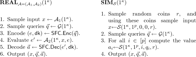
  We say that $\mathsf {SFC}$ is strongly spooky-free if there exists a ${\textsc {ppt}}$ simulator $\mathcal{S}$ such that for every ${\textsc {ppt}}$ adversary $\mathcal{A}$ the experiments ${{\varvec{REAL}}}_{\mathcal{A}}(1^\kappa )$ and ${{\varvec{SIM}}}{\mathcal{S}^\mathcal{A}}(1^\kappa )$ are computationally-indistinguishable. Similarly, we say that $\mathsf {SFC}$ is weakly spooky-free if the simulator can be chosen after the adversary and the distinguisher have been set.

On Black-Box Reductions of Spooky Free Compilers. Let us explicitly instantiate the definition of black box reductions (Definition 14 above) in the context of (weak) spooky free compilers. This is the definition that will be used to prove our main technical result in Theorem 20.

Consider a candidate spooky free compiler as in Definition 17 above. Then a pair of (not necessarily efficient) algorithms $(\mathcal{A}, \varPsi )$ breaks weak spooky freeness if for any simulator $\mathcal{S}$ (possibly dependent on $\mathcal{A}, \varPsi$) allowed to run in time $\mathrm{poly}(\mathsf {time}(\mathcal{A}), \mathsf {time}(\varPsi ))$, it holds that $\varPsi$ can distinguish between the distributions $\mathbf{REAL }_{\mathcal{A}}$ and $\sim {\mathcal{S}}$ with non-negligible probability (we refer to this as “breaking spooky freeness”).

A black-box reduction from a falsifiable assumption $(\mathcal{C},\eta )$ to a weakly spooky free compiler is an oracle machine $\mathcal{R}$ that, given oracle access to a pair of machines $(\mathcal{A}, \varPsi )$ that break weak spooky freeness as defined above, $\mathcal{R}^{(\mathcal{A}, \varPsi )}$ has non-negligible advantage against $(\mathcal{C},\eta )$. We note that we will prove an even stronger result that places no computational restrictions at all on the running time of $\mathcal{S}$.

4 Non-Succinct Spooky Freeness Is Trivial

In this section, we construct a non-succinct spooky free FHE, where the length of each ciphertext and the length of each public-key is exponential in the length of the messages. Specifically, we show how to convert any FHE scheme into a spooky-free FHE scheme such that the length of each ciphertext and each public key is $2^k\cdot \mathrm{poly}(\lambda )$, where k is the length of the messages.

We note that a spooky-free FHE is stronger than a spooky-free compiler, since the latter is tied to a specific MIP whereas the former is “universal”.

Theorem 18

There exists an efficient generic transformation from any fully-homomorphic encryption scheme $\mathrm {FHE}= (\mathsf {FHE.Keygen},\mathsf {FHE.Enc},\mathsf {FHE.Dec},\mathsf {FHE.Eval})$ into a scheme $\mathrm {FHE}^\prime = (\mathsf {FHE.Keygen}^\prime ,\mathsf {FHE.Enc}^\prime ,\mathsf {FHE.Dec}^\prime ,\mathsf {FHE.Eval}^\prime )$ that is fully-homomorphic and strongly spooky-free. The length of each ciphertext generated by $\mathsf {FHE.Enc}^\prime$ and the length of each public-key generated by $\mathsf {FHE.Keygen}^\prime$ is $2^k\cdot \mathrm{poly}(\lambda )$, where k is the length of each message.

Proof Overview. We transform the scheme to have equivocal properties. Specifically, the transformed scheme’s ciphertexts can be replaced with ones that can be decrypted to any value using different pre-computed secret-keys. The joint distribution of each secret-key and the special ciphertext are indistinguishable from a properly generated secret-key and ciphertext. This allows us to define a simulator that precomputes those secret-keys and queries the adversary using an equivocable ciphertext. Then, it decrypts with the secret-key corresponding to the given message to extract the adversary’s answers. By indistinguishability, this is the same answer that would be produced by querying the adversary, if it was queried with an encryption of that message.

We achieve this property by simply generating independently $2^k$ public-keys, whereas the secret-key corresponds only to one of the public-keys. Each ciphertext is $2^k$ encryptions, under each public-key. The equivocable ciphertext is produced by encrypting each of the $2^k$ possible messages under some public-key, in a randomly chosen order. Indistinguishability follows from the semantic-security of the original scheme.

Remark 19

We assume, without the loss of generality, that the length of an encryption of k bits is bounded by $k \cdot \mathrm{poly}(\lambda )$, since we can always encrypt bit-by-bit while preserving security and homomorphism.

Proof

Let $k = k(\lambda )$ be an upper-bound on the length of the messages $\left| {m_i} \right| \le k$, where $(m_1,\ldots ,m_n,\alpha ) \leftarrow \mathcal{D}$. We define the scheme $\mathrm {FHE}^\prime$ as follows:

• $\mathsf {FHE.Keygen}^\prime (1^\lambda )$: Generate $2^k$ pairs of keys $( \mathsf {pk}_i, \mathsf {sk}_i) \leftarrow \mathsf {FHE.Keygen}(1^\lambda )$. Then, choose uniformly at random a n index $j {\mathop {\leftarrow }\limits ^{\scriptscriptstyle {\$}}}[2^k]$, and output $(\vec { \mathsf {pk}}, ( \mathsf {sk}_j, j))$.

• $\mathsf {FHE.Enc}^\prime (\vec { \mathsf {pk}}, \mu )$: Encrypt the message under each public-key $c_i \leftarrow \mathsf {FHE.Enc}( \mathsf {pk}_i, \mu )$, then output $\vec {c}$.

• $\mathsf {FHE.Dec}^\prime (( \mathsf {sk}, j), \vec {\hat{c}})$: Decrypt according to the indexed secret-key and output $\mu ' {:=}\mathsf {FHE.Dec}( \mathsf {sk}, \hat{c}_j)$.

• $\mathsf {FHE.Eval}^\prime (\vec { \mathsf {pk}},\vec {c}, \mathcal{C})$: For every $i \in [2^k]$ compute $\hat{c}_i \leftarrow \mathsf {FHE.Eval}( \mathsf {pk}_i, c_i, \mathcal{C})$ and output $\vec {\hat{c}}$.

Clearly $\mathrm {FHE}^\prime$ is a fully-homomorphic encryption scheme. It is thus left to prove that it is strongly spooky-free.

The simulator $\mathcal{S}^{\mathcal{A}}(1^\lambda ,1^n,i,m_i;r)$ First, the simulator uses its randomness r to sample $n \cdot 2^k$ pairs of keys $( \mathsf {pk}_{\ell , j}, \mathsf {sk}_{\ell , j}) \leftarrow \mathsf {FHE.Keygen}(1^\lambda ), \ell \in [n], j \in [2^k]$. Then, for every $2^k$-tuple $\vec { \mathsf {pk}}_\ell = ( \mathsf {pk}_{\ell , 1}, \ldots , \mathsf {pk}_{\ell , 2^k})$, it chooses a permutation $\pi _\ell : [2^k] \rightarrow [2^k]$, encrypts the message ${\pi _\ell }^{-1}(j)$ under the public-key $\mathsf {pk}_{\ell ,j}$, for every $j \in \{0,1\}^k$

$$ c_{\ell , j} = \mathsf {FHE.Enc}( \mathsf {pk}_{\ell , j}, {\pi _\ell }^{-1}(j))~. $$

Next, it sets $\vec {c}_\ell = (c_{\ell , 1}, \ldots , c_{\ell , 2^k})$ and queries the adversary to get $(\vec {c'}_1,\ldots ,\vec {c'}_n) \leftarrow \mathcal{A}((\vec { \mathsf {pk}}_1,\ldots ,\vec { \mathsf {pk}}_n),(\vec {c}_1,\ldots ,\vec {c}_n))$. Finally it outputs $m^\prime _i {:=}\mathsf {FHE.Dec}( \mathsf {sk}_{i,{\pi }_\ell (m_i)}, c'_{i,{\pi }_\ell (m_i)})$.

Claim 1

For every ${\textsc {ppt}}$ adversary $\mathcal{A}$ and distribution $\mathcal{D}$, the experiments ${{\varvec{REAL}}}_{\mathcal{D},\mathcal{A}}$ and ${{\varvec{SIM}}}_{\mathcal{D},\mathcal{S}^{\mathcal{A}}}$ are computationally indistinguishable.

Proof

We prove using a sequence of hybrids.

• $\mathcal {H}_0$: This is simply the distribution $\mathbf{REAL }_{\mathcal{D},\mathcal{A}}$.

• $\mathcal {H}_{1, i}$ $(i \in [n])$: In these hybrids we modify the key generation step in $\mathbf{REAL }_{\mathcal{D},\mathcal{A}}$: Instead of choosing $j_i {\mathop {\leftarrow }\limits ^{\scriptscriptstyle {\$}}}[2^k]$ uniformly at random, we choose uniformly at random a permutation $\pi _i : [2^k] \rightarrow [2^k]$ and set $j_i = {\pi }_i(m_i)$. These hybrids are identically distributed, since the $\pi _i$’s are random permutations, so each $j_i$ is distributed uniformly over $[2^k]$.

• $\mathcal {H}_{2, i, j}$ $(i \in [n], j \in [2^k])$: In these hybrids we modify the encryption step in $\mathbf{REAL }_{\mathcal{D},\mathcal{A}}$: Instead of letting $c_{i, j} \leftarrow \mathsf {FHE.Enc}( \mathsf {pk}_{i, j}, m_i)$, set $c_{i, \pi _i(j)} \leftarrow \mathsf {FHE.Enc}( \mathsf {pk}_{i, \pi _i(j)}, j)$, where $\pi _i$ is the permutation from the previous hybrids. These hybrids are computationally indistinguishable by the semantic security of $\mathsf {FHE}$.

Finally, note that $\mathcal {H}_{2, n, 2^k}$ is actually $\mathbf{SIM }_{\mathcal{D},\mathcal{S}^{\mathcal{A}}}$. This is since for every $i \in [n]$, the simulator queries the adversary the same query every time, and that query is distributed as the one in $\mathcal {H}_{2, n, 2^k}$. Moreover, the adversary’s answer is decrypted in the same manner both in $\mathbf{SIM }_{\mathcal{D},\mathcal{S}^{\mathcal{A}}}$ and $\mathcal {H}_{2, n, 2^k}$. Thus $\mathbf{REAL }_{\mathcal{D},\mathcal{A}} {\ {\mathop {\approx }\limits ^{c}}\ }\mathbf{SIM }_{\mathcal{D},\mathcal{S}^{\mathcal{A}}}$, as desired.

5 Succinct Spooky Freeness Cannot Be Proven Using a Black-Box Reduction

We state and prove our main theorem.

Theorem 20

Let $\varPi = (\mathcal{G}, \vec {\mathcal{P}}, \mathcal{V})$ be a succinct one-round MIP for L. Let $\mathsf {SFC}= (\mathsf {SFC.Enc}, \mathsf {SFC.Dec}, \mathsf {SFC.Eval})$ be a spooky-free compiler for $\varPi$, with $\left| {e'} \right| = \mathrm{poly}(\kappa ) \cdot \left| {x} \right| ^{\alpha '}$ for some $\alpha ' < 1$. Finally, let $(\mathcal{C}, \eta )$ be a falsifiable assumption.

Then, assuming the existence of a language L with a sub-exponentially hard subset-membership problem $(\mathcal{L},\overline{\mathcal{L}},\mathsf{Sam})$ with hardness parameter $\alpha > \alpha '$, there is no black-box reduction showing the weakly spooky-freeness of $\mathsf {SFC}$ based on the assumption $(\mathcal{C}, \eta )$, unless $(\mathcal{C}, \eta )$ is polynomially solvable.

Proof Overview. We start by defining an inefficient adversary $(\overline{\mathcal{A}}, \overline{\varPsi })$ against $\mathsf {SFC}$, or more precisely a distribution over adversaries specified by a family of sets $\overline{X}$. These sets contain, for each value of the security parameter $1^\kappa$ a large number of inputs from $\overline{\mathcal{L}}$ of length $n=\mathrm{poly}(\kappa )$ for a sufficiently large polynomial to make $|e'|$ bounded by $n^{\alpha }$. The adversary $\overline{\mathcal{A}}$ picks a random x from the respective set and generates a response $e'$ as follows. As a thought experiment, if it was the case that $x\in \mathcal{L}$, then $\mathsf {SFC}$ allows us to generate $e'$ that will be accepted by the MIP verifier. Therefore, the Dense Model Theorem states that it is possible to generate a computationally indistinguishable $e'$ also for $x \in \overline{\mathcal{L}}$. The distinguisher $\overline{\varPsi }$ will check that x is indeed in the respective set of $\overline{X}$ and if so, it will apply the MIP verifier. The soundness of MIP guarantees that this distribution cannot be simulated by independent provers. Note that the phase where $\overline{\varPsi }$ checks that indeed $x \in \overline{X}$ is critical since otherwise the simulator could produce $x \in \mathcal{L}$ which will cause $\overline{\varPsi }$ to accept! The use of a common $\overline{X}$ allows $\overline{\mathcal{A}}$ and $\overline{\varPsi }$ to share a set of inputs for which they know the simulator cannot work.

Since $(\overline{\mathcal{A}}, \overline{\varPsi })$ is successful against $\mathsf {SFC}$, it means that the reduction breaks the assumption given oracle access to $(\overline{\mathcal{A}}, \overline{\varPsi })$.⁷ Our goal now is to show an efficient procedure $(\mathcal{A}, \varPsi )$ which is indistinguishable from $(\overline{\mathcal{A}}, \overline{\varPsi })$ in the eyes of the reduction. This will show that the underlying assumption is in fact polynomially solvable.

To do this, we notice that the reduction can only ever see polynomially many x’s, so there is no need to sample a huge set $\overline{X}$, and an appropriately defined polynomial subset would be sufficient. Furthermore, instead of sampling from $\overline{\mathcal{L}}$, we can sample from $\mathcal{L}$ together with a witness, and compute $e'$ as a legitimate $\mathsf {SFC}.\mathsf {Eval}$ response. The Dense Model Theorem ensures that this strategy will be indistinguishable to the reduction, and therefore it should still be successful in breaking the assumption. Note that we have to be careful since the reduction might query its oracle on tiny security parameter values for which n is not large enough to apply the Dense Model Theorem. For those small values we create a hard-coded table of adversary responses (since these are tiny values, the table is still not too large).

Finally, we see that our simulated adversary runs in polynomial time since it only needs to sample from $\mathcal{L}$, which is efficient using $\mathsf{Sam}$, and use the witness to compute $e'$ via $\mathsf {SFC}.\mathsf {Eval}$. We conclude that we have a polynomial time algorithm that succeeds in breaking the assumption, as required in the theorem.

Proof

We proceed as in the sketch above. By the properties of $\mathsf {SFC}$ as stated in the theorem, there exist constants $\beta _1, \beta _2, \beta _3 > 0$ such that $\beta _1=\alpha -\alpha '$, $\left| {e'} \right| \le O(\kappa ^{\beta _2} \cdot \left| {x} \right| ^{\alpha - \beta _1})$, $\left| {e} \right| \le \kappa ^{\beta _3}$. We define

$$n(\kappa ) \triangleq \kappa ^{\max \{2\beta _2 / \beta _1, \beta _3/\alpha '\}}~,$$

and note that $\left| {e} \right| , \left| {e'} \right| = o(n^\alpha )$, when $\left| {x} \right| = n(\kappa )$.

Proofs Can Be Spoofed. We start by showing how to inefficiently spoof $\mathsf {SFC}$ answers for non-accepting inputs. Consider an encoded query e for $\mathsf {SFC}$ w.r.t. security parameter $1^\kappa$, and define the distribution $(\mathcal{L}, \mathcal{E})$ as follows:

• 1. Sample $(x, w) \leftarrow \mathsf{Sam}(1^{n(\kappa )})$.

• 2. Evaluate $e' \leftarrow \mathsf {SFC.Eval}(e, x, w)$.

• 3. Output $(x, e')$.

The following claim shows that it is possible to sample from a distribution that is computationally indistinguishable distribution from $(\mathcal{L}, \mathcal{E})$, but where the first component comes from $\overline{\mathcal{L}}$.

Claim 2

For every e, there exists a randomized function $h=h_e$ such that the distributions $(\mathcal{L}, \mathcal{E})$ and $(\overline{\mathcal{L}}, h(\overline{\mathcal{L}}))$ are $(2\cdot 2^{-n^\alpha }, 2^{n^\alpha })$ indistinguishable.

Proof

Follows from Corollary 7 since $\mathcal{L}_n$ and $\overline{\mathcal{L}}_n$ are $\alpha$-sub-exponentially indistinguishable. $\blacksquare$

Constructing a Spooky Adversary. We define an adversary $\overline{\mathcal{A}}$, along with a distinguisher $\overline{\varPsi }$ for the spooky-free experiment in $\mathsf {SFC}$. We note that both $\overline{\mathcal{A}}$ and $\overline{\varPsi }$ are inefficient algorithms, and more precisely, they are distributions over algorithms.

For every value of $\kappa$, define $\nu (\kappa ) = 2^{0.1 \cdot n(\kappa )^\alpha }$. Define a vector $\overline{X}_{n(\kappa )} {\mathop {\leftarrow }\limits ^{\scriptscriptstyle {\$}}}\overline{\mathcal{L}}^{\otimes \nu (\kappa )}_{n(\kappa )}$, i.e. a sequence of independent samples from $\overline{\mathcal{L}}_n$. The functionality of $\overline{\mathcal{A}}$ and $\overline{\varPsi }$ is as follows:

• $\overline{\mathcal{A}}(1^\kappa , e)$: Samples $i \in [\nu (\kappa )]$, sets $\bar{x} {\mathop {\leftarrow }\limits ^{\scriptscriptstyle {\$}}}\overline{X}_{n(\kappa )}[i]$ (i.e. the i’th element in the vector), and outputs $h(\bar{x})$.

• $\overline{\varPsi }(1^\kappa , x,\vec {q}, \vec {a})$: Outputs 1 if and only if $x \in \overline{X}_{n(\kappa )}$ and $\mathcal{V}(\vec {q}, \vec {a}, x) = 1$ .

The following claim asserts that the adversary $\overline{\mathcal{A}}$ and the distinguisher $\overline{\varPsi }$ win the spooky-freeness game for the compiler $\mathsf {SFC}$ with probability 1 over the choice of the respective $\overline{X}= \{\overline{X}_{n(\kappa )}\}_{\kappa }$.

Claim 3

With probability 1 over the choice of $\overline{X}= \{\overline{X}_{n(\kappa )}\}_{\kappa }$ it holds that $(\overline{\mathcal{A}}, \overline{\varPsi })$ has non-negligible advantage in the spooky freeness game against $\mathsf {SFC}$ with any (possibly computationally unbounded) simulator.

Proof

Let $\sigma$ denote the soundness of the underlying MIP system. According to the definition of an MIP (see Definition 3), the soundness gap, $\sigma _{\text {gap}}\triangleq 1-\sigma$, is non-negligible.

We start by showing that for all $\overline{X}$, any value of $\kappa$, and any (possibly unbounded) spooky-free simulator $\mathcal{S}$ for the compiler $\mathsf {SFC}$, it holds that

$$ \Pr [\overline{\varPsi }(\mathbf{SIM }_{\mathcal{S}}(1^\kappa ))=1| \overline{X}] \le \sigma (\kappa ). $$

This follows since by the definition of the simulator, each value of its random string r defines an input x and induces a sequence of algorithms $\vec {\mathcal{S}}$ where

$$ (\mathcal{S}_1(q_1), \ldots , \mathcal{S}_p(q_p)) = \vec {\mathcal{S}}(\vec {q})~. $$

If the induced $x \not \in {\overline{X}_{n(\kappa )}}$ then $\overline{\varPsi }$ will output 0. If $x \in {\overline{X}_{n(\kappa )}}$ then by the soundness of $\varPi$, the probability that the verifier $\mathcal{V}$ accepts answers generated by $\vec {\mathcal{S}}$ is at most $\sigma (\kappa )$, and thus $\overline{\varPsi }$ outputs 1 with probability at most $\sigma (\kappa )$.

Next, we turn to show that $\Pr [\overline{\varPsi }(\mathbf{REAL }_{\overline{\mathcal{A}}}(1^\kappa ))=1 | \overline{X}]$ is bounded away from $\sigma (\kappa )$ with probability 1 on $\overline{X}$. To this end, we define a sequence of events $\{E_\kappa \}_{\kappa \in {\mathbb N}}$, where $E_\kappa$ is the event that

$$\Pr [\overline{\varPsi }(\mathbf{REAL }_{\overline{\mathcal{A}}}(1^\kappa ))=1 | \overline{X}] \le 1-\sigma _{\text {gap}}(\kappa )/2~,$$

where the probability is over everything except the choice of $\overline{X}$. We show that with probability 1 over the choice of $\overline{X}$, only finitely many of the events $E_\kappa$ occur.

To see this, fix queries $\vec {q} \leftarrow \mathcal{G}(1^\kappa )$ and encoding $(e, \mathsf {dk}) \leftarrow \mathsf {SFC.Enc}(\vec {q})$ for the experiment $\mathbf{REAL }_{\overline{\mathcal{A}}}$. Note that since the compiler’s decoding algorithm $\mathsf {SFC.Dec}$ can be described by a $\mathrm{poly}(\kappa )$ sized circuit, then we can describe the MIP’s verifier $\mathcal{V}$ as a $\mathrm{poly}(\kappa )$ sized circuit that takes inputs from $(\overline{\mathcal{L}}, h(\overline{\mathcal{L}}))$.

Recall that by Claim 2, the distributions $(\mathcal{L}, \mathcal{E})$ and $(\overline{\mathcal{L}}, h(\overline{\mathcal{L}}))$ are $(2\cdot 2^{-n^\alpha }, 2^{n^\alpha })$-indistinguishable. Moreover, by the completeness of the MIP, $\mathcal{V}$ outputs 1 with probability $1$ on inputs from $(\mathcal{L}, \mathcal{E})$. We conclude that $\mathcal{V}$ accepts inputs from $(\overline{\mathcal{L}}, h(\overline{\mathcal{L}}))$ with overwhelming probability, and therefore $\overline{\varPsi }$ also accepts with overwhelming probability inputs from $\mathbf{REAL }_{\overline{\mathcal{A}}}$. In other words, we have that

$$ \mathop {{\mathbb E}}_{\overline{X}}\left[ \Pr [\overline{\varPsi }(\mathbf{REAL }_{\overline{\mathcal{A}}}(1^\kappa ))=1 | \overline{X}]\right] \ge 1-\mathrm{negl}(\kappa )~. $$

By a Markov argument this implies that

$$ \mathop {\Pr }_{\overline{X}}\left[ \Pr [\overline{\varPsi }(\mathbf{REAL }_{\overline{\mathcal{A}}}(1^\kappa ))=1 | \overline{X}] \le 1-\sigma _{\text {gap}}(\kappa )/2\right] \le \mathrm{negl}(\kappa )~. $$

Finally, we apply the Borel-Cantelli Lemma to conclude that with probability 1 over the choice of $\overline{X}$, only finitely many of the events $E_\kappa$ occur, as desired.

Thus, with probability 1 (over the choice of $\overline{X}$), it holds that $(\overline{\mathcal{A}}, \overline{\varPsi })$ has advantage at least $\sigma _{\text {gap}}/2$ in the spooky free game. This completes the proof of the claim. $\blacksquare$

Fooling the Reduction. We now notice that by Corollary 15, it is sufficient to prove the theorem for $\eta =0$. Assume that there exists a black-box reduction $\mathcal{R}$ as in the theorem statement, and we will prove that $(\mathcal{C}, 0)$ is solvable in polynomial time. We notice that since $(\overline{\mathcal{A}}, \overline{\varPsi })$ break spooky freeness with probability 1, it follows from Lemma 16 that

$$\begin{aligned} \delta (\lambda ) = \Pr [\mathcal{R}^{(\overline{\mathcal{A}}, \overline{\varPsi })}(1^\lambda ) \text { wins } \mathcal{C}(1^\lambda )] \end{aligned}$$

is noticeable, where the probability is taken over the randomness of sampling $(\overline{\mathcal{A}}, \overline{\varPsi })$, the randomness of the reduction and the randomness of $\mathcal{C}$.

We turn to define another adversary $\mathcal{A}$ and distinguisher $\varPsi$, by modifying $\overline{\mathcal{A}}$ and $\overline{\varPsi }$ in a sequence of changes. Our goal is to finally design $\mathcal{A}, \varPsi$ computable in $\mathrm{poly}(\lambda )$ time, while ensuring that $\mathcal{R}^{(\mathcal{A}, \varPsi )}$ still has advantage $\varOmega (\delta )$.

Hybrid ${\mathcal {H}_{0}}$. In this hybrid we execute $\mathcal{R}^{(\overline{\mathcal{A}}, \overline{\varPsi })}$ as defined.

$$ \delta (\lambda ) = \mathop {\Pr }_{\mathcal {H}_{0}}[\mathcal{R}^{(\overline{\mathcal{A}}, \overline{\varPsi })}(1^\lambda ) \text { wins } \mathcal{C}(1^\lambda )]~. $$

Hybrid ${\mathcal {H}_{1}}$. Let $\kappa _{\max }= \kappa _{\max }(\lambda ) = \mathrm{poly}(\lambda )$ be a bound on the size of the security parameters that the reduction $\mathcal{R}$ uses when interacting with its oracle. Note that $\kappa _{\max }$ is bounded by the runtime of the reduction, which in turn is bounded by some fixed polynomial (in $\lambda$). In this step, we remove all the sets relative to $\kappa > \kappa _{\max }$ from the ensemble $\{\overline{X}_{n(\kappa )}\}$. That is, now $\{\overline{X}_{n(\kappa )}\}$ only contains finite (specifically $\mathrm{poly}(\lambda )$) many sets. Since by definition $\mathcal{R}$ cannot query on such large values of $\kappa$ this step does not affect the advantage of $\mathcal{R}$.

$$ \left| {\mathop {\Pr }_{\mathcal {H}_{1}}[\mathcal{R}^{(\overline{\mathcal{A}}, \overline{\varPsi })}(1^\lambda ) \text { wins } \mathcal{C}(1^\lambda )] - \mathop {\Pr }_{\mathcal {H}_{0}}[\mathcal{R}^{(\overline{\mathcal{A}}, \overline{\varPsi })}(1^\lambda ) \text { wins } \mathcal{C}(1^\lambda )] } \right| = 0~. $$

Hybrid ${\mathcal {H}_{2}}$. Let $\kappa _{\min }= \kappa (\lambda )$ be the maximal $\kappa$ such that $2^{n(\kappa )^{\alpha }} \le \lambda ^c$ for a constant c to be selected large enough to satisfy constraints that will be explained below. Note that for all $\kappa \le \kappa _{\min }$ it holds that $\nu (\kappa ) = |\overline{X}_{n(\kappa )}| = 2^{O(n^{\alpha })} = \mathrm{poly}(\lambda )$ and for all $\kappa > \kappa _{\min }$ it holds that $\nu (\kappa ) = 2^{0.1 \cdot n^{\alpha }} \ge \lambda ^{0.1 c}$.

From here on, we will focus on $\kappa \in (\kappa _{\min }, \kappa _{\max })$, since in the other regimes we can indeed execute $\overline{\mathcal{A}}, \overline{\varPsi }$ efficiently. We call this the relevant domain.

We now change $\overline{\mathcal{A}}$ and make it stateful. Specifically, for all $\kappa \in (\kappa _{\min }, \kappa _{\max })$, instead of randomly selecting an $\bar{x} \in \overline{X}_{n(\kappa )}$ for every invocation, we go over the elements of $\overline{X}_{n(\kappa )}$ in order.

Claim 4

If c is chosen so that $t(\lambda )^2/\lambda ^{0.1 c} \le \delta /10$ then

$$ \left| \mathop {\Pr }_{\mathcal {H}_{2}}[\mathcal{R}^{(\overline{\mathcal{A}}, \overline{\varPsi })}(1^\lambda ) \text { wins } \mathcal{C}(1^\lambda )] - \mathop {\Pr }_{\mathcal {H}_{1}}[\mathcal{R}^{(\overline{\mathcal{A}}, \overline{\varPsi })}(1^\lambda ) \text { wins } \mathcal{C}(1^\lambda )] \right| \le \delta /10~. $$

Proof

The view of $\mathcal{R}$ can only change in the case where the same index i was selected more than once throughout the executions of $\overline{\mathcal{A}}$ on $\kappa > \kappa _{\min }$. Since $\mathcal{R}$ makes at most t queries, this event happens with probability at most $t^2 / \nu (\kappa _{\min }) \le t(\lambda )^2/\lambda ^{c \cdot \gamma }$. If we choose c as in the claim statement, the probabilistic distance follows.$\blacksquare$

Hybrid ${\mathcal {H}_{3}}$. We now change $\overline{\varPsi }$ to also be stateful, and in fact its state is joint with $\overline{\mathcal{A}}$. Specifically for the relevant domain $\kappa \in (\kappa _{\min }, \kappa _{\max })$, instead of checking whether $x \in {\overline{X}_{n(\kappa )}}$, it only checks whether x is in the prefix of ${\overline{X}_{n(\kappa )}}$ that had been used by $\overline{\mathcal{A}}$ so far.

Claim 5

If c is chosen so that $t(\lambda ) \cdot \lambda ^{-0.9 c} \le \delta /10$ then

$$ \left| \mathop {\Pr }_{\mathcal {H}_{3}}[\mathcal{R}^{(\overline{\mathcal{A}}, \overline{\varPsi })}(1^\lambda ) \text { wins } \mathcal{C}(1^\lambda )] - \mathop {\Pr }_{\mathcal {H}_{2}}[\mathcal{R}^{(\overline{\mathcal{A}}, \overline{\varPsi })}(1^\lambda ) \text { wins } \mathcal{C}(1^\lambda )] \right| \le \delta /10~. $$

Proof

We note that if $\mathcal{R}$ only makes $\overline{\varPsi }$ queries for these $\kappa$ values with x inputs that are either in the prefix of ${\overline{X}_{n(\kappa )}}$ or not in ${\overline{X}_{n(\kappa )}}$ at all, then its view does not change. Let us consider the first $\overline{\varPsi }$ query of $\mathcal{R}$ that violates the above. Since this is the first such query, the view of $\mathcal{R}$ so far only depends on the relevant prefixes of ${\overline{X}_{n(\kappa )}}$’s. Let x be the value queried by $\mathcal{R}$ and let us bound the probability that x is in the suffix of ${\overline{X}_{n(\kappa )}}$ for the respective $\kappa$. Recall that the length of the suffix is at most $\nu (\kappa )$.

Since the view of $\mathcal{R}$ so far, and therefore x, is independent of this suffix, we can consider a given x and bound the probability that some entry in the suffix hits x. By Lemma 5, the entropy of each entry in ${\overline{X}_{n(\kappa )}}$ is at least $n^{\alpha }$, which means that each value hits x with probability at most $2^{-n^{\alpha }}$. Applying the union bound we get a total probability of at most $\nu (\kappa ) \cdot 2^{-n(\kappa )^{\alpha }} = 2^{-0.9 n(\kappa )^{\alpha }}$. Since $\kappa > \kappa _{\min }$ we get that this probability is at most $\lambda ^{-0.9 c}$.

Applying the union bound over all at most t queries of $\mathcal{R}$, the probability that the above is violated for any of them is at most $t \cdot \lambda ^{-0.9 c}$ and the claim follows. $\blacksquare$

Hybrid ${\mathcal {H}_{4}}$. We now change $\overline{\mathcal{A}}, \overline{\varPsi }$ in the relevant domain to sample the values of $\bar{x}$ on the fly rather than have them predetermined ahead of time. Specifically, ${\overline{X}_{n(\kappa )}}$ is initialized as an empty vector in the relevant domain. Whenever a query to $\overline{\mathcal{A}}$ is made relative to such a $\kappa$, $\overline{\mathcal{A}}$ samples a fresh $\bar{x} {\mathop {\leftarrow }\limits ^{\scriptscriptstyle {\$}}}\overline{\mathcal{L}}_{n(\kappa )}$, and applies $h_e$ to it to compute the response $e'$. The sampled $\bar{x}$ is then appended to ${\overline{X}_{n(\kappa )}}$. When the distinguisher $\overline{\varPsi }$ is called, it uses the current value of ${\overline{X}_{n(\kappa )}}$ for its execution. Note that this change does not change the view of $\mathcal{R}$ at all.

$$ \left| \mathop {\Pr }_{\mathcal {H}_{4}}[\mathcal{R}^{(\overline{\mathcal{A}}, \overline{\varPsi })}(1^\lambda ) \text { wins } \mathcal{C}(1^\lambda )] - \mathop {\Pr }_{\mathcal {H}_{3}}[\mathcal{R}^{(\overline{\mathcal{A}}, \overline{\varPsi })}(1^\lambda ) \text { wins } \mathcal{C}(1^\lambda )] \right| = 0~. $$

Hybrid $\mathcal {H}_{5}$. Now instead of sampling $\bar{x} {\mathop {\leftarrow }\limits ^{\scriptscriptstyle {\$}}}\overline{\mathcal{L}}_n$ and evaluating $h_e$ on it, $\overline{\mathcal{A}}$ instead samples $(x,w) {\mathop {\leftarrow }\limits ^{\scriptscriptstyle {\$}}}\mathsf{Sam}(1^n)$ and computes $e'$ by running $e' \leftarrow \mathsf {SFC.Eval}(e, x, w)$. The value x is appended to ${\overline{X}_{n(\kappa )}}$ just as before and the behavior of $\overline{\varPsi }$ does not change.

We would like to prove that this does not change the winning probability using a hybrid. Specifically, go over all samples of $\bar{x}$ and apply Corollary 7 to argue indistinguishability, but we need to be careful since indistinguishability only holds against adversaries of size $2^{O(n^\alpha )}$ but for the smaller values of $\kappa$ in the relevant domain this is not necessarily the case. We will therefore need the following claim.

Claim 6

Let $\hat{\kappa }\in (\kappa _{\min }, \kappa _{\max })$ and let $\hat{n}= n(\hat{\kappa })$. Then the functionality of $(\overline{\mathcal{A}}, \overline{\varPsi })_{\mathcal {H}_{4}}$ on all $\kappa \le \hat{\kappa }$ is computable by a size $2^{O(\hat{n}^{\alpha })}$ circuit.

Proof

We note that for all $\kappa$, $\overline{\mathcal{A}}$ takes inputs e of length at most $o(n^{\alpha })$ and outputs $e'$ of length at most $o(n^{\alpha })$. We can therefore completely define its functionality using a table of size $2^{o(n^\alpha )}$. In addition to this truth table, we can also pre-sample ${\overline{X}_{n(\kappa )}}$. For $\kappa \le \kappa _{\min }$, the set ${\overline{X}_{n(\kappa )}}$ contains at most $\nu (\kappa ) \le \nu (\hat{\kappa }) = 2^{0.1 \cdot \hat{n}^\alpha }$ samples, and for $\kappa > \kappa _{\min }$ it contains at most $t(\lambda ) = \mathrm{poly}(\lambda ) \le 2^{(1/c) \cdot O(\hat{n}^\alpha )}$ samples. Using these sets, we can simulate on-line sampling by going over these samples one by one. Taking the sum of table sizes for all $\kappa \le \hat{\kappa }$, the claim follows. $\blacksquare$

This will allow us to prove a bound on the difference between the hybrids.

Claim 7

If c is chosen so that $t(\lambda )^2 \cdot \lambda ^{-c} \le \delta /10$ then

$$ \left| \mathop {\Pr }_{\mathcal {H}_{5}}[\mathcal{R}^{(\overline{\mathcal{A}}, \overline{\varPsi })}(1^\lambda ) \text { wins } \mathcal{C}(1^\lambda )] - \mathop {\Pr }_{\mathcal {H}_{4}}[\mathcal{R}^{(\overline{\mathcal{A}}, \overline{\varPsi })}(1^\lambda ) \text { wins } \mathcal{C}(1^\lambda )] \right| \le \delta /10~. $$

Proof

The proof uses a hybrid argument. In hybrid $(j_1, j_2)$, we construct the circuit from Claim 6 with respect to $\hat{\kappa }= \kappa _{\max }-j_1$, whose size is $2^{O(\hat{n}^{\alpha })}$. We use this circuit to answer all queries for $\kappa < \hat{\kappa }$, as well as the first $t-j_2$ queries for $\kappa = \hat{\kappa }$. The rest of the queries are answered as in $\mathcal {H}_{5}$ by sampling x, w. The Distinguisher answers consistently with the x’s that were used by $\overline{\mathcal{A}}$.

One can see that taking $j_1 = 0$, $j_2=0$, we get a functionality that is identical to $\mathcal {H}_{4}$, and taking $j_1 = \kappa _{\max }-\kappa _{\min }$, $j_2 = 0$ we get a functionality identical to $\mathcal {H}_{5}$. Furthermore, the functionality with $(j_1, t)$ is identical to the functionality with $(j_1+1, 0)$. Now consider the difference between hybrids $(j_1, j_2)$ and $(j_1, j_2+1)$. The only difference is whether $(x,e')$ is generated by sampling $x {\mathop {\leftarrow }\limits ^{\scriptscriptstyle {\$}}}\overline{\mathcal{L}}$ and $e' = h_e(x)$, or whether $(x,w) {\mathop {\leftarrow }\limits ^{\scriptscriptstyle {\$}}}\mathsf{Sam}(1^n)$ and $e' \leftarrow \mathsf {SFC.Eval}(e, x, w)$. Furthermore, in this hybrid $\mathcal{R}^{(\overline{\mathcal{A}}, \overline{\varPsi })}$ can be computed by a size $2^{O(n^{\alpha })}$ circuit. Corollary 7 implies that $\Pr [\mathcal{R}^{(\overline{\mathcal{A}}, \overline{\varPsi })}(1^\lambda ) \text { wins } \mathcal{C}(1^\lambda )]$ changes by at most $2\cdot 2^{-n^{\alpha }} \le 2 \cdot 2^{-n(\kappa _{\min })^{\alpha }} \le \lambda ^{-c}$. The total number of hybrids is at most $\kappa _{\max }(\lambda ) \cdot t(\lambda )$, and recalling that $\kappa _{\max }(\lambda ) \le t(\lambda )$ the claim follows. $\blacksquare$

We note that if we choose c to be an appropriately large constant, the resulting $\overline{\mathcal{A}}, \overline{\varPsi }$ run in $\mathrm{poly}(\lambda )$ time and only use x values in $\mathcal{L}$. We therefore denote them by $\mathcal{A}, \varPsi$. This is formally stated below.

Claim 8

There exist $(\mathcal{A}, \varPsi )$ computable by $\mathrm{poly}(\lambda )$ circuit that implements an identical functionality to $(\overline{\mathcal{A}}, \overline{\varPsi })_{\mathcal {H}_{5}}$.

Proof

We define $(\mathcal{A}, \varPsi )$ as follows. Consider the circuit described in Claim 6 for $\hat{\kappa }= \kappa _{\min }$ and use it to answer queries with $\kappa \le \kappa _{\min }$. Note that the circuit size is $\mathrm{poly}(\lambda )$. Queries with $\kappa > \kappa _{\max }$ don’t need to be answered by $(\overline{\mathcal{A}}, \overline{\varPsi })_{\mathcal {H}_{5}}$. As for queries in the relevant domain, the computation of $(\overline{\mathcal{A}}, \overline{\varPsi })_{\mathcal {H}_{5}}$ for these values of $\kappa$ runs in polynomial time in $\kappa$ and therefore also in $\lambda$. $\square$

Conclusion. Combining the hybrids above, we get that $\mathcal{R}^{(\mathcal{A}, \varPsi )}$ is a $\mathrm{poly}(\lambda )$-time algorithm with advantage

$$ \mathsf {Adv}_{\mathcal{R}^{(\mathcal{A}, \varPsi )}}^{(\mathcal{C}, 0)}(1^\lambda ) \ge \delta - 3 \cdot \delta /10 = \varOmega (\delta )~. $$

That is, $\mathcal{R}^{(\mathcal{A}, \varPsi )}$ is a polynomial time algorithm that breaks the assumption $(\mathcal{C}, 0)$ as required. $\square$

References

Aiello, W., Bhatt, S., Ostrovsky, R., Rajagopalan, S.R.: Fast verification of any remote procedure call: short witness-indistinguishable one-round proofs for NP. In: Montanari, U., Rolim, J.D.P., Welzl, E. (eds.) ICALP 2000. LNCS, vol. 1853, pp. 463–474. Springer, Heidelberg (2000). doi:10.1007/3-540-45022-X_39
Arora, S., Lund, C., Motwani, R., Sudan, M., Szegedy, M.: Proof verification and the hardness of approximation problems. J. ACM 45(3), 501–555 (1998)
Arora, S., Safra, S.: Probabilistic checking of proofs: a new characterization of NP. J. ACM 45(1), 70–122 (1998)
Bitansky, N., Canetti, R., Chiesa, A., Goldwasser, S., Lin, H., Rubinstein, A., Tromer, E.: The hunting of the SNARK. IACR Cryptology ePrint Archive, 2014:580 (2014)
Bitansky, N., Canetti, R., Chiesa, A., Tromer, E.: From extractable collision resistance to succinct non-interactive arguments of knowledge, and back again. In: Proceedings of the 3rd Innovations in Theoretical Computer Science Conference, ITCS 2012, pp. 326–349 (2012)
Bitansky, N., Canetti, R., Chiesa, A., Tromer, E.: Recursive composition and bootstrapping for SNARKS and proof-carrying data. In: STOC, pp. 111–120. ACM (2013)
Babai, L., Fortnow, L., Lund, C.: Non-deterministic exponential time has two-prover interactive protocols. Comput. Complex. 1(1), 3–40 (1991)
Biehl, I., Meyer, B., Wetzel, S.: Ensuring the integrity of agent-based computations by short proofs. In: Rothermel, K., Hohl, F. (eds.) MA 1998. LNCS, vol. 1477, pp. 183–194. Springer, Heidelberg (1998). doi:10.1007/BFb0057658
49th Annual IEEE Symposium on Foundations of Computer Science, FOCS 2008, 25–28 October 2008, Philadelphia, PA. IEEE Computer Society, USA (2008)
Damgård, I., Faust, S., Hazay, C.: Secure two-party computation with low communication. In: Cramer, R. (ed.) TCC 2012. LNCS, vol. 7194, pp. 54–74. Springer, Heidelberg (2012). doi:10.1007/978-3-642-28914-9_4
Dodis, Y., Halevi, S., Rothblum, R.D., Wichs, D.: Spooky encryption and its applications. In: Robshaw, M., Katz, J. (eds.) CRYPTO 2016. LNCS, vol. 9816, pp. 93–122. Springer, Heidelberg (2016). doi:10.1007/978-3-662-53015-3_4
Dwork, C., Langberg, M., Naor, M., Nissim, K., Reingold, O.: Succinct proofs for NP and spooky interactions. Unpublished manuscript (2001)
Dziembowski, S., Pietrzak, K.: Leakage-resilient cryptography. In: 49th Annual IEEE Symposium on Foundations of Computer Science, FOCS 2008, 25–28 October 2008, Philadelphia, PA, USA [DBL08], pp. 293–302 (2008)
Gentry, C., Wichs, D.: Separating succinct non-interactive arguments from all falsifiable assumptions. In: Proceedings of the Forty-third Annual ACM Symposium on Theory Of Computing, pp. 99–108. ACM (2011)
Kalai, Y.T., Raz, R., Rothblum, R.D.: Delegation for bounded space. In: Boneh, D., Roughgarden, T., Feigenbaum, J., (eds) Symposium on Theory of Computing Conference, STOC 2013, Palo Alto, CA, USA, 1–4 June 2013, pp. 565–574. ACM (2013)
Kalai, Y.T., Raz, R., Rothblum, R.D.: How to delegate computations: the power of no-signaling proofs. In: STOC, pp. 485–494. ACM (2014)
Micali, S.: CS proofs (extended abstracts). In: 35th Annual Symposium on Foundations of Computer Science, Santa Fe, New Mexico, USA, 20–22 November 1994, pp. 436–453. IEEE Computer Society (1994)
Naor, M.: On cryptographic assumptions and challenges. In: Boneh, D. (ed.) CRYPTO 2003. LNCS, vol. 2729, pp. 96–109. Springer, Heidelberg (2003). doi:10.1007/978-3-540-45146-4_6
Reingold, O., Trevisan, L., Tulsiani, M., Vadhan, S.P.: Dense subsets of pseudorandom sets. In: 49th Annual IEEE Symposium on Foundations of Computer Science, FOCS 2008, 25–28 October 2008, Philadelphia, PA, USA [DBL08], pp. 76–85 (2008)
Vadhan, S., Zheng, C.J.: A uniform min-max theorem with applications in cryptography. In: Canetti, R., Garay, J.A. (eds.) CRYPTO 2013. LNCS, vol. 8042, pp. 93–110. Springer, Heidelberg (2013). doi:10.1007/978-3-642-40041-4_6
Acknowledgments
We wish to thank the Asiacrypt reviewers for the extremely thorough review process, and for their useful and enlightening comments that helped improve this manuscript significantly.
Author information
Authors and Affiliations
Corresponding author
Editor information
Editors and Affiliations
Rights and permissions
Copyright information
© 2017 International Association for Cryptologic Research
About this paper
Cite this paper
Brakerski, Z., Kalai, Y.T., Perlman, R. (2017). Succinct Spooky Free Compilers Are Not Black Box Sound. In: Takagi, T., Peyrin, T. (eds) Advances in Cryptology – ASIACRYPT 2017. ASIACRYPT 2017. Lecture Notes in Computer Science(), vol 10626. Springer, Cham. https://doi.org/10.1007/978-3-319-70700-6_6
Download citation
DOI: https://doi.org/10.1007/978-3-319-70700-6_6
Published:
Publisher Name: Springer, Cham
Print ISBN: 978-3-319-70699-3
Online ISBN: 978-3-319-70700-6
eBook Packages: Computer ScienceComputer Science (R0)