An Improved Feature Selection Method for Target Discrimination in SAR Images

Abstract

Due to synthetic aperture radar (SAR) imaging principals, at particular azimuth or depression angle, targets and clutters may become very hard to distinguish, to solve this problem, many complicated features have been developed, this is not only a tough work, but little improvement of discrimination accuracy is obtained. In this paper, an improved target discrimination method is proposed, one-class quadratic discriminator (OCQD) has been used, compared with traditional method using Bayes discriminator, when number of features is limited, our new method has higher target classification correction than old methods, considering that target classification correction is more important than clutter classification correction, our proposed method has a good performance on target discrimination. First, discrimination scheme based on genetic algorithm (GA) is introduced. Second, feature extraction algorithms of SAR images have been introduced. Third, an improved feature selection method based on GA has been proposed, in which the OCQD has been used and a new fitness function has been designed. Finally, the theory of OCQD algorithm is explained. According to the experiment result based on moving and stationary target acquirement and recognition (MSTAR) database, our new method reduces target undetected rate by 1.5% compared to the state-of-the-art methods in target discrimination, besides, the efficiency of feature selection based on GA has been improved by 77%.

1 Introduction

Over past two decades, as the speed of synthetic aperture radar (SAR) imaging grow rapidly, knowledge based real-time interpretation of SAR image became harder and harder, development of SAR-ATR (automatic target recognition) system has become a hot area. A typical synthetic aperture radar (SAR) automatic target recognition (ATR) system consists of three stages: detection, discrimination and recognition [1,2,3].

• Detection stage: locate regions of interest (ROIs), ROI chips may contain targets are sent to the second stage.

• Discrimination stage: As show in Fig. 1, the purpose is to discriminate targets from clutters, to reduce cost of recognition, removing as many natural clutters and man-made clutters as possible, ROIs contain targets are sent to the third stage.

  Fig. 1.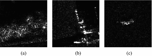

  

  ROIs. (a) natural clutter; (b) man-made clutter; (c) target

• Recognition stage: fetch detailed information from target chips.

Target discrimination is the second stage in SAR-ATR system, its performance has a great influence on the whole performance of the system [4, 5].

Feature based scheme is widely used in SAR target discrimination [6, 7], which consists of training stage and testing stage, as show in Fig. 2.

Fig. 2.

Discrimination scheme based on GA

1.1 Training Stage

Some images are used as training set, while others as testing set. At first, some features are extracted from training images, then Genetic Algorithm (GA) is used to select the optimal combination of these features (one-class quadratic discriminator is used to judge whether the feature subset is good or not), as show in Fig. 2(a).

1.2 Testing Stage

As show in Fig. 2(b), corresponding optimal feature set we obtained at training stage are extracted from testing images, then one-class quadratic discriminator (OCQD) is used to discriminate targets from clutters.

2 Extraction of Features

Seven features including three pixel level features: area feature, peak power ratio feature and fractal dimension feature, and four spatial edge property features, are extracted to distinguish targets from clutters.

2.1 Area Feature $\left( {\varvec{f}_{1} = \varvec{A}} \right)$

Compute the threshold by using CFAR algorithm, area feature A is the number of pixels above this threshold.

2.2 PPR Feature $\left( {\varvec{f}_{2} = \varvec{PPR}} \right)$

Peak power ratio (PPR) is the ratio of a% brightest pixels’ power of the image to the total power of the image.

2.3 Fractal Dimension Feature $\left( {\varvec{f}_{3} = \varvec{FD}} \right)$

Fractal dimension feature defined as [8]:

$$ FD = \frac{{log\,N_{1} - log\,N_{2} }}{{log\,d_{2} - log\,d_{1} }} $$

(1)

$N_{1}$ is the minimal number of 1 × 1 boxes that can cover the brightest pixels in the image, $N_{2}$ is the minimal number of 2 × 2 boxes that can cover the brightest pixels in the image. $d_{1}$ = 1 and $d_{2}$ = 2 represents the side length of box.

2.4 Spatial Edge Property Features $\left( {\varvec{f}_{{\mathbf{4}}} - \varvec{f}_{{\mathbf{7}}} } \right)$ [9]

Assume the N × M image I changes with a parameter t, then the image is I(t), the pixel strength is $I_{ij}$(t). Do logarithmic operation on image I, every pixel deducts the mid-value of the image $\bar{I}$ to get standard image, denoted as:

$$ x_{ij} = I_{ij} - \bar{I} $$

(2)

Using sigmoidal function below to shift standard images:

$$ s\left( {\varvec{x};t} \right) = \frac{1}{{1 + exp\left( { - c\left( {\varvec{x} - t} \right)} \right)}}, - \infty < t < + \infty $$

(3)

In the expression, $c$ is a positive real number.

Then we get a bunch of new images w(t), each value of pixel in w(t) expresses as:

$$ w_{ij} \left( t \right) = s\left( {\varvec{x}_{ij} ;t} \right) $$

(4)

A measurement on dispersion degree of image pixel quality to image centroid is:

$$ r\left( t \right) = \frac{{\mathop \sum \nolimits_{i = 1}^{N} \mathop \sum \nolimits_{j = 1}^{M} w_{ij} \left( t \right)\sqrt {\left( {i - i_{c} \left( t \right)} \right)^{2} + \left( {j - j_{c} \left( t \right)} \right)^{2} } }}{{\mathop \sum \nolimits_{i = 1}^{N} \mathop \sum \nolimits_{j = 1}^{M} w_{ij} \left( t \right)}} $$

(5)

In this formula, $i_{c}$ and $j_{c}$ are center-of-mass coordinates of images.

Obtain the best threshold $t_{0}$ when r(t) changes the most:

$$ t_{0} = argmax\left\{ { \left| {r^{\prime}\left( t \right)} \right| } \right\} $$

(6)

As ${\text{t}}_{0}$ is obtained, four spatial edge property features can be calculated as:

The average value of pixel mass in the image:

$$ f_{4} = log\frac{{\mathop \sum \nolimits_{i = 1}^{N} \mathop \sum \nolimits_{j = 1}^{M} w_{ij} \left( {t_{0} } \right)}}{MN} $$

(7)

The spatial scatter extension feature of pixels:

$$ f_{5} = r\left( {t_{0} } \right) $$

(8)

Inflexion point:

$$ f_{6} = r^{\prime}\left( {t_{0} } \right) $$

(9)

Acceleration:

$$ f_{7} = r^{\prime\prime\prime}\left( {t_{0} } \right) $$

(10)

3 Improved Feature Selection Method Based on GA

GA is an intelligent algorithm that can search best combination of features, it is widely used in object detection [8, 10,11,12].

As show in Fig. 3, feature selection based on GA mainly contains five problems: chromosome encoding; initialization of population; design of fitness function; selection of genetic operators; Updating population.

Fig. 3.

Feature selection based on genetic algorithm

3.1 Chromosome Encoding

A chromosome contains seven binary genes, stands for seven corresponding features, if a gene is 1, then corresponding feature is selected, otherwise, the feature is not selected. Figure 4 is an example of how a chromosome is encoded.

Fig. 4.

Feature subsequence

3.2 Initializing Population

To ensure the diversity of genes, we randomly generate 100 chromosomes as initial population.

3.3 Design of Fitness Function

Every chromosome has a fitness value calculated by fitness function, the function should reveal our purpose, which is the combination of selected features has lowest classification error rate and computation complexity. We define fitness function as:

$$ F\left( f \right) = - (k\,log_{10} \left( l \right) + n_{f} log_{10} (n_{c} ) - q *d_{max} ) $$

(11)

In the function, k is the number of selected features, l is the number of candidate features; $n_{f}$ is the number of classification errors that classify clutters into target class, we use OCQD to compute $n_{f}$, $n_{c}$ is the number of clutters in clutter class; $d_{max}$ is the maximum distance between targets and target class, q is a positive real number, we set q as 0.03 in our experiment.

3.4 Genetic Operators Selection

We choose three algorithms to search the best individual in population. Selection algorithm find top 20 individuals (unselected individuals set ones) and deliver them to the cross algorithm; set cross rate as 0.8, when it occurs, adjacent individuals change their genes randomly; set initial mutation rate as 0.01, the rate increases by 0.02 as fitness value of best individual does not improve, when mutation occurs, choose and reverse a gene in the individual randomly.

3.5 Updating Population

We update the population after three operators if the largest fitness value of new population is larger than the largest fitness value of the old population, repeating the loop until the mutation rate is higher than 0.09. Then we obtain selected features, as well as mean vector, covariance matrix and $d_{max}$ of training target class.

4 One Class Quadratic Discriminator

Unlike Bayes discriminator [8, 10], we only describe the similarity degree of a ROI to target class, when the degree is under a specific threshold, the ROI is considered as a target, otherwise as a clutter. Let the target class be $C_{1}$, clutter class be $C_{2}$, and the feature subsequence obtained by training data of $C_{i}$ (i = 1, 2) be $f_{i1}$, $f_{i2} , \ldots ,f_{{iM_{T} }}$ ($M_{T}$ is the number of training images of $C_{i}$). The mean and covariance matrix of target class $C_{1}$ can be calculated as following:

$$ \varvec{\mu}_{1} = \frac{1}{{M_{T} }}\sum\nolimits_{j = 1}^{{M_{T} }} {\varvec{f}_{1j} } $$

(12)

$$ \varvec{\varSigma}_{1} = \frac{1}{{M_{T} }}\sum\nolimits_{j = 1}^{{M_{T} }} {\left( {\varvec{f}_{1j} -\varvec{\mu}_{1} } \right)\left( {\varvec{f}_{1j} -\varvec{\mu}_{1} } \right)^{T} } $$

(13)

Let the extracted feature vector of a training image be ${\mathbf{f}}$. The quadratic distance of ${\mathbf{f}}$ to class $C_{1}$ is:

$$ d_{i} = \left( {{\mathbf{f}} -\varvec{\mu}_{1} } \right)^{T}\varvec{\varSigma}_{1}^{ - 1} \left( {{\mathbf{f}} -\varvec{\mu}_{1} } \right) $$

(14)

4.1 Application of OCQD in Training Stage

Firstly, computing $d_{1}$ which is the quadratic distance that target image to $C_{1}$, set the maximal $d_{1}$ as $d_{max}$, secondly, we calculate quadratic distance $d_{2}$ that clutter image to $C_{1}$, $n_{f}$ is the number of clutter images that quadratic distance less than $d_{max}$, which can express as:

$$ n_{f} = |\{ i|d_{2} < d_{max} ,1 \le i \le m\} | $$

(15)

Where m is the number of clutter images in training database. According to Eq. (11), fitness value of particular feature subsequence can be obtained.

4.2 Application of OCQD in Testing Stage

Mean vector, covariance matrix and $d_{max}$ of class $C_{1}$ corresponding to optimal feature subsequence can be obtained at training stage, quadratic distance of every testing image to class $C_{1}$ can be easily calculated, we consider an image whose quadratic distance smaller than $d_{max}$ as target, while larger than $d_{max}$ as clutter.

5 Experiments

5.1 Introduction of MSTAR Database

Resolution of MSTAR database is 0.3 × 0.3 m, HH polarization mode, X-band, under 15 degree depression angle and the distance is about 5 km. Target class contains 8 kind of vehicles, including 2S1, T62, T72, ZSU tanks; BRDM2, BTR60, ZIL armored vehicles; D7 bulldozer. Each type of target distributed in the entire 360 degree azimuth coverage, and image size is 128 × 128 pixels, we choose 75 targets covering 360 degree azimuth from each type of target class (total target number is 600), randomly choosing 200 target chips as training data and 400 chips as testing data. Clutter class contains 100 clutters, the total clutter coverage is about 10 ${\text{km}}^{2}$, including rural areas and urban areas, using CFAR detector based on Rayleigh distribution [13, 14], set false alarm rate as 0.001, we obtain 789 clutter chips in the size of 128 × 128 pixels, randomly choosing 292 chips as training data and 497 chips as testing data.

5.2 Experiment Results

Experiment Condition

Experiment condition is Core2 CPU, 2G memory, with the use of Matlab7.10.0. The average time of extracting all features is less than 0.5 s for a 128 × 128 image.

Feature Selection Based on GA

At training stage, we extract seven features for each training chips, run GA 10 times by using new method and traditional method [8, 10], respectively. As show in Tables 1 and 2, we obtain the best combination of seven features. The average efficiency of feature selection based on GA is improved by 77%.

Table 1. Feature selection based on GA using bayes discriminator

Table 2. Feature selection based on GA using OCQD discriminator

Quadratic Distance Distribution Graphs

As optimal feature subsequence is obtained, OCQD is used to calculate the quadratic distance of each image to class $C_{1}$, to see classification result clearly, define new quadratic distance as Eq. (16), distribution of $d_{new}$ is shown in Fig. 5. In distribution graphs, targets above 0-axis and clutters below 0-axis are considered as correct classification.

Fig. 5.

Quadratic distance distribution

$$ d_{new} = d_{max} - d_{i} $$

(16)

As show in Fig. 5, (a) is optimal subsequence used on training database, all images are classified correctly; (b) is optimal subsequence used on testing database, all targets are classified correctly, while 4 clutters are classified incorrectly; (c) is seven features used on training database, all images are classified correctly; (d) is seven features used on testing database, 1 target and 2 clutters are classified incorrectly.

From the distribution graphs we can see, the proposed method have a good performance on feature selection and target discrimination (target classification correction is more important than clutter classification correction).

Comparison of Discrimination Performance

At testing stage, optimal subsequence of features is extracted. Comparison with traditional method [8, 10] and proposed method on discrimination rate (DR) (DR means the rate that classify images to the right class) is showed in Fig. 6. From the bar graph we can see:

Fig. 6.

Discrimination rate (Our Method vs. Old Method)

• 1. Using optimal feature subsequence selected by GA either by new method or by traditional method to discriminate, we can achieve higher target discrimination rate than using all seven features.

• 2. Compared to traditional method, our method has higher target DR (100% to 99.5% on training data, 100% to 98.5% on testing data) and total DR (100% to 99.78% on training data, 99.55% to 99% on testing data).

• 3. Proposed method has lower clutter DR on testing data (99.4% to 99.2%).

Visualized Discrimination Result

As the imagery of clutter images and targets are under the same condition, we choose 8 types of targets randomly and embed them into clutter images, smooth edge of targets and clutter image, set false alarm rate as 0.001, CFAR detector based on Rayleigh distribution [13, 14] is used to achieve chips of target and clutter. Discrimination performance of proposed method and old method are similar until clutter-like target is chosen. As show in Fig. 7, (a) is embedded SAR image; (b) is the result of CFAR detector, 8 target chips and 29 clutter chips are obtained (object in red rectangle is target, object in green rectangle is clutter); (c) is the discrimination result of old method, 7 targets are correct classified, 1 target is not detected, all of clutters are classified correctly; (d) is the discrimination result of proposed method, as we can see, 8 targets are classified correctly, while 2 clutters are classified incorrectly.

Fig. 7.

Target discrimination results on embedded SAR images (Color figure online)

6 Conclusion

In this paper, an improved method on feature selection based on GA is proposed, one-class quadratic discriminator (OCQD) is used in this method. By using limited number of regular features, we can achieve better performance than traditional methods. Our experiment is based on MSTAR database. At first, 600 target chips and 789 clutter chips in the size of 128 × 128 pixels are obtained by using CFAR detector, then 200 target chips and 292 clutter chips are chosen as training data randomly, the rest as testing data. Compared to traditional methods [8, 10], our method has higher target discrimination rate (100% to 99.5% and 100% to 98.5% on training data and testing data, respectively), target discrimination experiment on embedded SAR images also show this characteristic, meanwhile, proposed method improves efficiency of feature selection based on GA by about 77%. But new method shows slight inadequate capacity of clutter discrimination (99.4% by old method and 99.2% by proposed method on testing data). Considering that cost brought about by target classification error is more serious than that brought about by clutter classification error, our new method has better performance than traditional methods on target discrimination.

References

Dudgeon, D.E., Lacoss, R.T.: An overview of automatic target recognition. Linc. Lab. J. 6(1), 3–10 (1993)
Bhanu, B., Dudgeon, D.E., Zelnio, E.G., Rosenfeld, A., Casasent, D., Reed, I.S.: Guest editorial introduction to the special issue on automatic target detection and recognition. IEEE Trans. Image Process. 6(1), 1–6 (1997)
Oliver, C.J., Quegan, S.: Understanding Synthetic Aperture Radar Images. Artech House, Boston (1998)
Novak, L.M., Owirka, G.J., Brower, W.S., Weaver, A.L.: The automatic target-recognition system in SAIP. Linc. Lab. J. 10(2), 187–202 (1997)
Kreithen, D.E., Novak, L.M.: Discriminating targets from clutter. Linc. Lab. J. 6(1), 25–51 (1993)
Blacknell, D.: Adaptive design and characterisation of features for SAR ATR. In: Proceedings of the SPIE Conference on Algorithms SAR Imagery IV, vol. 4382, pp. 252–263 (2001)
Krawiec, K., Bhanu, B.: Visual learning by coevolutionary feature synthesis. IEEE Trans. Syst. Man Cybern. B Cybern. 35(3), 409–425 (2005)
Bhanu, B., Lin, Y.: Genetic algorithm based feature selection for target detection in SAR images. Image Vis. Comput. 21, 591–608 (2003)
Verbout, S.M., Novak, L.M.: New image features for discriminating targets from clutter. In: Proceedings of SPIE Conference on Algorithms SAR Imagery IV, vol. 3395, pp. 120–137 (1998)
Gao, G.: An improved scheme for target discrimination in high-resolution SAR images. IEEE Trans. Geosci. Remote Sens. 49(1), 277–294 (2011)
Lin, Y., Bhanu, B.: Evolutionary feature synthesis for object recognition. IEEE Trans. Syst. Man Cybern. C: Appl. Rev. 35(2), 156–171 (2005)
Bhanu, B., Lin, Y.: Object detection in multi-modal images using genetic programming. Appl. Soft Comput. 4(2), 175–201 (2004)
Gao, G., Kuang, G., Zhang, Q., Li, D.: Fast detecting and locating groups of targets in high-resolution SAR images. Pattern Recogn. 40(4), 1378–1384 (2007)
Greco, M.S., Gini, F.: Statistical analysis of high-resolution SAR ground clutter data. IEEE Trans. Geosci. Remote Sens. 45(3), 566–575 (2007)
Author information
Authors and Affiliations
Corresponding author
Editor information
Editors and Affiliations
Rights and permissions
Copyright information
© 2017 Springer International Publishing AG
About this paper
Cite this paper
Li, Y., Cai, A. (2017). An Improved Feature Selection Method for Target Discrimination in SAR Images. In: Zhao, Y., Kong, X., Taubman, D. (eds) Image and Graphics. ICIG 2017. Lecture Notes in Computer Science(), vol 10668. Springer, Cham. https://doi.org/10.1007/978-3-319-71598-8_56
Download citation
DOI: https://doi.org/10.1007/978-3-319-71598-8_56
Published:
Publisher Name: Springer, Cham
Print ISBN: 978-3-319-71597-1
Online ISBN: 978-3-319-71598-8
eBook Packages: Computer ScienceComputer Science (R0)