An Efficient and Robust Visual Tracking via Color-Based Context Prior Model

Abstract

Real-time object tracking has been widely applied to time-critical multimedia fields such as surveillance and human-computer interaction. It is a challenge to balance accuracy and speed in tracking. Spatio-Temporal Context tracker (STC) formulates the spatio-temporal relationship between the object and its surrounding background, and achieves good performance in accuracy and speed. However, the context prior model only utilizes the grayscale feature which is not efficient. When the target is not obvious in the context, or the context exists a similar interference compared to the target, STC tracker drifts from the target. To solve the problem, we exploit the standard color histograms of the context to build a discriminative context prior model. More specifically, we utilize an effective lookup-table to compute the prior context model at a low computational cost. Finally, extensive experiments on challenging sequences show the effectiveness and robustness of our proposed method.

1 Introduction

Visual Object Tracking is a hot topic in the field of computer vision. Based on image sequences, visual object tracking has been widely applied to intelligent robots, monitoring, factory automation, man-machine interface, vehicle tracking to name a few. However, there is still a challenge in visual tracking for many factors such as illumination variation, deformation, occlusion, scale variation and fast motion, etc.

Generally visual object tracking is divided into two categories: generative model methods and discriminative model methods. Generative models [1, 2] learn a representative appearance model to identify the target, and search the best-matching windows. On the other hand, discriminative models [3, 4] focus on training a classifier which aims at distinguishing the target and the background. The biggest difference of generative and discriminative models is that discriminative models use the background information. Background information is advantageous for effective tracking [5, 6], thus the discriminative methods are generally better than the generative methods. However, the discriminative methods have some shortcomings, such as lack of samples. Besides, speed is a very important metric in practical application. Trackers that run at a low speed with expensive computing cost have no practical value. Therefore, study on fast and robust tracking methods is valuable.

Correlation filter (CF) based trackers have got much attention for their good performance both in speed and accuracy. CF based trackers use a learned filter to localize the target in the next frame by confirming the position of maximal response. Spatio-Temporal Context (STC) [7] tracker follows a similar workflow as CF based trackers. There exists a strong spatio-temporal relationship between the scenes containing the object in consecutive frames. STC exploits the context information, and performs favorably in IV or OCC scenarios. But when the target is not obvious in the context, or the context exist a similar interference compared to the target, STC has drifting problem for its prior model only use the grayscale features. In this paper, we utilize the color histograms to get the saliency object likelihood scores in a context tracking framework, and take it as the context prior model, as shown in Fig. 1. The object region is more significant in proposed prior model compared with the STC prior model. Our model is well applied to time-critical applications for the favorable simplicity of our representation.

Fig. 1.

The proposed prior model using color histogram to distinguish object from background. (a) is the original context image. (b) is the STC prior model. (c) is the proposed saliency prior model. (Color figure online)

Our contributions are as follows: we propose a discriminative context prior model to distinguish the object region from the background. It relies on standard color histograms and achieves good performance on a variety of challenging sequences. More specifically, we utilize an effective lookup-table to compute the context prior model over a large search region at a low computational cost. Finally, we extensively evaluate our method on benchmark datasets to prove its good performance compared with other state-of-the-art trackers.

The rest of this paper is organized as follows: First, we introduce the related work in Sect. 2. Then our tracking method is described in Sect. 3. Extensive experiments are conducted to evaluate the proposed method compared with other state-of the-art methods in Sect. 4. Section 5 concludes the paper.

2 Related Work

In this section, we provide a brief overview of trackers, and discuss the methods closely related to our proposed method (CF based trackers).

Generative trackers describe the target with an appearance model. They search the best matched region by the updated generative model. Examples of this category include mean shift tracker [8], incremental tracker (IVT) [9], multi-task tracker (MTT) [2], and object tracker via structured learning [10] to name a few. Discriminative trackers treat the object tracking as a classification problem. They use a classifier to predict the foreground and background. Examples of this category include multiple instance learning (MIL) [11], correlation filter (CF) based trackers and so on.

CF based trackers design correction filters to produce correction peak for the tracking target, but generating low response to the background. Correction filters only use a small part of the computational power. They adapt the product of FFT domain to replace the convolution of spatial domain, and achieve hundreds of frame per second. The proposal of Minimum Output Sum of Squared Error (MOSSE) [12] makes the correction filters appropriate for online tracking. Many improvements have been made based on the framework of MOSSE. Henriques et al. [13] proposed using correction filter in a kernel space based on exploiting the circulant structure of tracking-by-detection with kernels (CSK). CSK uses a dense sampling strategy, which can extract all information of the target. Although CSK has made gratifying achievements in terms of speed, the grayscale feature is insufficient in the description of the target appearance. KCF [14] is proposed to improve the performance of CSK by using of HOG features. By further handling the scale changes, SAMF [15] is proposed and achieve good performance.

Context information has already been considered in many tracking methods. In general, they extract key points around the target and describe them with SURF, SIFT or other descriptors. But these methods may ignore the crucial information and spend much computational cost. Zhang et al. efficiently adapt the context information in filter learning and model the scale based on the correlation response. Robust feature representation plays important role in visual tracking [16]. While in STC, the tracker uses grayscale features, which lack of description of the appearance. Our saliency context prior model makes full use of color information to make the target saliency from the background. Besides, to reduce the cost of computing, we utilize an effective lookup-table over a large search region at a low computational cost. The proposed prior model will be introduced below.

3 The Proposed Method

3.1 Dense Spatio-Temporal Context Prior Model

STC tracker can be treated as calculating the possibility that a target appears at a sampling area. It computes a confidence map which estimates the object location likelihood:

$$ {\text{c}}\left( {\mathbf{x}} \right) = P\left( {{\mathbf{x}} |o} \right) $$

(1)

where x is the object location and o denotes the object present in the scene. The maxing c(x) is the target location. Equation (1) can be expressed as

$$ {\text{c}}\left( {\mathbf{x}} \right) = \sum\nolimits_{{{\text{c}}\left( {\mathbf{z}} \right) \in {\text{X}}^{\text{c}} }} {P({\mathbf{x}},{\text{c}}\left( {\mathbf{z}} \right)|o) = \sum\nolimits_{{{\text{c}}\left( {\mathbf{z}} \right) \in {\text{X}}^{\text{c}} }} {P\left( {{\mathbf{x}} |{\mathbf{c}}\left( {\mathbf{z}} \right),o} \right)P({\mathbf{c}}\left( {\mathbf{z}} \right)|o)} } $$

(2)

In Eq. (2), c(z) means the feature set of the context. P(x|c(z), o) is the spatial context model, which means the relationship between the target and surrounding points in the context. P(c(z)|o) is the context prior model, which expresses the exterior feature of points in the context. STC tracker is to locate the target by designing the prior probability P(c(z)|o) and updating the spatial context model P(x|c(z), o).

The conditional probability function P(x|c(z), o) in Eq. (2) is described as

$$ P\left( {{\mathbf{x}} |{\mathbf{c}}\left( {\mathbf{z}} \right),o} \right) = h^{sc} \left( {{\mathbf{x}} - {\mathbf{z}}} \right) $$

(3)

where $h^{sc} \left( {{\mathbf{x}} - {\mathbf{z}}} \right)$ means the relative distance and direction between object location x and its local context location z, presenting the relationship between an object and its spatial context.

The context prior probability is

$$ P\left( {{\mathbf{c}}\left( {\mathbf{z}} \right) |o} \right) = I\left( \varvec{z} \right)\omega_{\sigma } \left( {{\mathbf{z}} - {\mathbf{x}}^{*} } \right) $$

(4)

where I( z ) is image grayscale, and $\omega_{\sigma } \left( {{\mathbf{z}} - {\mathbf{x}}^{*} } \right)$ is weighting function defined by

$$ \omega_{\sigma } \left( \varvec{z} \right) = ae^{{ - \frac{{\left| {\mathbf{x}} \right|^{2} }}{{\sigma^{2} }}}} $$

(5)

In Eq. (5), a is a normalization constant restricts P(c(z)|o) to range from 0 to 1. $\sigma$ is a scale parameter.

3.2 The Proposed Saliency Prior Model

STC tracker utilizes the grayscale features. When the target is not obvious in the context, or the context exist a similar interference compared to the target, STC has the tracking drift problem. To distinguish object region from background, we employ a color histogram on the current image I with Bayesian classifier. Let $b_{{\mathbf{x}}}$ denotes the bin b assigned to the color components of ${\text{context}}$. For an object region O and its surrounding region S, we get the object likelihood as:

$$ P\left( {{\mathbf{x}} \in O |O,S,b_{{\mathbf{x}}} } \right) = \frac{{P\left( {b_{{\mathbf{x}}} |{\mathbf{x}} \in O} \right){\text{P}}\left( {{\mathbf{x}} \in O} \right)}}{{P\left( {b_{{\mathbf{x}}} |{\mathbf{x}} \in S} \right){\text{P}}\left( {{\mathbf{x}} \in S} \right)}} $$

(6)

Let $H_{\varOmega }^{I} \left( {b_{{\mathbf{x}}} } \right)$ means the b-th bin of the non-normalized histogram H of region $\varOmega$. We estimate the likelihood with the color histogram. i.e. $P\left( {b_{{\mathbf{x}}} |{\mathbf{x}} \in O} \right) \approx \frac{{H_{O}^{I} \left( {b_{{\mathbf{x}}} } \right)}}{\left| O \right|}$ and $P\left( {b_{x} |{\mathbf{x}} \in S} \right) \approx \frac{{H_{S}^{I} \left( {b_{{\mathbf{x}}} } \right)}}{\left| S \right|}$. The $\left| \cdot \right|$ means the number of pixels of a region. Furthermore, the prior probability can be estimated as $P\left( {b_{{\mathbf{x}}} |{\mathbf{x}} \in O} \right) \approx \frac{\left| O \right|}{\left| S \right|}$. Then Eq. (6) can be simplified to

$$ P\left( {{\mathbf{x}} \in O |O,S,b_{{\mathbf{x}}} } \right) = \left\{ {\begin{array}{*{20}c} {\frac{{H_{O}^{I} \left( {b_{{\mathbf{x}}} } \right)}}{{H_{S}^{I} \left( {b_{{\mathbf{x}}} } \right)}}} & {I\left( x \right) \in S} \\ {0.5} & { {\text{otherwise}} } \\ \end{array} } \right. $$

(7)

This discriminative model allows us to distinguish object and background pixels. In Eq. (7), the object likelihood scores can be computed via an efficient lookup-table, which can greatly reduce the computational cost. We updated the object model on a regular basis using the linear interpolation:

$$ P_{1:t} \left( {{\mathbf{x}} \in O |b_{{\mathbf{x}}} } \right) = \eta {\text{P}}\left( {{\mathbf{x}} \in O |b_{{\mathbf{x}}} } \right) + \left( {1 - \eta } \right){\text{P}}_{1:t - 1} \left( {{\mathbf{x}} \in O |b_{{\mathbf{x}}} } \right) $$

(8)

where $\eta$ means the learning rate.

In our method, the object model ${\text{P}}\left( {{\mathbf{x}} \in O |O,S,b_{{\mathbf{x}}} } \right)$ is treated as the context prior probability. As with Eq. (4), then the context prior probability becomes

$$ P\left( {\varvec{c}\left( {\mathbf{x}} \right) |O} \right) = {\text{P}}\left( {{\mathbf{x}} \in O |O,S,b_{{\mathbf{x}}} } \right)\upomega_{\upsigma} \left( {{\mathbf{x}} - {\mathbf{x}}^{*} } \right) $$

(9)

As the framework of STC, The confidence map is

$$ {\mathbf{c}}\left( {\mathbf{x}} \right) = {\text{P}}\left( {{\mathbf{x}} |O} \right) = b{\text{e}}^{{ - |\frac{{{\mathbf{x}} - {\mathbf{x}}^{*} }}{\alpha }|^{\beta } }} $$

(10)

where b is a normalization constant, $\alpha$ is a scale parameter and $\beta$ is a shape parameter.

Associate Eqs. (3) and (9), the confidence map is

$$ {\mathbf{c}}_{{{\mathbf{t + 1}}}} \left( {\mathbf{x}} \right) = F^{ - 1} \left( { F\left( {H_{t + 1}^{stc} \left( {\mathbf{x}} \right)} \right) \odot F\left( { P_{t + 1} \left( x \right)\omega_{{\sigma_{t} }} \left( {{\mathbf{x}} - {\mathbf{x}}_{{\mathbf{t}}}^{*} } \right)} \right)} \right) $$

(11)

Therefore, the spatial context model is

$$ h^{sc} \left( {\mathbf{x}} \right) = F^{ - 1} \left( {\frac{{F\left( {be^{{ - |\frac{{{\mathbf{x}} - {\mathbf{x}}^{*} }}{\alpha }|^{\beta } }} } \right)}}{{F\left( { P\left( {\mathbf{x}} \right)\omega_{\sigma } \left( {{\mathbf{x}} - {\mathbf{x}}^{*} } \right)} \right)}}} \right) $$

(12)

The object location ${\mathbf{x}}_{{{\mathbf{t}}{\mathbf{ + 1}}}}^{{\mathbf{ * }}}$ in the (t + 1)-th frame is determined by maximizing the new confidence map

$$ {\mathbf{x}}_{{{\mathbf{t + 1}}}}^{{\mathbf{*}}} = {\text{arg}}\max_{{{\mathbf{x}} \in\Omega _{\text{c}} \left( {{\mathbf{x}}_{{\mathbf{t}}}^{*} } \right)}} {\mathbf{c}}_{{{\mathbf{t}}{\mathbf{ + 1}}}} \left( {\mathbf{x}} \right) $$

(13)

The spatio-temporal context model id undated by

$$ H_{t + 1}^{stc} = \left( {1 - \rho } \right)H_{t}^{stc} + \rho h_{t}^{sc} $$

(14)

where $\rho$ denotes learning parameter and $h_{t}^{sc}$ is the spatial context computed by Eq. (12) at the t-th frame.

3.3 Lookup-Table Update Scheme

To reduce the amount of computational cost, we adapt a lookup-table to calculate the object likelihood score. Here we will introduce how to get the lookup-table from a context and its update scheme.

For a given context, there exist three color components. Each component ranges from 0 to 255. We can get the index of the component of each pixel. The index ranges from 1 to $256^{3}$. So it will cost a large computational cost to get the color histogram. To reduce the computational cost, we divide the pixel from 256 to 16 levels. The index range will be reduced from $256^{3}$ to $16^{3}$. Then the histogram of object region $H_{O}^{I} \left( {\varvec{b}_{{\mathbf{x}}} } \right)$ and the histogram of surrounding background region $H_{S}^{I} \left( {\varvec{b}_{{\mathbf{x}}} } \right)$ can be calculated. We can get the object likelihood $P\left( {{\mathbf{x}} \in O |O,S,b_{x} } \right)$ according to Eq. (7). The lookup-table is updated by Eq. (8).

For grayscale sequences, the computational cost is not as large as color sequences, and to better distinguish the object and background, we compute the histogram on 256 grayscale levels directly.

3.4 Scale Update Scheme

As with STC, The scale parameter is updated with the maximum of confidence map. The scale update scheme as

$$ \left\{ {\begin{array}{*{20}c} {s_{t}^{'} = \sqrt {\frac{{c_{t} \left( {x_{t}^{*} } \right)}}{{c_{t - 1} \left( {x_{t - 1}^{*} } \right)}}} } \\ {\overline{{s_{t} }} = \frac{1}{n}\sum\nolimits_{i = 1}^{n} {s_{t - i}^{'} } } \\ {s_{t + 1} = \left( {1 - \lambda } \right)s_{t} + \lambda \overline{{s_{t} }} } \\ {\sigma_{t + 1} = s_{t} \sigma_{t} } \\ \end{array} } \right. $$

(15)

In Eq. (15), ${\mathbf{c}}_{{\mathbf{t}}} \left( {{\mathbf{x}}_{{\mathbf{t}}}^{{\mathbf{*}}} } \right)$ is the confidence map and $s_{t}^{'}$ is the estimated scale between two consecutive frames. The estimated target scale $s_{t + 1}$ is obtained through filtering in which $\overline{{s_{t} }}$ is the average of estimated scales from n consecutive frames, and $\lambda$ is a fixed filter parameter.

The procedure of our algorithm is shown in Algorithm 1.

4 Experimental Results and Analysis

In this section, we evaluate the performance of proposed tracker on 17 challenging sequences provided on Online Test Benchmark [5]. The challenges involve 10 common attributes: illumination variation, out-of-plane rotation, scale variation, occlusion, deformation, motion blur, fast motion, in-plane-rotation, background clutter and low resolution.

The proposed tracker is compared with 11 state-of-the-art tracking methods in recent years. They are sparse collaborative appearance (SCM), the structured output tracker (Struck), tracking learning detection (TLD), CSK tracker, KCF tracker, STC tracker, deep learning tracker (DLT), Multi-Instance Learning (MIL), L1 tracker (L1APG), adaptive structural local sparse appearance model (ASLA) and Compressive Tracker (CT).

4.1 Experimental Setup

The proposed tracker is implemented in Matlab R2015a and runs at 137 frames per second results on Intel i5 2.5 GHz CPU, 4G RAM, Win7 system. We test 17 sequences on total 4200 frames. And the proceeding speed is 137 frames per second. The state of the target in the first frame is given by the ground truth. The parameter $\sigma_{t}$ in Eq. (12) is set to $\sigma_{1} = \frac{{h_{0} + w_{0} }}{2}$, where $h_{0} \;{\text{and}} \;w_{0}$ are height and width of the initial tracking rectangle. The scale parameter $s_{t}$ is set to $s_{1} = 1.$ The number of frames $n$ for updating scale in Eq. (15) is set to 5. The parameter $\lambda$ in Eq. (15) is set to 0.25. The parameter $\alpha$ is set to 2.25 and $\beta$ is set to 1. The learning parameter $\rho$ in Eq. (11) is set to 0.025. The learning rate of object model $\eta$ in Eq. (15) is set to 0.03. All the parameters are fixed for all experiments.

4.2 Evaluation Metrics

For quantitative evaluations, we use the center location error (CLE), the success plot and the precision plot. The CLE metric is defined as:

$$ {\text{CLE}} = \frac{1}{\text{N}}\sum\nolimits_{{{\text{i}} = 1}}^{\text{N}} {\sqrt {\left| {x_{t}^{i} - x_{g}^{i} } \right|^{2} + \left| {y_{t}^{i} - y_{g}^{i} } \right|^{2} } } $$

(16)

The success plot is based on the overlap ratio. The success plot is defined as ${\text{S}} = \frac{{area\left( {R_{t} \cap R_{g} } \right)}}{{area\left( {R_{t} \cup R_{g} } \right)}}$, where $R_{t}$ is a tracked bounding box and $R_{g}$ is the ground truth bounding box, and the result of one frame is considered as a success if ${\text{S}} > 0.5$. The area under curve (AUC) of each success plot serves as the second measure to rank the tracking algorithms. Meanwhile, the precision plot illustrates the percentage of frames whose tracked locations are within the given threshold distance to the ground truth. A representative precision score with the threshold equal to 20 is used to rank the trackers.

4.3 Quantitative Comparisons

• (1) Overall Performance: Fig. 2 shows the overall performance of the 12 tracking algorithm in terms of success and precision plots. Note that all the plots are generated using the code library from the benchmark evaluation and the results of KCF are provided by the authors. In the success plot, the proposed algorithm achieve the AUC of 0.580, ranking second in the 12 trackers, which outperforms the STC method by 15.6%. Meanwhile, in the precision plot, the precision score of the proposed method is ranking first in the 12 trackers, and outperforms the STC method by18.6%.

  Fig. 2.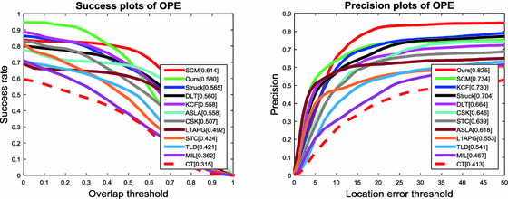

  

  The success plot and precision plot of OPE for 12 trackers. The performance score of success plot is the AUC value. The performance score of precision plot is at error threshold of 20 pixels.

Table 1 shows the CLE of the 17 sequences. In general our proposed method is ranking first and KCF is ranking second among 12 trackers, and ranking second both in the success rate and overlap rate, as shown in Table 2 and Table 3.

Table 1. Center location error (in pixels). The red fonts indicate the best performance. The green fonts indicate the second performance.

Table 2. Scores of success rate. The result of one frame is considered as a success if ${\text{S}} > 0.5$. The red fonts indicate the best performance. The green fonts indicate the second performance.

Table 3. Scores of overlap rate. The red fonts indicate the best performance. The green fonts indicate the second performance.

• (2) Attribute-based Performance: To analyze the strength and weakness of the proposed method, we evaluate the trackers on sequences with 10 attributes. We focus on 5 of 10 attributes. Figure 3 shows the success plots of views with 5 attributes and Fig. 4 shows the corresponding precision plots. In the following, we analyze the results based on scores of success plots which is more informative than the score at one position in the precision plot.

  Fig. 3.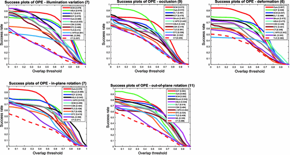

  

  The success plots of videos with 5 attributes. The number in the title indicates the number of sequences. Best viewed on color display.

  Fig. 4.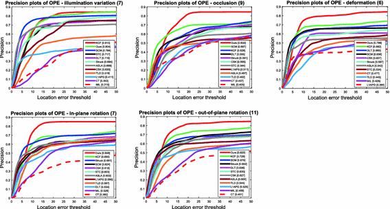

  

  The precision plots of videos with 5 attributes. The number in the title indicates the number of sequences. Best viewed on color display.

For the sequences with the deformation and in-plane rotation, the proposed algorithm ranks first among all evaluated trackers. The object color doesn’t change with deformation or rotation. So the proposed model can distinguishes object region from surrounding background, which make the tracking stable and drifting problem is avoided.

With the sequences with attributes of out-of-plane rotation and occlusion, the proposed algorithm ranks second among the evaluated methods with a narrow margin (less than 1%) to the best performing methods, corresponding to KCF and SCM respectively. The KCF method utilizes HOG features to describe the target and its local context region. SCM employ local features extracted from the local image patches, and utilize the target template from the first frame to handle the drift problem. Our method computes the object likelihood with the color histogram, and can track on the object whose color has little change.

For the videos with illumination variation, our method ranks fifth while SCM performs well. In illumination variation sequences, the color component of target changes, but the lookup-table is also corresponding to the target before illumination occurs. The object region may not be prominent in the proposed prior model.

In next section, we will illustrate the comparisons between the proposed method and other state-of-the-art method on the 17 sequences in Table 1.

4.4 Qualitative Comparisons

• (1) Deformation: Figure 5 shows some screenshots of the tracking results in three challenging sequences where the target objects undergo large shape deformation. In the Bolt sequence, the appearance of target and disturbance change due to shape deformation and fast motion. Only our method can track the target well. The CT, KCF, MIL, ASLA and L1APG methods undergo large drift at the beginning of the video (e.g. #10). The TLD method begins to drift at frame #80. After frame #150, only our method tracks the target well until to the end of the Bolt sequence. The target object in the Basketball sequence undergoes significant appearance variation duo to non-rigid body deformation. The TLD and Struck methods lose target at frame #30. L1APG and MIL algorithm lose track of target after frame #294. ALSA method begins to lose at frame #470. Only KCF, and our method perform well at all frames.

  Fig. 5.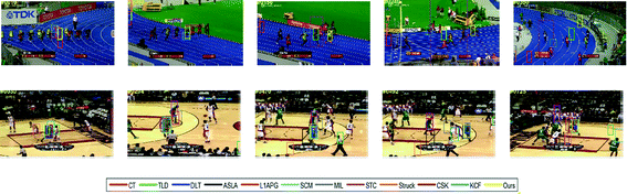

  

  Qualitative results of the 12 trackers over sequence Bolt and basketball, in which the targets undergo deformation. Best viewed on color display.

• (2) Illumination Variation: Figure 6 shows some sampled results in three sequences in which the target objects undergo large illumination changes. In the Car4 sequence, the moving car passes under a bridge and trees. Despite large illumination variation at frame #180, #200 and #240, the proposed method is able to track well. The CT, L1APG and MIL methods drift away from the target objects when sudden illumination variation occurs at frame #240. ALSA, DLT and SCM method handle scale variation well (e.g. #400, #500, #600). The object appearance in the Trellis sequence changes significantly due to variations in illumination and pose. Only KCF and our method perform well, and never lose from beginning to the end of sequence. CT, CSK, Struck and TLD methods lose the target during the tracking process, but when target moves close to their location, they keep up with the target again (e.g. #423, #569).

  Fig. 6.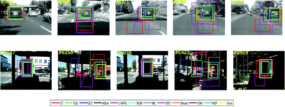

  

  Qualitative results of the 12 trackers over sequence Trellis and Car4, in which the targets undergo illumination variation. Best viewed on color display.

• (3) Heavy Occlusion: Figure 7 shows sampled results of three sequences where the targets undergo heavy occlusions. In the Football sequence, the target is almost fully occluded in the frame #292. Our method is able to locate on the target when it appears on the screen (# 362). In the FaceOcc1 sequence, the target is frequently occluded by a book (#237, #553, #745, and so on). STC, ASLA and MIL methods begin to fail track on the target on frame #237. TLD tracks on part of the target on frame #553. Struck, DLT, KCF and our method perform well in the entire sequence.

  Fig. 7.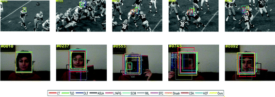

  

  Qualitative results of the 12 trackers over sequence Football and FaceOcc1, in which the targets undergo occlusion. Best viewed on color display.

• (4) In- Plane Rotation and Out-of-Plane Rotation: During the tracking process, rotation will result in shape deformation and visual changes. Figure 8 shows sampled results of sequences where the targets undergo both in-plane rotation and out-of plane rotation, the same as Bolt sequence in Fig. 4. The proposed method is always tracking on the object in the whole sequence.

  Fig. 8.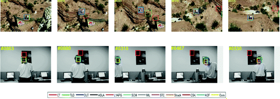

  

  Qualitative results of the 12 trackers over sequence MountainBike and David2, in which the targets undergo in- plane rotation and out-of-plane rotation. Best viewed on color display.

5 Conclusion

In this paper, we propose a robust object tracking approach based on color-based context prior model. We exploit the standard color histograms to distinguish the target from background, and build a discriminative context prior model. Our method refers to the STC tracking framework and scale update scheme. More specifically, to reduce the amount of calculation, we adapt an effective lookup-table, which can compute at a low computational cost. Moreover, numerous experiments are conducted to compare the proposed method with other relevant state-of-the-art trackers. Both quantitative and qualitative evaluations further demonstrate the effectiveness and robustness of the proposed method.

References

Sevilla-Lara, L., Learned-Miller, E.: Distribution fields for tracking. In: IEEE Conference on Computer Vision and Pattern Recognition, vol. 157, pp. 1910–1917. IEEE Computer Society (2012)
Ahuja, N., Liu, S., Ghanem, B., Zhang, T.: Robust visual tracking via multi-task sparse learning. In: Computer Vision and Pattern Recognition, vol. 157, pp. 2042–2049. IEEE (2012)
Hare, S., Saffari, A., Torr, P.H.S.: Struck: structured output tracking with kernels. In: IEEE International Conference on Computer Vision, vol. 23, pp. 263–270. IEEE (2012)
Wang, Q., Chen, F., Xu, W., Yang, M.H.: Object tracking with joint optimization of representation and classification. IEEE Trans. Circ. Syst. Video Technol. 25(4), 638–650 (2015)
Wu, Y., Lim, J., Yang, M.H.: Online object tracking: a benchmark. In: IEEE Conference on Computer Vision and Pattern Recognition, vol. 9, pp. 2411–2418. IEEE Computer Society (2013)
Wu, Y., Lim, J., Yang, M.H.: Object tracking benchmark. IEEE Trans. Pattern Anal. Mach. Intell. 37(9), 1834 (2015)
Zhang, K., Zhang, L.: Fast tracking via spatio-temporal context learning. Comput. Sci. (2013)
Comaniciu, D., Ramesh, V., Meer, P.: Kernel-based object tracking. IEEE Trans. Pattern Anal. Mach. Intell. 25(5), 564–575 (2003)
Cauwenberghs, G., Poggio, T.: Incremental and decremental support vector machine learning. In: Advances in Neural Information Processing Systems 13, vol. 1, pp. 409–415 (2001)
Zhang, T., Ghanem, B., Xu, C., Ahuja, N.: Object tracking by occlusion detection via structured sparse learning, vol. 71, no. 4, pp. 1033–1040 (2013)
Babenko, B., Yang, M. H., Belongie, S.: Visual tracking with online multiple instance learning. In: IEEE Conference on Computer Vision and Pattern Recognition, CVPR 2009, vol. 33, pp. 983–990. IEEE (2009)
Bolme, D.S., Beveridge, J.R., Draper, B.A., Lui, Y.M.: Visual object tracking using adaptive correlation filters. In: Computer Vision and Pattern Recognition, vol. 119, pp. 2544–2550. IEEE (2010)
Henriques, J.F., Caseiro, R., Martins, P., Batista, J.: Exploiting the circulant structure of tracking-by-detection with kernels. In: Fitzgibbon, A., Lazebnik, S., Perona, P., Sato, Y., Schmid, C. (eds.) ECCV 2012. LNCS, vol. 7575, pp. 702–715. Springer, Heidelberg (2012). https://doi.org/10.1007/978-3-642-33765-9_50
Henriques, J.F., Caseiro, R., Martins, P., Batista, J.: High-speed tracking with kernelized correlation filters. IEEE Trans. Pattern Anal. Mach. Intell. 37(3), 583–596 (2014)
Li, Y., Zhu, J.: A scale adaptive kernel correlation filter tracker with feature integration. In: Agapito, L., Bronstein, M., Rother, C. (eds.) ECCV 2014 Workshops. LNCS, vol. 8926, pp. 254–265. Springer, Cham (2015). https://doi.org/10.1007/978-3-319-16181-5_18
Han, Y., Deng, C., Zhang, Z., Li, J., Zhao, B.: Adaptive feature representation for visual tracking. arXiv preprint arXiv:1705.04442 (2017)
Acknowledgements
This work is supported by the Chang Jiang Scholars Programme (Grant No. T2012122), and 111 Project of China under Grant B14010.
Author information
Authors and Affiliations
Corresponding author
Editor information
Editors and Affiliations
Rights and permissions
Copyright information
© 2017 Springer International Publishing AG
About this paper
Cite this paper
Yu, C., Zhao, B., Zhang, Z., Li, M. (2017). An Efficient and Robust Visual Tracking via Color-Based Context Prior Model. In: Zhao, Y., Kong, X., Taubman, D. (eds) Image and Graphics. ICIG 2017. Lecture Notes in Computer Science(), vol 10666. Springer, Cham. https://doi.org/10.1007/978-3-319-71607-7_7
Download citation
DOI: https://doi.org/10.1007/978-3-319-71607-7_7
Published:
Publisher Name: Springer, Cham
Print ISBN: 978-3-319-71606-0
Online ISBN: 978-3-319-71607-7
eBook Packages: Computer ScienceComputer Science (R0)