
Abstract
Nowadays, Depth Learning with Convolution Neural Networks (CNN) has become a well known method in object recognition task to generate descriptions and classify learned features and gradually took over. There are few CNN applied studies on leaves recognition and classifier task that mainly use the existing CNN architecture and pre-trained models. This paper proposes a CNN model for leaves classifier based on thresholding leaf pre-processing extract vein shape data and augmenting training data with reflection and rotation of the image. Preprocessing to reduce the storage capacity of data and increases the computational efficiency of the model. This model was experimented on collector leaves data set in the Mekong Delta of Vietnam, the Flavia leaf data set and the Swedish leaf data set. The classification results indicate that the proposed CNN model is effective for leaf recognition with an accuracy greater than 95%.
1 Introduction
Image classification task is usually based on features engineering such as SIFT, HOG, SURF,… combined with a learning algorithm in these features engineering spaces such as SVM, Neuron, KNN… This leads to the efficiency of all approaches that depend heavily on predefined features. Image features engineering itself is a complex field, needed to be changed and revisited at hand for each problem or data set involved.
Today, with the development of neural networks, neural network architecture has been used as an effective solution to extract high level features from data. Deep Convolutional Neural Networks architectures can accurately portray highly abstract properties with condensed data, while preserving the most up-to-date characteristics of raw data. This is beneficial for classification or prediction. In recent times, CNN has emerged as an effective framework for describing features and identities in image processing. CNN can learn basic filters automatically and combine them hierarchically to describe underlying concepts to identify patterns. CNN does not need computation features engineering. It takes time and effort. The generalization of the method makes it a practical and scalable approach to the various application problems of classification and recognition.
In 2000, Oide and Ninomiya [1] used neural networks to classify soybean leaves using a Hopfield network and a simple perceptron. In 2001, Soderkvist [2] used leaf morphology to train back propagation neurons to classify 15 plants in Sweden. This data set used in the experiment and then become a standard data set - Swish data sets. Many later experiments used this data set. There are studies applying deep architecture to image recognition in advance. Krizhevsky et al. [3] has used Deep Convolutional Neural Networks for ImageNet and their research results have created a new rush for depth learning.
Several publications have suggested the use of CNN in leaf classification in recent years. Jassmann et al. [4] develops an application for classifying plants, based on leaf images. The system uses a CNN in a mobile application for mobile phones to categorize the nature of the leaf, trained with the ImageCLEF data set. The proposed architecture consists of a convoluted layer, followed by a composite layer and two fully connected layers applied to the 60 × 80 pixel input image. Wu et al. proposed a simplified version of AlexNet for leaf recognition [5]. They have used parametric linear units (PReLU) instead of ReLU. In [6] He et al. proposed a one-to-one connection, named Single Connector (SCL), added to the proposed CNN architecture to create some improvements. This method has been tested on the ICL leaf database and the results reflect an increase in accuracy.
Plant disease identification includes the processing of leaf recognition. Sladojevic et al. [7], have been interested in a new method for developing a disease-identification model based on leaf classification of images, using CNN. The developmental model was able to recognize 13 healthy plant leaf diseases, with the ability to discriminate leaves from the surrounding environment.
In this study, we approached leaf-based visual recognition based on the vein’s morphology using the depth learning model. Specifically, Convolutional Neural Network (CNN) is one of the advanced depth learning models that helps us build intelligent systems with high precision as present. Our model implemented is depicted in Fig. 1, the initial image is well-adapted to reduce the amount of unnecessary color information and clarify the vein characteristics then using depth learning neural network for classification.

Our scheme implementation
The rest of the paper is organized as follows. In Sect. 2: neural networks and CNN. In Sect. 3: CNN models for leaves recognition. In Sect. 4: experiments. In Sect. 5: conclusions.
2 Convolution Neural Network (CNN)
2.1 Artificial Neural Networks
Neural networks are inspired by biological neural systems. The basic computational unit of the brain is a neuron and they are connected with synapses.
In the neural network computational model, the signals that travel along the axons (e.g., ×0) interact multiplicatively (e.g., w0 × 0) with the dendrites of the other neuron based on the synaptic strength at that synapse (e.g., w0). Synaptic weights are learnable and control the influence of one neuron or another. The dendrites carry the signal to the cell body, where they all are summed. If the final sum is above a specified threshold, the neuron fires, sending a spike along its axon. In the computational model, it is assumed that the precise timings of the firing do not matter and only the frequency of the firing communicates information. Based on the rate code interpretation, the firing rate of the neuron is modeled with an activation function f that represents the frequency of the spikes along the axon. A common choice of activation function is sigmoid. In summary, each neuron calculates the dot product of inputs and weights, adds the bias, and applies non-linearity as a trigger function (for example, following a sigmoid response function).
A CNN is a special case of the neural network described above. A CNN consists of one or more convolutional layers, often with a subsampling layer, which are followed by one or more fully connected layers as in a standard neural network.
A neural network is a system of interconnected artificial “neurons” that exchange messages between each other. The connections have numeric weights that are tuned during the training process, so that a properly trained network will respond correctly when presented with an image or pattern to recognize. The network consists of multiple layers of feature-detecting “neurons”. Each layer has many neurons that respond to different combinations of inputs from the previous layers. As shown in Fig. 2, the layers are built up so that the first layer detects a set of primitive patterns in the input, the second layer detects patterns of patterns, the third layer detects patterns of those patterns, and so on. Typical CNNs use 5 to 25 distinct layers of pattern recognition.

An artificial neural network [8]
2.2 Convolution Neural Network Structure
The convolution neural network has these components:
-
Convolution layer, the convolution operation extracts different features of the input. The first convolution layer extracts low-level features like edges, lines, and corners. Higher-level layers extract higher-level features.
-
Non-linear layers, Neural networks in general and CNNs in particular rely on a non-linear “trigger” function to signal distinct recognition of likely features on each hidden layer. CNNs may use a variety of specific functions such as rectified linear units (ReLUs) and continuous trigger (non-linear) functions to efficiently implement this non-linear triggering. A ReLU implements the function y = max(x,0), so the input and output sizes of this layer are the same. ReLU functionality is illustrated in Fig. 3.
Fig. 3. 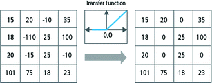
Pictorial representation of ReLU functionality
-
The pooling/subsampling layer reduces the resolution of the features. It makes the features robust against noise and distortion.
-
Fully connected layers are often used as the final layers of a CNN. These layers mathematically sum a weighting of the previous layer of features, indicating the precise mix of “ingredients” to determine a specific target output result. In case of a fully connected layer, all the elements of all the features of the previous layer get used in the calculation of each element of each output feature.

Training is performed using a “labeled” data set of inputs in a wide assortment of representative input patterns that are tagged with their intended output response. Training uses general-purpose methods to iteratively determine the weights for intermediate and final feature neurons. Figure 4 demonstrates the training process at a block level.

Training of neural networks [9]
3 Develop CNN Models for Leaves Recognition
3.1 Extract Leaf Vein Shape
The input data of the model is the image, which normally has three RGB channels. However, in order to reduce the storage capacity, extract vein morphology for network training, we propose to extract vein morphology to the remaining one channel input, which will reduce the number of the weight value (associated with the two remaining channels) that the network must learn.
To perform extract leaf vein shape, the image segmentation process involves converting the image to grayscale, and then using adaptive thresholding techniques to segment the image and extract the vein leaf image.
There are many image processing techniques used to segment the image, many researched extracted vein morphology from images obtained by the camera and using Gabor filters, Colony filters, thresholds, independent component analysis,…
We use adaptive local threshold algorithm that decouples object from background with heterogeneous illumination produces a binary image with adjacent thresholds is the mean (ws) - C, ws is the neighborhood size, C is the constant, in this study we use ws = 10 and C = 0.2, these two results in low noise picture most from images in our experiments. Figure 5, presentation of a result illustrating adaptive local threshold.

Illustrated image with adaptive local threshold to mean (10), C = 0.2
3.2 The CNN Model Classifies Leaves
In the Fig. 6, L1, L2 model, each phase include three transformations. First, the convolution between the input image and n filters (we set n = 100 at L1, n = 250 at L2) is 5 × 5 size. Each filter has a limit size related to a receiving field (5 × 5) in the input image. For each convolution filter generates a feature map. The second transformation is a non-linear function used for all feature maps. We use the ReLU function. Finally, there is a subsampling transformation. In this transformation, each map is divided into a set of non-overlapping 5 × 5 square fields, from each point in that field, which retains only the maximum value (or Max Pool).

CNN model for leaves recognition
The CNN model shown in Fig. 6 have layers that include:
[Conv1 - ReLu - Max pool] → [Conv2 - ReLu - Max pool] → [Conv3 - ReLu] → [Conv4 → FC] → Softmax.
L3, L4 are two convolutional layers to create a fully-enclosed class of filter sizes of 1 × 1 according to Matconvnet’s convention [11]. Finally in the network is a softmax function. It returns the estimated probability of each class, for a particular sample. This layer is fully connected to all the output feature maps of the final convolution layer.
A summary of the network parameters is detailed in Table 1.
The training network updates the network of parameters model. The parameters were optimized using Stochastic gradient descent (SGD) that in contrast performs a parameter update for each training.
4 Experiment and Results
4.1 Experiment Data Sets
In order to test the performance of the vein morphology classification system, we selected three standard sets:
-
Flavia data set [12]: This data set contains 1907 leaf images of 32 different species and 50–77 images per species. Those leaves were sampled on the campus of the Nanjing University and the Sun Yat-Sen arboretum, Nanking, China. Most of them are common plants of the Yangtze Delta, China. The leaf images were acquired by scanners or digital cameras on plain background. The isolated leaf images contain blades only, without petioles.
-
Swedish leaf data set [2]: The Swedish leaf data set has been captured as part of a joined leaf classification project between the Linkoping University and the Swedish Museum of Natural History. The data set contains images of isolated leaf scans on plain background of 15 Swedish tree species, with 75 leaves per species (1125 images in total). This data set is considered very challenging due to its high inter-species similarity.
-
Mekong leaf data set: this data set was collected by us during the study, in the provinces of the Mekong Delta in Vietnam. Images were taken with a leaf camera in the field on a white background with natural light, and include 52 common trees such as fruit trees, wood trees, medicinal plants, ornamental plants… each with 47–110 images, total 3,921 images.
4.2 Augmentation Data
To limit over-model phenomena of the model due to insufficient data. Augmentation data is an effective solution. We increase number of training images by creating three copies of each image after reflection and rotation.
Thus, each original image creates three image augmentation. Data partitioned for experiment is shown in Table 2.
In this study, the input data of model is scanned or taken from leaves of the trees, data is classified into three categories: RGB, graycale and threshold images extract veins morphology, then model the training on these volumes to compare the results. The experimental process is as follows:
-
Data preprocessing: each data set is divided into three categories: RGB, Graycale, Subdivision.
-
Standardized image size: After preprocessing, the image resizes to 160 × 160px to match the input of the network.
-
Image Partition: Each categories is partitioned as shown in Table 2 for experimental purposes.
-
Initialization parameter:
-
Learning rate: set to 0.0001 (greater than fast convergence network but not very good error rate, smaller than slow convergence network).
-
Weight Decay constant (anti-overfitting) = 0.0005;
-
Momentum constant = 0.9.
-
The above constants are chosen based on experimental results for proposed model by trial and error Method. Training time depends on computer resources with GPU or CPU, matlab software and Matconvnet tool.
4.3 Experiment Results
The experiment results are aggregated into each test data set and detail in Tables 3, 4 and 5.
From the experiment results in Tables 3, 4 and 5, we have following comments:
-
The model error rate and test test on RGB data gives better results. However, the storage and training time is longer. On data thresholds that store little data and fast training networks, results equivalent (or less negligible). Augmentation data improves network efficiency, both in terms of model error rate and recognition rate.
-
Random partition of data set as 60% train, 20% val, 20% test of the network give results equivalent compare to 5 fold partition on the Swedish data set. For the Flavia and Mekong data set, 5 fold partition has lower performance network. This happens probably due to data sets have unequal data in each layer.
Comparisons of the results were compiled in [13] with the method of leaves recognition on the Swedish and Flavia data sets in the following Tables 6 and 7. Here, the accuracy is (Number of correct identities/Total leaf of test set) × 100%.
From experiment results with Swedish and Flavia data sets, we can confirm that the CNN-based neural network depth model, which we propose, works very well on classification problem of leaves based on the shape of veins (vein morphology). This result once again confirms the effectiveness and simplicity of the CNN depth geometry model for real-world problems with large data. The recognition process is done by simply building the model and determining the appropriate parameters. The effectiveness of the classification process, recognition is no longer too dependent on finding and identifying image features, a process that takes a lot of time and effort.
5 Conclusion
In this study a novel CNN architecture was proposed for leaf classification task. The model is based on 160 × 160 adaptive threshold images input that obtained from Swedish, Flavia, Mekong leaf dataset. The effect of horizontal reflection and rotation augmentation of data sets is also to further improve the results. The results showed that the proposed architecture for CNN-based leaf classification closely competes with the latest extensive approaches on devising leaf features and classifiers.
In future research, we improve the back propagation algorithm by combining other methods such as genetic algorithms, fuzzy logic, extensive study of network architectures and training algorithms, …
Change the ReLU transfer function with a more flexible function for each class such as ELU (Exponential Linear Unit)… for better training results. The problem of normalizing the size of the subject needs further research to increase its effectiveness on the large and small object images.
References
Oide, M., Ninomiya, S.: Discrimination of soybean leaflet shape by neural networks with image input. Comput. Electorn. Agric. 29(1–2), 59–72 (2000)
Soderkvist, O.J.O.: Computer Vision Classification of Leaves from Swedish Trees. Linkoping University, Linkoping (2001)
Krizhevsky, A., Sutskever, I., Hinton, G.E.: Imagenet classification with depth convolutional neural networks. In: Advances in Neural Information Processing Systems (2012)
Jassmann, T.J., Tashakkori, R., Parry, R.M.: Leaf classification utilizing a convolutional neural network. In: SoutheastCon 2015, pp. 1–3. IEEE (2015)
Wu, Y.-H., Shang, L., Huang, Z.-K., Wang, G., Zhang, X.-P.: Convolutional neural network application on leaf classification. In: Huang, D.-S., Bevilacqua, V., Premaratne, P. (eds.) ICIC 2016. LNCS, vol. 9771, pp. 12–17. Springer, Cham (2016). https://doi.org/10.1007/978-3-319-42291-6_2
He, X., Wang, G., Zhang, X.-P., Shang, L., Huang, Z.-K.: Leaf classification utilizing a convolutional neural network with a structure of single connected layer. In: Huang, D.-S., Jo, K.-H. (eds.) ICIC 2016. LNCS, vol. 9772, pp. 332–340. Springer, Cham (2016). https://doi.org/10.1007/978-3-319-42294-7_29
Sladojevic, S., Arsenovic, M., Anderla, A., Culibrk, D., Stefanovic, D.: Deep neural networks based recognition of plant diseases by leaf image classification. Comput. Intell. Neurosci. 11 (2016)
Artificial Neural Network. Wikipedia. https://en.wikipedia.org/wiki/Artificial_neural_network
Hijazi, S., Kumar, R., Rowen, C.: Using convolutional neural networks for image recognition. IP Group, Cadence (2015). https://ip.cadence.com/uploads/901/cnn_wp-pdf
Vedaldi, A., Lenc, K.: Matconvnet: convolutional neural networks for matlab. In: Proceedings of the 23rd ACM International Conference on Multimedia, pp. 689–692. ACM (2015)
Wu, S.G., Bao, F.S., Xu, E.Y., Wang, Y.X., Chang, Y.F., Xiang, Q.L.: A leaf recognition algorithm for plant classification using probabilistic neural network. In: 2007 IEEE International Symposium on Signal Processing and Information Technology, pp. 11–16. IEEE (2007)
Wäldchen, J., Mäder, P.: Plant species identification using computer vision techniques: a systematic literature review. Arch. Comput. Methods Eng. (2017). https://www.researchgate.net/publication/312147459. ISSN: 1134–3060 (Print) 1886-1784 (Online)
Author information
Authors and Affiliations
Corresponding author
Editor information
Editors and Affiliations
Rights and permissions
Copyright information
© 2018 Springer International Publishing AG, part of Springer Nature
About this paper

Cite this paper
Nguyen Thanh, T.K., Truong, Q.B., Truong, Q.D., Huynh Xuan, H. (2018). Depth Learning with Convolutional Neural Network for Leaves Classifier Based on Shape of Leaf Vein. In: Nguyen, N., Hoang, D., Hong, TP., Pham, H., Trawiński, B. (eds) Intelligent Information and Database Systems. ACIIDS 2018. Lecture Notes in Computer Science(), vol 10751. Springer, Cham. https://doi.org/10.1007/978-3-319-75417-8_53
Download citation
DOI: https://doi.org/10.1007/978-3-319-75417-8_53
Published:
Publisher Name: Springer, Cham
Print ISBN: 978-3-319-75416-1
Online ISBN: 978-3-319-75417-8
eBook Packages: Computer ScienceComputer Science (R0)