
Abstract
Dynamic prediction for pilot situation awareness (SA) is an important issue in aviation safety. This paper presents a dynamic prediction model on the basis of the progressive triggering relationship between low and high-level SA. Six typical cognitive status (“Unnoticed”, “Attention of situation element (SE) but not reaching perception”, “Perception of SE”, “Perception but not matching the best rule”, “Triggering of the best rule” and “Decision making and operation”) were proposed for the description of the cognitive process of SE. Eighteen participants were selected to conduct the flight simulation tasks, and the situation awareness global assessment technique (SAGAT) method was adopted to measure the performance data (including accuracy and response time) at 13 typical time points. Statistical analysis showed that the theoretical value of the proposed SA dynamic prediction model was significantly correlated with accuracy and response time, which validated the model in the flight simulation environment preliminary. The proposed SA dynamic model in flight scenarios can give some references for cockpit’s human-computer interface design and flight tasks optimization assignment.
You have full access to this open access chapter, Download conference paper PDF
Keywords
1 Introduction
Situation awareness (SA) is closely related to aviation safety. The concept of SA firstly appeared in aviation psychology [1]. Since the late 1980s, there has been a growing number of SA-related studies and has drawn considerable attention from academics [2]. After more than 20 years of research and exploration, SA is now one of the most important studies in ergonomics [2,3,4]. SA is not only related to interface design that supports SA, but also to disasters and accidents that lack of SA, especially for dynamic and safety-centric operating environments. The statistical result of aviation accidents revealed that 35.1% non-major accidents and 51.6% major accidents were caused by the failure of pilot’s decision-making, and the main reason for that was the lack of SA or SA error instead of the error in decision-making. SA can be easily lost when the changing situation was not fully understood by flight crew, which may lead to the controlled flight into terrain (CFIT), such as the Air France Flight 447 [2]. In air traffic control tasks, air traffic controllers (ATC) need to keep abreast of the current aircraft dynamics, or else they may have disastrous consequences, and the American Airlines Flight 1493 in 1991 is a typical example [5]. In the field of nuclear power, the maintaining of a good SA is also crucial for operator’s safety operation, especially in emergencies, such as the Three Island Mile accident in 1979 [6].
The concept of SA has been controversial, with more than 30 definitions [7], of which Endsley’s view is more widely accepted. She pointed out that SA includes three levels of perception, comprehension and prediction, namely “perception of environmental components in a large amount of time and space, understanding of its meaning and prediction of the status in the near future” [1]. At present, studies on SA mainly focus on the theoretical models and measurement methods. The construction of the SA theoretical model is one of the current research difficulties [2, 7, 8]. The study of SA mechanism models is an explanation and extension of the definition of SA, which relies significantly on cognitive psychology and gives explanations of the SA formation process in individual brain [2]. The three-level model, perceptual cycle model [9] and theory of activity model [10] are currently recognized as the three main SA mechanism model.
Since the concept of SA emerged, it has also been one of the researchers’ concerns to establish a quantitative computing model for SA [8, 11, 12]. Up to now, researchers have carried out a series of researches on the quantitative calculation model of SA. For example, Wickens et al. established the Attention-Situation Awareness (A-SA) based on the theory of attention distribution to predict performance errors of pilot [11]. Kirlik and Strauss constructed the SA ecological model by assigning ecological validity to the SE (Situation Element) [12]. Entin’s PSM (Performance Sensitivity Model) emphasizes the dynamics of SE and uses sensitive coefficients to reflect the impact of SE on SA [13]. The SA level in the MIDAS (Human Machine Integration Design and Analysis human performance Model) model of Hooey et al. is calculated by the ratio of the actual state SA level to the ideal state SA level. Liu et al. put forward the SA model based on attention resource allocation [15] and ACT-R (Adaptive Control of Thought Rational) cognitive theory, which conducted the prediction of SA level in flight instrument display scenarios [8].
This paper presents a dynamic prediction model that six typical cognitive status (“Unnoticed”, “Attention of SE but not reaching perception”, “Perception of SE”, “Perception but not matching the best rule”, “Triggering of the best rule” and “Decision making and operation”) were used for the description of the cognitive process of SE. A flight simulation experiment was conducted among eighteen participants, and the statistical analysis was used for the validation of SA model. The proposed SA quantification model of individual can be used to assess and improve SA of the current designs, to predict situations where SA losses may occur, and to improve operator performance [11, 16]. In addition, in a typical aviation environment, the individual SA model can be further extended to the assessment of team SA (consisting of flight crews, air traffic controllers, etc.) and system SA (consisting of flight instrumentation, autopilot, etc.) [2].
2 Theoretical Modeling
Assume that there are n SEs (Situation Elements) in the situation at time t, and the operator’s cognitive level to \( SE_{i} \) is \( P_{i} (t) \). \( P_{i} (t) \) stands for operator’s knowledge of \( SE_{i} \) at present and in the future, and a higher \( P_{i} (t) \) indicates a better understanding of the information in the current and future status.
Here SA(t) is the SA level of operator at time t, which is closely related to each relevant \( SEs \). Note that the true value of \( SE_{i} \) at time t is \( O_{i} (t) \), the characterization value in operator’s brain is \( S_{i} (t) \), and then the \( P_{i} (t) \) can be represented by \( S_{i} (t) \), \( O_{i} (t) \) and uncertain errors \( x_{i} (t) \) [14], see Eq. 2.
\( S_{i} (t) \) is related to characterization value \( S_{i} (t - 1) \) and action \( g_{i} (t - 1) \) in previous time, as well as several internal factors \( k_{i} (t) \) (operator’s memory and knowledge) and external factors \( d_{i} (t) \) (physical display characteristics of SE [13]), therefore
Here the external factors \( d_{i} (t) \) work through internal mechanism \( k_{i} (t) \), and thus affect its characterization state [1].
By considering the progressive trigger relationship [1] [8] in cognitive activity, only low-level cognitive activities accumulated to a certain amount can they enter into the next phase of high-level activities, and cause changes in the quality of cognitive level. Therefore, the level of cognition to a certain SE can be regarded as a discrete value changing with the cognitive stages.
As shown in Fig. 1, the cognitive levels were set as follows: (1) Attentional behavior of \( SE_{i} \) did not occur (event \( \overline{ai} \)); (2) Attention behavior occurred but did not reach to perception (event \( ai\overline{bi} \)); (3) Attention occurred and then reach to perception; (4) Pattern matching but failed to trigger the best rule (event \( aibi\overline{ci} \)); (5) The best rule triggered to form an understanding of current state, that is, to reach the corresponding SA2; Or to form an understanding of the future state, that is, to achieve the corresponding SA3 (event \( aibici \)); (6) Decision-making and operation.

Representation of SA level in cognitive process
The cognitive level at time t is determined by the completion state of \( SE_{i} \) in cognitive circuit [14]:
-
(1)
Attention behavior did not occur
There is only a SE may be noticed at time t, and the individual always tends to choose the most valuable one. The higher the value is, the greater the probability is chosen. Note attention behavior of \( SE_{i} \) as event ai, then
$$ p(ai) = f_{i} (t) $$(6)Here \( f_{i} (t) = \hbox{max} (f_{1} (t), \ldots f_{i} (t), \ldots f_{n} (t)) \). If \( SE_{i} \) was unnoticed, then
$$ p(\overline{ai} ) = 1 - f_{i} (\text{t}) $$(7)There is an updating characteristics in working memory, although theoretically the characterization value of \( SE_{i} \) in operator’s brain should be maintained in time \( t - \tau \). So,
$$ S_{i} ({\text{t}}) = S_{i} ({\text{t}} - \tau ) \times {\text{e}}^{{ - k_{1} \tau }} $$(8)where \( k_{1} \) reflects the speed of information updating in working memory of individual. The following \( k_{1} = 0 \) indicates that the \( SE_{i} \) at time \( t - 1 \) was fully remembered by individual; \( \tau \) reflects the forgotten time of \( SE_{i} \), and the unit time was set as 1 below. It can be seen from Fig. 2 that the \( SE_{i} \) has been characterized in a total of 10 cognitive circuits. Since no attention occurs, the cognitive status is not updated at this time, and the memory at time \( t - 1 \) continues to be maintained. The cognitive status value on each line is as follows:
$$ road_{j} S_{i} (t) = road_{j} S_{i} (t - 1) \times e^{{ - k_{1} }} $$(9)Fig. 2. 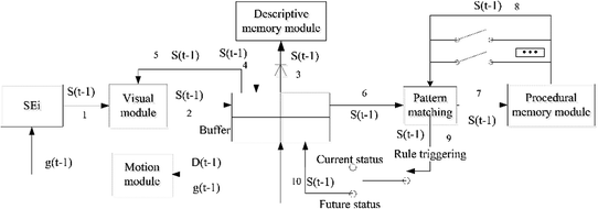
Description of SA cognitive process
At this time, the cognitive level of \( SE_{i} \) exists in the following two situations: (1) When \( \frac{{O_{i} (\text{t}) - S_{i} (\text{t})}}{{O_{i} (\text{t}) + \varsigma_{min} }} = \frac{{O_{i} (\text{t}) - e^{{ - k_{1} }} S_{i} (\text{t}{ - }1)}}{{O_{i} (\text{t}) + \varsigma_{min} }} \le \Delta \), the difference between \( S_{i} (\text{t}) \) in brain at time \( t - 1 \) and \( O_{i} (\text{t}) \) at time t is considered to be within an acceptable error range \( \Delta \). So the cognitive level is \( P_{i} (t) = \sum\limits_{j = 1}^{10} {road_{j} \frac{1}{10} \times \frac{{S_{i} (t)}}{{O_{i} (t)}}} = \frac{{S_{i} (t - 1) \times e^{{ - k_{1} }} }}{{O_{i} (t)}} \). (2) When \( \frac{{O_{i} (\text{t}) - S_{i} (\text{t})}}{{O_{i} (\text{t}) + \varsigma_{{_{min} }} }} = \frac{{O_{i} (\text{t}) - e^{{ - k_{1} }} S_{i} (\text{t} - 1)}}{{O_{i} (\text{t}) + \varsigma_{min} }} > \Delta \), then the difference between \( S_{i} (\text{t}) \) in brain at time \( t - 1 \) and \( O_{i} (\text{t}) \) at time t is considered to be beyond an acceptable error range \( \Delta \).
-
(2)
Attention but not reach perception
Selective attention occurs at time t, and the visual module obtains the new \( S_{i} (t) \) of \( SE_{i} \) with probability of \( f_{i} (t) \) and passes it to the buffer module. The buffer module accesses the descriptive module to extract the corresponding descriptive knowledge. However, the amount of activation \( AC_{i} \) does not reach the threshold and cannot form a perception, the probability is:
$$ p(ai\overline{bi} ) = p(ai) \times p(\overline{bi} /ai) = f_{i} (t) \times p(\overline{bi} /ai) = f_{i} (t)(1 - p(bi/ai)) $$(10)Then probability that selectively attention of \( SE_{i} \) may be occurred at time t is:
$$ f_{i} (t) = {{A_{i} (t)} \mathord{\left/ {\vphantom {{A_{i} (t)} {\sum\limits_{i = 1}^{n} {A_{i} (t)} }}} \right. \kern-0pt} {\sum\limits_{i = 1}^{n} {A_{i} (t)} }} $$(11)where \( A_{i} (t) \) is calculated on the basis of multiple-resource theory [17]. In this case, the cognitive status of line 1–2 is \( S_{i} (t) = O_{i} (t) \), and the value of line 3–10 is not updated, and the memory of the previous time is maintained. At this time, the cognitive status is \( S_{i} (t) = S_{i} (t - 1) \times e^{{ - k_{1} }} \). Similarly, two cognitive level of \( SE_{i} \) were existed: \( P_{i} (t) = 0.2 + \sum\limits_{j = 3}^{10} {\frac{1}{10} \times \frac{{S_{i} (t - 1) \times e^{{ - k_{1} }} }}{{O_{i} (t)}}} \) or \( P_{i} (t) = 0.2 \).
-
(3)
Attention and reach to perception
If \( AC_{i} > Lim \), then the perception of \( S_{i} (t) \) is formed, that is, to reach the SA1. The probability is
$$ p(aibi) = p(ai)p(bi/ai) = \frac{{f_{i} }}{{1 + e^{{ - (AC_{i} ({\text{t}}) - \tau )/s}} }} $$(12)In this case, the cognitive status of line 1–5 is updated and read a new value, 6–10 remained the same as time \( t - 1 \). The cognitive level of \( SE_{i} \) is \( P_{i} (t) = 0.5 + \sum\limits_{j = 6}^{10} {\frac{1}{10} \times \frac{{S_{i} (t - 1) \times e^{{ - k_{1} }} }}{{O_{i} (t)}}} \) or \( P_{i} (t) = 0.5 \).
-
(4)
Pattern matching
The buffer passes the value of new status to the procedural memory module, and to match the corresponding procedural knowledge with varieties of rules: \( U_{1} = P_{1} G - C_{1} \); \( U_{2} = P_{2} G - C_{2} \). However, the best rules have not yet selected and triggered at this point, then the probability of occurrence to this situation is:
$$ p(aibi\overline{ci} ) = p(aibi)p(\overline{ci} /aibi) = p(aibi)(1 - p(ci/aibi)) $$(13)In this case, line 1–5 is updated, line 6–10 is maintained. Then \( P_{i} (t) = 0.8 + \sum\limits_{j = 9}^{10} {\frac{1}{10} \times \frac{{S_{i} (t - 1) \times e^{{ - k_{1} }} }}{{O_{i} (t)}}} \) or \( P_{i} (t) = 0.8 \).
-
(5)
Triggering of the best rule
When the pattern matches the best rule at this time and is triggered by the rule to form an understanding of \( S_{i} (t) \) at present, SA2 or SA3 is considered to be reached; then
$$ p(aibici) = p(aibi)p(ci/aibi) = \frac{{f_{i} }}{{1 + e^{{ - (AC_{i} ({\text{t}}) - \tau )/s}} }}\frac{{e^{{U_{i} /\theta }} }}{{\sum\limits_{l}^{m} {e^{{U_{l} /\theta }} } }} $$(14)Now line 1–10 is updated, \( P_{i} (t) = \sum\limits_{j = 1}^{10} {road_{j} \frac{1}{10} \times \frac{{S_{i} (t)}}{{O_{i} (t)}}} = 1 \).
-
(6)
Decision making and operation
According to the formed SA, instructions \( D_{i} (t) \) related to current situation was transmitted to motion module by pilot, then:
$$ D_{i} (t) = f(D_{i} (t - 1),S_{i} (t),k_{i} (t)) $$(15)Now line 1–10 is updated, \( P_{i} (t) = 1 \). According to the decision signals, the motion module makes a certain action to \( g_{i} (t) \), and the action feeds back to the buffer module.
$$ g_{i} (t) = f(g_{i} (t - 1),D(t),S_{i} (t),k_{i} (t)) $$(16)Suppose there are n SEs, where \( e_{i} \) represents the influence coefficient of each SE’s cognitive level to current SA, and its value is related to multiple factors. Research indicated that the sensitivity coefficient is related to the average task load \( \overline{mw}_{k} \), the presentation interval time of information \( \Delta T_{it} \), processing time of information \( \Delta T_{pt} \) [17].
$$ e_{i} = f(\overline{mw}_{i} ,T_{i} ) = \overline{mw}_{i} *\Delta T_{it} *\Delta T_{pt} $$(17)Then the final expression of SA is
$$ SA(t) = \sum\limits_{i = 1}^{n} {e_{i} P_{i} (t)} = e_{1} P_{1} (t) + e_{2} P_{2} (t) \ldots e_{i} P_{i} (t) + e_{n} P_{n} (t) $$(18)

3 Experimental Validation of SA Model
Two parts were mainly included in the experimental verification of SA model: design of typical situation and achievement of performance measurement. Interface simulation models and design of experimental scheme under simulated flight conditions were included in typical situation. The experimental data were collected by the Situation Awareness Global Assessment Technique (SAGAT) [1].
3.1 Design of Typical Situation
A high-fidelity simulation flight platform was built based on Flight Gear 3.4.0 software in laboratory environment, which includes the Primary Flight Display (PFD), the Navigation Display (ND) panel, and the Engine Indication and Crew Alerting System (EICAS)), shown as Fig. 3(a)–(c). The flight information display interface was presented in three 17-in. LCD screen (see Fig. 3(d)), with the average screen brightness of 120 cd/m2, the resolution of 1280 × 1024, the ambient light of 600 lx. The Saitek Yoke civil aviation flight joystick system was used to complete the flight operations.

Experiment scenario and interface design
3.2 Participants
Eighteen participants (average was 22.6 years) were selected to carry out flight simulation tasks, all of whom were simulated pilot who had a good aviation background from Beihang university. They were both in good health, right handed, and with a normal vision or corrected vision.
3.3 Experimental Design
The flight situation which composed of flight mission and interface display factors was mainly investigated in this experiment. The display area was divided into 3 AOIs, namely, PFD (AOI 1), ND (AOI 2) and EICAS (AOI 3). Each participant needs to complete a traffic-pattern flight, in which the “three-four turning and auto-alignment” phase was chosen to validate the model.
All participants were required to have adequate simulated flight training and the formal testing was commenced after the flight operations and experimental procedures had been fully mastered. The corresponding scores for flight task operations and average task in multiple-resource load [18] were shown in Table 1.
A single-factor within-subject design was used in the validation, and the dynamic changes of SA level in different freezing time points which consisting of task operations and instrument displays in the flight scenarios was the independent variable. During the experiment, the experimental interface froze at different experimental time points and the corresponding freezing questions occurred. The participant needs to make response with the mouse within a given time. The corresponding freezing problems are shown in Table 2. The instrumental importance of each AOI was set according to the flight situation [17], and the information expectation was given in the start of the experiment, showed in Table 2.
4 Experimental Results and Analysis
4.1 Theoretical Value of Dynamic SA Model and the Experiment Value
The interface design, attention mobility, information expectation and information value in the three monitored AOIs by experimental interface model were calculated, showed in Table 3 [8].
\( P(bi/ai) \), \( P(ci/bi) \), \( P(aibi) \), \( P(aibici) \) were calculated by Eqs. 12 and 14 respectively, and combined with the Eq. 17 to obtain the SA level at each time point, the results were shown in Table 4.
4.2 Correlation Analysis
Based on the validation method of SA model used by Wickens et al. [11], a Pearson correlation analysis was performed between predictive value of SA model and experimental measurement results. The variation of SA predictive value, response time and accuracy in different time points were shown in Figs. 4, 5 and 6.

Variation of SA predictive value in different time points

Variation of response time in different time points

Variation of accuracy in different time points
The statistical results showed that there was a significant moderate correlation between SA predictive value and accuracy in performance measurement (r = 0.642, P = 0.018) and a significant moderate correlation with SAGAT response (r = −0.554, p = 0.049), which has verified the validity of the model to a certain extent.
5 Conclusion
In conclusion, a new quantitative generation model of SA was proposed in this study. By considering the progressive trigger relationship between low and high-level SA, six discrete values was divided to the cognitive level of a certain information component; the sensitivity coefficient was calculated on multiple-resource theory, and the SA level was then calculated on the basis of conditional probability theory. The verification of SA model is completed on the built simulation platform. Based on the different display instrument, the “three-four turning and auto-alignment” is selected for situation to be analyzed. The verification results showed that the proposed SA model has a certain validity.
References
Endsley, M.R.: Toward a theory of situation awareness in dynamic systems. Hum. Fact.: J. Hum. Fact. Ergon. Soc. 37(1), 32–64 (1995)
Stanton, N.A., Salmon, P.M., Walker, G.H., Salas, E., Hancock, P.A.: State-of-science: situation awareness in individuals, teams and systems. Ergonomics 60(4), 449–466 (2017)
Wickens, C.D.: Situation awareness: review of Mica Endsley’s 1995 articles on situation awareness theory and measurement. Hum. Fact. 50(3), 397–403 (2008)
Salmon, P.M., Stanton, N.A.: Situation awareness and safety: contribution or confusion? Situation awareness and safety editorial. Saf. Sci. 56(7), 1–5 (2013)
Wickens, C.D., Gutzwiller, R.S., Santamaria, A.: Discrete task switching in overload: a meta-analyses and a model. Int. J. Hum.-Comput. Stud. 79(C), 79–84 (2015)
She, M.R., Li, Z.Z.: Design and evaluation of a team mutual awareness toolkit for digital interfaces of nuclear power plant context. Int. J. Hum.-Comput. Interact. 33(9), 1–12 (2017)
Salmon, P.M.: Distributed situation awareness: advances in theory, measurement and application to team work. Dissertation, Brunel University, London (2008)
Liu, S., Wanyan, X.R., Zhuang, D.M.: Modeling the situation awareness by the analysis of cognitive process. Bio-Med. Mater. Eng. 24(6), 2311–2318 (2014)
Smith, K., Hancock, P.A.: Situation awareness is adaptive, externally directed consciousness. Hum. Fact.: J. Hum. Fact. Ergon. Soc. 37(1), 137–148 (1995)
Bedny, G., Meister, D.: Theory of activity and situation awareness. Int. J. Cogn. Ergon. 3(1), 63–72 (1999)
Wickens, C.D., Mccarley, J.S., Alexander, A.L., Thomas, L.C., Ambinder, M., Zheng, S.: Attention-situation awareness (A-SA) model of pilot error. In: Foyle, D.C., Hooey, B.L. (eds.) Hum Performance Modeling in Aviation, pp. 213–242. Lawrence Erlbaum, Mahwah (2008)
Kirlik, A., Strauss, R.: Situation awareness as judgment I: statistical modeling and quantitative measurement. Int. J. Ind. Ergon. 36(5), 463–474 (2006)
Entin, E.B., Serfaty, D., Entin, E.E.: Modeling and measuring situation awareness for target-identification performance. In: Garland, D.J., Endsley, M.R. (eds.) Experimental Analysis and Measurement of Situation Awareness, pp. 233–242. Embry-Riddle Aeronautical University Press, Daytona Beach (1995)
Hooey, B.L., Gore, B.F., Wickens, C.D., Scott-Nash, S., Salud, E., Foyle, D.C.: Modeling pilot situation awareness. In: Cacciabue, P.C., Hjälmdahl, M., Luedtke, A., Riccioli, C. (eds.) Human Modeling in Assisted Transportation, pp. 207–214. Springer, Heidelberg (2010). https://doi.org/10.1007/978-88-470-1821-1_22
Liu, S., Wanyan, X.R., Zhuang, D.M., Lu, S.C.: Situational awareness model based on attention allocation. J Beijing Univ. Aeronaut. Astronaut. 40(08), 1066–1072 (2014). (in Chinese)
Stanton, N.A., Chambers, P.R.G., Piggott, J.: Situational awareness and safety. Saf. Sci. 39(3), 189–204 (2001)
Feng, C.Y., Wanyan, X.R., Chen, H., Zhuang, D.M.: Research on situation awareness model and its application based on multiple-resource load theory. J. Beijing Univ. Aeronaut. Astronaut. (2018). (in Chinese). https://doi.org/10.13700/j.bh.1001-5965.2017.0532
Liang, S.F.M., Rau, C.L., Tsai, P.F., Chen, W.S.: Validation of a task demand measure for predicting mental workloads of physical therapists. Int. J. Ind. Ergon. 44(5), 747–752 (2014). https://doi.org/10.1016/j.ergon.2014.08.002
Acknowledgement
This study was financially co-supported by the jointly program of National Natural Science Foundation of China and Civil Aviation Administration of China (No. U1733118), as well as the National Natural Science Foundation of China (No. 71301005).
Author information
Authors and Affiliations
Corresponding author
Editor information
Editors and Affiliations
Rights and permissions
Copyright information
© 2018 Springer International Publishing AG, part of Springer Nature
About this paper

Cite this paper
Feng, C., Wanyan, X., Liu, S., Zhuang, D., Wu, X. (2018). Dynamic Prediction Model of Situation Awareness in Flight Simulation. In: Harris, D. (eds) Engineering Psychology and Cognitive Ergonomics. EPCE 2018. Lecture Notes in Computer Science(), vol 10906. Springer, Cham. https://doi.org/10.1007/978-3-319-91122-9_10
Download citation
DOI: https://doi.org/10.1007/978-3-319-91122-9_10
Published:
Publisher Name: Springer, Cham
Print ISBN: 978-3-319-91121-2
Online ISBN: 978-3-319-91122-9
eBook Packages: Computer ScienceComputer Science (R0)