The Algebraic Group Model and its Applications

Abstract

One of the most important and successful tools for assessing hardness assumptions in cryptography is the Generic Group Model (GGM). Over the past two decades, numerous assumptions and protocols have been analyzed within this model. While a proof in the GGM can certainly provide some measure of confidence in an assumption, its scope is rather limited since it does not capture group-specific algorithms that make use of the representation of the group.

To overcome this limitation, we propose the Algebraic Group Model (AGM), a model that lies in between the Standard Model and the GGM. It is the first restricted model of computation covering group-specific algorithms yet allowing to derive simple and meaningful security statements. To prove its usefulness, we show that several important assumptions, among them the Computational Diffie-Hellman, the Strong Diffie-Hellman, and the interactive LRSW assumptions, are equivalent to the Discrete Logarithm (DLog) assumption in the AGM. On the more practical side, we prove tight security reductions for two important schemes in the AGM to DLog or a variant thereof: the BLS signature scheme and Groth’s zero-knowledge SNARK (EUROCRYPT 2016), which is the most efficient SNARK for which only a proof in the GGM was known. Our proofs are quite simple and therefore less prone to subtle errors than those in the GGM.

Moreover, in combination with known lower bounds on the Discrete Logarithm assumption in the GGM, our results can be used to derive lower bounds for all the above-mentioned results in the GGM.

1 Introduction

Starting with Nechaev [Nec94] and Shoup [Sho97], much work has been devoted to studying the computational complexity of problems with respect to generic group algorithms over cyclic groups [BL96, MW98, Mau05]. At the highest level, generic group algorithms are algorithms that do not exploit any special structure of the representation of the group elements and can thus be applied in any cyclic group. More concretely, a generic algorithm may use only the abstract group operation and test whether two group elements are equal. This property makes it possible to prove information-theoretic lower bounds on the running time for generic algorithms. Such lower bounds are of great interest since for many important groups, in particular for elliptic curves, no helpful exploitation of the representation is currently known.

The class of generic algorithms encompasses many important algorithms such as the baby-step giant-step algorithm and its generalization for composite-order groups (also known as Pohlig-Hellman algorithm [HP78]) as well as Pollard’s rho algorithm [Pol78]. However, part of the common criticism against the generic group model is that many algorithms of practical interest are in fact not generic. Perhaps most notably, index-calculus and some factoring attacks fall outside the family of generic algorithms, as they are applicable only over groups in which the elements are represented as integers.

Another example is the “trivial” discrete logarithm algorithm over the additive group , which is the identity function.

With this motivation in mind, a number of previous works considered extensions of the generic group model [Riv04, LR06, AM09, JR10]. Jager and Rupp [JR10] considered assumptions over groups equipped with a bilinear map $e:\mathbb {G}_1\times \mathbb {G}_2\longrightarrow \mathbb {G}_3$, where $\mathbb {G}_1$ and $\mathbb {G}_2$ are modeled as generic groups, and $\mathbb {G}_3$ is modeled in the Standard Model. (This is motivated by the fact that in all practical bilinear groups, $\mathbb {G}_1$ and $\mathbb {G}_2$ are elliptic curves whereas $\mathbb {G}_3$ is a sub-group of a finite field). However, none of these models so far capture algorithms that can freely exploit the representation of the group. In this work, we propose a restricted model of computation which does exactly this.

1.1 Algebraic Algorithms

Let $\mathbb {G}$ be a cyclic group of prime order p. Informally, we call an algorithm $\mathsf {A}_\mathsf {alg}$ algebraic if it fulfills the following requirement: whenever $\mathsf {A}_\mathsf {alg}$ outputs a group element $\mathbf {Z}\in \mathbb {G}$, it also outputs a “representation” such that $\mathbf {Z}=\prod _i\mathbf {L}_i^{z_i}$, where is the list of all group elements that were given to $\mathsf {A}_\mathsf {alg}$ during its execution so far.

Such algebraic algorithms were first considered by Boneh and Venkatesan [BV98] in the context of straight-line programs computing polynomials over the ring of integers $\mathbb {Z}_n,$ where $n=pq$. Later, Paillier and Vergnaud [PV05] gave a more formal and general definition of algebraic algorithms using the notion of an extractor algorithm which efficiently computes the representation $\vec z$.

In our formalization of algebraic algorithms, we distinguish group elements from all other parameters at a syntactical level, that is, other parameters must not depend on any group elements. This is to rule out pathological exploits of the model, see below.

While this class of algebraic algorithms certainly captures a much broader class of algorithms than the class of generic algorithms (e.g., index-calculus algorithms), it was first noted in [PV05] that the class of algebraic algorithms actually includes the class of generic algorithms.

Algebraic algorithms have mostly been studied so far in the context of proving impossibility results [BV98, Cor02, PV05, BMV08, GBL08, AGO11, KMP16], i.e., to disprove the existence of an algebraic security reduction between two cryptographic primitives (with certain good parameters). Only quite recently, a small number of works have considered the idea of proving statements with respect to algebraic adversaries [ABM15, BFW16].

1.2 Algebraic Group Model

We propose the algebraic group model (AGM) — a computational model in which all adversaries are modeled as algebraic. In contrast to the GGM, the AGM does not allow for proving information-theoretic lower bounds on the complexity of an algebraic adversary. Similar to the Standard Model, in the AGM one proves security implications via reductions. Specifically, $H \Rightarrow _{\mathsf {alg}} G$ for two primitives H and G means that every algebraic adversary $\mathsf {A}_\mathsf {alg}$ against G can be transformed into an algebraic adversary $\mathsf {B}_\mathsf {alg}$ against H with (polynomially) related running times and success probabilities. It follows that if H is secure against algebraic adversaries, so is G. While algebraic adversaries have been considered before (see above), to the best of our knowledge, our work is the first to provide a clean and formal framework for security proofs with respect to algebraic adversaries. We elaborate further on our model below.

Concrete Security Implications in the AGM. Indeed, one can exploit the algebraic nature of an adversary in the AGM to obtain stronger security implications than in the Standard Model. The first trivial observation is that the classical knowledge of exponent assumption¹ [Dam92] holds by definition in the AGM.

We are able to show that several important computational assumptions are in fact equivalent to the Discrete Logarithm assumption over prime-order groups in the AGM, including the following:

• Diffie-Hellman assumption [DH76]

• (Interactive) strong Diffie-Hellman assumption [ABR01]

• (Interactive) LRSW assumption [LRSW99, CL04].

The significance of the Strong Diffie-Hellman Assumption comes from its equivalence to the IND-CCA security of Hashed ElGamal encryption (also known as Diffie-Hellman Integrated Encryption Standard) in the random oracle model [ABR01]. The LSRW assumption (named its authors [LRSW99]) is of importance since it is equivalent to the (UF-CMA) security of Camenisch-Lysyanskaya (CL) signatures [CL04]. CL signatures are a central building block for anonymous credentials [CL04, BCL04, BCS05], group signatures [CL04, ACHdM05], e-cash [CHL05], unclonable functions [CHK+06], batch verification [CHP07], and RFID encryption [ACdM05]. Via our results, the security of all these schemes is implied by the discrete logarithm assumption in the AGM.

Our result can be interpreted as follows. Every algorithm attacking one of the above-mentioned problems and schemes must solve the standard discrete logarithm problem directly, unless the algorithm relies on inherently non-algebraic operations. In particular, powerful techniques such as the index-calculus algorithms do not help in solving these problems any better then they do for solving the discrete logarithm problem directly.

Moreover, we show the tight equivalence of the security of the following schemes to the underlying hardness assumptions in the AGM:

• IND-CCA1 (aka lunchtime) security of the standard ElGamal Encryption to a parametrized variant of Decisional Diffie-Hellman assumption where in addition to $g^x,g^y$ the adversary receives $g^{x^2},\ldots ,g^{x^q}$, where q is the maximal number of decryption queries.

• The UF-CMA security of the BLS signature scheme [BLS04] to the discrete logarithm problem in the random oracle model. Previous reductions non-tightly reduced from the CDH problem, with a tightness loss linear in the number of signing queries. This loss is known to be inherent [Cor02, KK12], even in the random oracle model.

• The security of the so far most efficient zero-knowledge SNARK scheme by Groth [Gro16] to a parametrized variant of the discrete logarithm problem, where in addition to $g^x$ the adversary receives $g^{x^2},\ldots ,g^{x^{2n-1}}$, where n is the degree of the quadratic arithmetic programs. The only previous proof of the security of this scheme is in the generic group model.

Relation to the Generic Group Model. The AGM is stronger (in the sense that it puts more restrictions on the attackers) than the Standard Model, but weaker than the GGMl. In spite of this, all of our reductions are purely generic algorithms. As mentioned above, any generic algorithm can be modeled within the AGM. In particular, combining arbitrary generic operations with algebraic ones will yield an algebraic algorithm. This suggests the following idea. Let H and G be two computational problems and let $\mathsf {A}_\mathsf {alg}$ be an algebraic algorithm that solves problem G. If we can convert $\mathsf {A}_\mathsf {alg}$ by means of a generic reduction algorithm $\mathsf {R}_\mathsf {gen}$ into an algorithm $\mathsf {B}_\mathsf {alg}$ for problem H, then clearly, $\mathsf {B}_\mathsf {alg}$ is also an algebraic algorithm. However, we obtain an even stronger statement for free: Namely, if $\mathsf {A}_\mathsf {gen}$ is a generic algorithm solving G, then $\mathsf {B}_\mathsf {gen}$ is a generic algorithm solving H. This means that results in the AGM directly carry over to the GGM.

For this reason, we believe that our model offers an alternative, perhaps simpler method of proving the hardness of computational problems within the GGM. This applies in particular to interactive assumptions, which can be rather difficult to analyze in the GGM. For example, we prove that the discrete logarithm assumption implies the LRSW assumption in the AGM. As the discrete logarithm assumption holds in the GGM, we instantly obtain that the LRSW assumption holds in the GGM. The first (rigorous) proof of the LRSW assumption within the GGM was presented in the work of [BFF+14] (the original work [LRSW99] provided only a proof sketch), but was derived from a more general theorem and proven using an automated proof verification tool. We hope that our proof can offer some additional insight over the proof of [BFF+14]. Another example is our tight equivalence of the IND-CCA1 security of ElGamal and our parametrized variant of the Decisional Diffie-Hellman (DDH) assumption in the algebraic group model. Together with the known generic $\sqrt{p/q}$ attack on ElGamal [BG04] for certain primes p (see also [Che06]), our result proves the tight generic bound $\tilde{\varTheta }(\sqrt{p/q})$ on the complexity of breaking IND-CCA1 security of ElGamal in the GGM.

We also remark that proofs in the AGM have an inherently different interpretation than proofs in the GGM. To analyze the hardness of an assumption in the GGM, one must explicitly augment the model by any functionality that is offered by the structure of the group. As a simple example, let us consider a group $\mathbb {G}$ which is equipped with a symmetric bilinear map $e:\mathbb {G}\times \mathbb {G}\longrightarrow \mathbb {G}_T$. The bilinear map can be modeled in the GGM via an oracle. However, it is not clear whether e can be used to gather even further information about the elements of $\mathbb {G}$. Though it is widely believed that this is not the case, a proof in the GGM provides no answer to this question, because the GGM itself is based on the conjecture that e does not offer any functionality beyond a bilinear map. In contrast, the AGM captures any such exploit without the need of having to model it explicitly and considers the relation between two problems instead of their individual hardness. This means that if one can reduce H to G in the AGM and H is conjectured to remain hard with respect to algebraic algorithms, even when given e, then also G remains hard. No similar statement can be inferred in the GGM. Thus, the AGM allows for a more fine grained assessment of the hardness of computational problems than the GGM.

The gap between the two models becomes even more apparent if one considers structural properties of $\mathbb {G}$ which cannot be meaningfully modeled as an oracle in the GGM. As an example, consider the Jacobi symbol, which was shown to be generically hard to compute in [JS09]. Indeed, it was left as an open problem in [AM09] to re-examine the equivalence of factoring and breaking the RSA assumption if an additional oracle for the Jacobi symbol were given. Though their results are stated in the generic ring model rather than the GGM, it seems they are similarly confronted with the issue of explicitly modeling such an oracle.

Limitations of the AGM. As already noted, one of the main benefits of our model over the GGM is the ability to reason about algorithms that arbitrarily exploit the structure of the group. So which algorithms are not covered in this manner? Obviously, outputting an obliviously sampled group element (with unknown representation) is forbidden. This coincides with the GGM of Maurer [Mau05] and which also excludes the possibility of obliviously sampling a random group element. For this reason, our model is strictly weaker than the one from [Mau05] in the sense that any security reduction derived in Maurer’s GGM also holds in the AGM. In contrast, the GGM defined by Shoup [Sho97] does allow for such a sampling process. Similar to Maurer’s GGM, we can allow obliviously sampling a random group element $\mathbf {X}$ through an additional oracle $\mathsf {O}_{}()$ that can be called during the execution of $\mathsf {A}_\mathsf {alg}$. By definition, the outputs of $\mathsf {O}_{}()$ are added to the list . We have thus argued that both versions of the GGM (i.e., the ones by Maurer and Shoup) are strictly stronger than the AGM. Also note that simulating $\mathsf {O}_{}()$ to $\mathsf {A}_\mathsf {alg}$ as part of a reduction is straight-forward and always possible; the reduction simply samples r and returns $g^r$ to the adversary. As the reduction knows r, adding $\mathsf {O}_{}()$ to an experiment does not change it and is completely without loss of generality. From a practical point of view, it seems that generating and outputting a random group element without knowing a representation is generally not of much help. We therefore believe that the AGM captures most algorithms of practical interest.

1.3 Related Work and Open Questions

We have already mentioned the semi generic group model (SGGM) [JR10] as related work, but we discuss here some key differences of their model to ours in more detail. First, the SGGM is a very restrictive model in the sense that the class of problems it captures is limited. The main theorem of [JR10] (Theorem 3) holds only for pairing-based computational problems in which the output consists of a single element in either one of the base groups. In contrast, the AGM does not require a pairing group setting and thus applies to a much broader class of computational problems. Second, by extending the AGM to pairing groups, we are able to model all three groups as algebraic and reason again about a broader class of problems, in which the output can also consist of elements in the target group. To extend the AGM to the pairing setting, we allow the algebraic adversary to compute any element in the target group by applying the pairing to elements in the respective base groups.

Dent [Den02] shows that the generic group model as proposed Shoup [Sho97] inherits the known weaknesses in the random oracle model [CGH98]. Thus, there exist schemes which can be proven secure in Shoup’s GGM, but are pathologically insecure when viewed in the standard model. An interesting open question is whether the AGM bears similar weaknesses. A promising line of research related to this question has recently been initiated by Bitansky et al. [BCPR16]. Namely, they show that indistinguishability obfuscation (iO) implies the existence of non-extractable one-way functions. If these non-extractable one-way functions were furthermore algebraic (such as the knowledge of exponent assumption [Dam92]), then this would invalidate the AGM (under the assumption that iO exists).

Another promising direction for future research is to prove further reductions between common computational assumptions in the AGM. In particular, it would be interesting to classify different such assumptions within the AGM, for example along the lines of work [SS01, Kil01, Boy08, JR15, CM14, MRV16, GG17].

We leave it as an open problem to come up with a meaningful formalization of the AGM for decisional assumptions. At a technical level, the main difficulty in this task arises from the fact that an algorithm, i.e., distinguisher, in a decisional problem is asked to output a bit rather than a group element. Therefore, such an algorithm is trivially considered algebraic in our framework. It would therefore be interesting to develop a model which captures the algebraic properties of such algorithms in more detail.

A further potential for follow-up work would be to investigate whether it is possible to automate proofs in the AGM. Indeed, for the case of the GGM this has been considered in [BFF+14, ABS16] and it would be interesting to see if similar automated tools can be derived for the AGM.

Finally, we remark that all of our results require prime-order groups and do not yet extend to the setting of pairing groups. When generalizing our results to composite-order groups, we expect to encounter the following technical difficulty: Given, e.g., an equation of the form $ax\equiv _n b$, where n is composite, there might be (exponentially) many solutions for the unknown x in case $\mathsf {gcd}(a,n) > 1$. This interferes with the proof strategies presented in this work and requires a more involved analysis. In fact, proving a reduction from the discrete logarithm problem to the CDH problem in the AGM for group orders containing multiple prime factors (e.g., $n=p^2$) is excluded by [MW98]. Hardness bounds in the GGM for composite-order groups have been considered in [Sho97, MW98, Mau05]. Generalizing the GGM to pairing groups has been the subject, e.g., of the works of [Boy08, KSW08, RLB+08]. Extending the AGM to either one of these regimes is an interesting line of research for future work.

2 Algebraic Algorithms

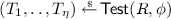
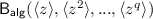
Algorithms. We denote by the uniform sampling of the variable s from the (finite) set S. All our algorithms are probabilistic (unless stated otherwise) and written in uppercase letters $\mathsf {A},\mathsf {B}$. To indicate that algorithm $\mathsf {A}$ runs on some inputs $(x_1,\ldots ,x_n)$ and returns y, we write . If $\mathsf {A}$ has access to an algorithm $\mathsf {B}$ (via oracle access) during its execution, we write .

Security games. We use a variant of (code-based) security games [BR04, Sho04]. In game $\mathbf {G}_{par}$ (defined relative to a set of parameters $par$), an adversary $\mathsf {A}$ interacts with a challenger that answers oracle queries issued by $\mathsf {A}$. It has a main procedure and (possibly zero) oracle procedures which describe how oracle queries are answered. We denote the output of a game $\mathbf {G}_{par}$ between a challenger and an adversary $\mathsf {A}$ via $\mathbf {G}_{par}^{\mathsf {A}}.$ $\mathsf {A}$ is said to win if $\mathbf {G}_{par}^{\mathsf {A}}=1.$ We define the advantage of $\mathsf {A}$ in $\mathbf {G}_{par}$ as $\mathbf {Adv}^{\mathbf {G}}_{par,\mathsf {A}}:=\Pr \big [\mathbf {G}_{par}^{\mathsf {A}}=1\big ]$ and the running time of $\mathbf {G}_{par}^{\mathsf {A}}$ as .

Security Reductions. Let $\mathbf {G},\mathbf {H}$ be security games. We write if there exists an algorithm $\mathsf {R}$ (called $(\varDelta _{\varepsilon },\varDelta _t)$-reduction) such that for all algorithms $\mathsf {A}$, algorithm $\mathsf {B}$ defined as $\mathsf {B}:=\mathsf {R}^{\mathsf {A}}$ satisfies

2.1 Algebraic Security Games and Algorithms

We consider algebraic security games $\mathbf {G}_{\mathcal {G}}^{}$ for which we set $par$ to a fixed group description $\mathcal {G}=(\mathbb {G},g,p)$, where $\mathbb {G}$ is a cyclic group of prime order p generated by g. In algebraic security games, we syntactically distinguish between elements of group $\mathbb {G}$ (written in bold, uppercase letters, e.g., $\mathbf {A}$) and all other elements, which must not depend on any group elements. As an example of an algebraic security game, consider the Computational Diffie-Hellman game $\mathbf {cdh}_{\mathcal {G}}^{\mathsf {A}}$, depicted in Fig. 1 (left).

Fig. 1.

Left: Algebraic game $\mathbf {cdh}^{}{}$ relative to group description $\mathcal {G}=(\mathbb {G}, g,p)$ and adversary $\mathsf {A}$. All group elements are written in bold, uppercase letters. Right: Algebraic game $\mathbf {cdh}^{}{}$ relative to group description $\mathcal {G}=(\mathbb {G}, g,p)$ and algebraic adversary $\mathsf {A}_\mathsf {alg}$. The algebraic adversary $\mathsf {A}_\mathsf {alg}$ additionally returns a representation $\vec z=(a,b,c)$ of $\mathbf {Z}$ such that $\mathbf {Z}=g^a\mathbf {X}^b\mathbf {Y}^c.$

We now define algebraic algorithms. Intuitively, the only way for an algebraic algorithm to output a new group element $\mathbf {Z}$ is to derive it via group multiplications from known group elements.

Definition 1

(Algebraic algorithm) An algorithm $\mathsf {A}_\mathsf {alg}$ executed in an algebraic game $\mathbf {G}_{\mathcal {G}}^{}$ is called algebraic if for all group elements $\mathbf {Z}$ that $\mathsf {A}_\mathsf {alg}$ outputs (i.e., the elements in bold uppercase letters), it additionally provides the representation of $\mathbf {Z}$ relative to all previously received group elements. That is, if is the list of group elements $\mathbf {L}_0,\ldots ,\mathbf {L}_m\in \mathbb {G}$ that $\mathsf {A}_\mathsf {alg}$ has received so far (w.l.o.g. $\mathbf {L}_0=g$), then $\mathsf {A}_\mathsf {alg}$ must also provide a vector $\vec z$ such that $\mathbf {Z}=\prod _i\mathbf {L}_i^{z_i}.$ We denote such an output as $[\mathbf {Z}]_{\vec z}.$

Remarks on Our Model. Algebraic algorithms were first considered in [BV98, PV05], where they are defined using an additional extractor algorithm which computes for an output group element a representation in basis . We believe that our definition gives a simpler and cleaner definition of algebraic algorithms. If one assumes that the extractor algorithm has constant running time, then our definition is easily seen to be equivalent to theirs. Indeed, this view makes sense for algorithms in the GGM since the representation $\vec z$ trivially follows from the description of the algorithm. However, if running the extractor algorithm imposes some additional cost, then this will clearly affect the running times of our reductions. If the cost of the extractor is similar to that of the solver adversary, then reductions in our model that neither call an algebraic solver multiple times nor receive from it a non-constant amount of group elements (along with their representations) will remain largely the same in both models.

For the inputs to algebraic adversaries we syntactically distinguish group elements from other inputs and require that the latter not depend on any group elements. This is necessary to rule out pathological cases in which an algorithm receives “disguised” group elements and is forced to output an algebraic representation of them (which it might not know). To illustrate the issue, consider an efficient algorithm $\mathsf {A}$, which on input $X':=\mathbf {X} \Vert \bot$ returns $\mathbf {X}$, where $\mathbf {X}$ is a group element, but $X'$ is not. If $\mathsf {A}$ is algebraic then it must return a representation of $\mathbf {X}$ in g (the only group element previously seen), which would be the discrete logarithm of $\mathbf {X}$.

Allowing inputs of form $X'$ while requiring algorithms to be algebraic leads to contradictions. (E.g., one could use $\mathsf {A}_\mathsf {alg}$ to compute discrete logarithms: given a challenge $\mathbf {X}=g^x$, run and return x.) We therefore demand that non-group-element inputs must not depend on group elements. (Note that if $\mathsf {A}_\mathsf {alg}$’s input contains $\mathbf {X}$ explicitly then it can output $[\mathbf {X}]_{(0,1)}$ with a valid representation of $\mathbf {X}$ relative to .)

Finally, we slightly abuse notation and let an algebraic algorithm also represent output group elements as combinations of previous outputs. This makes some of our proofs easier and is justified since all previous outputs must themselves have been given along with an according representation. Therefore, one can always recompute a representation that depends only on the initial inputs to the algebraic algorithm.

Integrating with Random Oracles in the AGM. As mentioned above, an algorithm $\mathsf {A}$ that samples (and outputs) a group element $\mathbf {X}$ obliviously, i.e., without knowing its representation, is not algebraic. This appears to be problematic if one wishes to combine the AGM with the Random Oracle Model [BR93]. However, group elements output by the random oracle are included by definition in the list . This means that for any such element, a representation is trivially available to $\mathsf {A}_\mathsf {alg}$.

2.2 Generic Security Games and Algorithms

Generic algorithms $\mathsf {A}_\mathsf {gen}$ are only allowed to use generic properties of group $\mathcal {G}$. Informally, an algorithm is generic if it works regardless of what group it is run in. This is usually modeled by giving an algorithm indirect access to group elements via abstract handles. It is straight-forward to translate all of our algebraic games into games that are syntactically compatible with generic algorithms accessing group elements only via abstract handles.

We say that winning algebraic game $\mathbf {G}_{\mathcal {G}}^{}$ is $(\varepsilon ,t)$-hard in the generic group model if for every generic algorithm $\mathsf {A}_\mathsf {gen}$ it holds that

We remark that usually in the generic group model one considers group operations (i.e., oracle calls) instead of the running time. In our context it is more convenient to measure the running time instead, assuming every oracle call takes one unit time.

As an important example, consider the algebraic Discrete Logarithm Game in Fig. 2 which is $\left( t^2/p,t\right)$-hard in the generic group model [Sho97, Mau05].

We assume that a generic algorithm $\mathsf {A}_\mathsf {gen}$ additionally provides the representation of $\mathbf {Z}$ relative to all previously received group elements, for all group elements $\mathbf {Z}$ that it outputs. This assumption is w.l.o.g. since a generic algorithm can only obtain new group elements by multiplying two known group elements; hence it always knows a valid representation. This way, every generic algorithm is also an algebraic algorithm.

Furthermore, if $\mathsf {B}_\mathsf {gen}$ is a generic algorithm and $\mathsf {A}_\mathsf {alg}$ is an algebraic algorithm, then $\mathsf {B}_\mathsf {alg}:=\mathsf {B}_\mathsf {gen}^{\mathsf {A}_\mathsf {alg}}\$ is also is an algebraic algorithm. We refer to [Mau05] for more on generic algorithms.

2.3 Generic Reductions Between Algebraic Security Games

Let $\mathbf {G}_{\mathcal {G}}^{}$ and $\mathbf {H}_{\mathcal {G}}^{}$ be two algebraic security games. We write if there exists a generic algorithm $\mathsf {R}_\mathsf {gen}$ (called generic $(\varDelta _{\varepsilon },\varDelta _t)$-reduction) such that for every algebraic algorithm $\mathsf {A}_\mathsf {alg}$, algorithm $\mathsf {B}_\mathsf {alg}$ defined as $\mathsf {B}_\mathsf {alg}:= \mathsf {R}_\mathsf {gen}^{\mathsf {A}_\mathsf {alg}}$ satisfies

$$\mathbf {Adv}^{\mathbf {H}}_{\mathcal {G},\mathsf {B}_\mathsf {alg}}\ge \frac{1}{\varDelta _{\varepsilon }} \cdot \mathbf {Adv}^{\mathbf {G}}_{\mathcal {G},\mathsf {A}_\mathsf {alg}}, \quad \mathbf {Time^{\mathbf {H}}_{\mathcal {G},\mathsf {B}_\mathsf {alg}}}\le \varDelta _t \cdot \mathbf {Time^{\mathbf {G}}_{\mathcal {G},\mathsf {A}_\mathsf {alg}}}.$$

Note that we deliberately require reduction $\mathsf {R}_\mathsf {gen}$ to be generic. Hence, if $\mathsf {A}_\mathsf {alg}$ is algebraic, then $\mathsf {B}_\mathsf {alg}:= \mathsf {R}_\mathsf {gen}^{\mathsf {A}_\mathsf {alg}}$ is algebraic; if $\mathsf {A}_\mathsf {alg}$ is generic, then $\mathsf {B}_\mathsf {alg}:= \mathsf {R}_\mathsf {gen}^{\mathsf {A}_\mathsf {alg}}$ is generic. If one is only interested in algebraic adversaries, then it suffices to require reduction $\mathsf {R}_\mathsf {gen}$ to be algebraic. But in that case one can no longer infer that $\mathsf {B}_\mathsf {alg}:= \mathsf {R}_\mathsf {gen}^{\mathsf {A}_\mathsf {alg}}$ is generic in case $\mathsf {A}_\mathsf {alg}$ is generic.

Composing information-theoretic lower bounds with reductions in the AGM. The following lemma explains how statements in the AGM carry over to the GGM.

Lemma 1

Let $\mathbf {G}_{\mathcal {G}}^{}$ and $\mathbf {H}_{\mathcal {G}}^{}$ be algebraic security games such that and winning $\mathbf {H}_{\mathcal {G}}^{}$ is $(\varepsilon ,t)$-hard in the GGM. Then, is $\left( \varepsilon \cdot \varDelta _{\varepsilon },t/\varDelta _{t}\right)$-hard in the GGM.

Proof

Let $\mathsf {A}_\mathsf {gen}$ be a generic algorithm playing in game $\mathbf {G}_{\mathcal {G}}^{}$. Then by our premise there exists a generic algorithm $\mathsf {B}_\mathsf {alg} = \mathsf {R}_\mathsf {gen}^{\mathsf {A}_\mathsf {alg}}$ such that

$$\mathbf {Adv}^{\mathbf {H}}_{\mathcal {G},\mathsf {B}_\mathsf {alg}}\ge \textstyle \frac{1}{\varDelta _{\varepsilon }} \cdot \mathbf {Adv}^{\mathbf {G}}_{\mathcal {G},\mathsf {A}_\mathsf {alg}}, \quad \mathbf {Time^{\mathbf {H}}_{\mathcal {G},\mathsf {B}_\mathsf {alg}}}\le \varDelta _t \cdot \mathbf {Time^{\mathbf {G}}_{\mathcal {G},\mathsf {A}_\mathsf {alg}}}.$$

Assume $\mathbf {Time^{\mathbf {G}}_{\mathcal {G},\mathsf {A}_\mathsf {alg}}}\le t/\varDelta _{t}$; then $\mathbf {Time^{\mathbf {H}}_{\mathcal {G},\mathsf {B}_\mathsf {alg}}}\le \varDelta _t \cdot \mathbf {Time^{\mathbf {G}}_{\mathcal {G},\mathsf {A}_\mathsf {alg}}}\le t.$ Since winning $\mathbf {H}_{\mathcal {G}}^{}$ is $(\varepsilon ,t)$-hard in the GGM, it follows that

$$\varepsilon \ge \mathbf {Adv}^{\mathbf {H}}_{\mathcal {G},\mathsf {B}_\mathsf {alg}}\ge \textstyle \frac{1}{\varDelta _{\varepsilon }} \cdot \mathbf {Adv}^{\mathbf {G}}_{\mathcal {G},\mathsf {A}_\mathsf {alg}}$$

and thus $\varepsilon \cdot \varDelta _{\varepsilon }\ge \mathbf {Adv}^{\mathbf {G}}_{\mathcal {G},\mathsf {A}_\mathsf {alg}},$ which proves that $\mathbf {G}_{\mathcal {G}}^{}$ is $(\varepsilon \varDelta _{\varepsilon }, t/\varDelta _{t})$-hard in the GGM.    $\square$

3 The Diffie-Hellman Assumption and Variants

In this section we consider some variants of the standard Diffie-Hellman assumption [DH76] and prove them to be equivalent to the discrete logarithm assumption (defined via algebraic game $\mathbf {dlog}_{\mathcal {G}}^{}$ of Fig. 2) in the Algebraic Group Model.

3.1 Computational Diffie-Hellman

Consider the Square Diffie-Hellman Assumption [MW99] described in algebraic game and the Linear Combination Diffie-Hellman Assumption described in algebraic game (both in Fig. 2), which will be convenient for the proof of Theorem 2.

As a warm-up we now prove that the Discrete Logarithm assumption is tightly equivalent to the Diffie-Hellman, the Square Diffie-Hellman, and the Linear Combination Diffie-Hellman Assumption in the Algebraic Group Model. The equivalence of the Square Diffie-Hellman and Diffie-Hellman problems was previously proven in [MW99, BDZ03].

Fig. 2.

Discrete Logarithm Game , Square Diffie-Hellman Game , and Linear Combination Diffie-Hellman Game relative to group $\mathcal {G}$ and adversary $\mathsf {A}.$

Theorem 1

and

Proof

Let $\mathsf {A}_\mathsf {alg}$ be an algebraic adversary executed in game ; cf. Fig. 3.

Fig. 3.

Algebraic adversary $\mathsf {A}_\mathsf {alg}$ playing in

As $\mathsf {A}_\mathsf {alg}$ is an algebraic adversary, it returns a solution $\mathbf {Z}$ together with a representation $(a,b)\in \mathbb {Z}_p^2$ such that

$$\begin{aligned} \mathbf {Z}=g^{x^2}=g^a(g^x)^b. \end{aligned}$$

(1)

We now show how to construct a generic reduction $\mathsf {R}_\mathsf {gen}$ that calls $\mathsf {A}_\mathsf {alg}$ exactly once such that for $\mathsf {B}_\mathsf {alg}:=\mathsf {R}_\mathsf {gen}^{\mathsf {A}_\mathsf {alg}}$ we have

$\mathsf {R}_\mathsf {gen}$ works as follows. On input a discrete logarithm instance $\mathbf {X}$, it runs $\mathsf {A}_\mathsf {alg}$ on $\mathbf {X}$. Suppose $\mathsf {A}_\mathsf {alg}$ is successful. Equation (1) is equivalent to the quadratic equation $x^2-bx-a\equiv _p 0$ with at most two solutions in x. (In general such equations are not guaranteed to have a solution but since the representation is valid and $\mathsf {A}_\mathsf {alg}$ is assumed to be correct, there exists at least one solution for x.) $\mathsf {R}_\mathsf {gen}$ can test which one (out of the two) is the correct solution x by testing against $\mathbf {X}=g^{x}.$ Moreover, it is easy to see that $\mathsf {R}_\mathsf {gen}$ only performs generic group operations and is therefore generic. Hence, $\mathsf {B}_\mathsf {alg}:=\mathsf {R}_\mathsf {gen}^{\mathsf {A}_\mathsf {alg}}$ is algebraic, which proves

The statement $\mathbf {dlog}_{\mathcal {G}}^{}\overset{(1,1)}{\implies _{\!\!\!\!\mathsf {alg}}}\mathbf {cdh}_{\mathcal {G}}^{}$ follows, since given an adversary against $\mathbf {cdh}_{\mathcal {G}}^{}$ (see Fig. 1), we can easily construct an adversary against that runs in the same time and has the same probability of success (given $\mathbf {X}=g^x$, sample , run the cdh adversary on $(\mathbf {X},\mathbf {X}^r)$, obtain $\mathbf {Z}$ and return $\mathbf {Z}^\frac{1}{r}$).

It remains to show that . Given an algebraic solver $\mathsf {C}_\mathsf {alg}$ executed in game , we construct an adversary $\mathsf {A}_\mathsf {alg}$ against as follows: On input $\mathbf {X}=g^x$, $\mathsf {A}_\mathsf {alg}$ samples and computes either $(\mathbf {X},g^r)$, $(g^r,\mathbf {X})$, or $(\mathbf {X},\mathbf {X}^r)$ each with probability 1/3. Note that this instance is correctly distributed. It then runs $\mathsf {C}_\mathsf {alg}$ on the resulting tuple $(\mathbf {X}_1,\mathbf {X}_2)$ and receives $(\mathbf {Z},u,v,w)$ together with (a, b, c) s.t. $\mathbf {Z}=g^a\mathbf {X}_1^b\mathbf {X}_2^c$. If $u\ne 0$, then the choice $\mathbf {X}_1=\mathbf {X}$, $\mathbf {X}_2=g^r$ yields $\mathbf {Z}=g^{ux^2+vxr+wr^2}$, from which $g^{x^2}$ can be computed as $g^{x^2}=(\mathbf {Z}\mathbf {X}^{-vr}g^{-wr^2})^{\frac{1}{u}}$. Clearly, $\mathsf {A}_\mathsf {alg}$ is able to compute an algebraic representation of $g^{x^2}$ from the values (a, b, c) and thus is algebraic itself. The cases $v\ne 0,w\ne 0$ follow in a similar fashion.    $\square$

Corollary 1

$\mathbf {cdh}_{\mathcal {G}}^{}$ and are $\left( t^2/p,t\right)$-hard in the generic group model and is $\left( 3t^2/p,t\right)$-hard in the generic group model.

For the subsequent sections and proofs, we will not make explicit the reduction algorithm $\mathsf {R}_\mathsf {gen}$ every time (as done above).

3.2 Strong Diffie-Hellman

Consider the Strong Diffie-Hellman Assumption [ABR01] described via game $\mathbf {sdh}_{\mathcal {G}}^{}{}$ in Fig. 4. We now prove that the Discrete Logarithm Assumption (non-tightly) implies the Strong Diffie-Hellman Assumption in the Algebraic Group Model. We briefly present the main ideas of the proof. The full proof of Theorem 2 can be found in the full version of our paper [FKL17]. Let $\mathsf {A}_\mathsf {alg}$ be an algebraic adversary playing in $\mathbf {sdh}_{\mathcal {G}}^{}$ and let $\mathbf {Z}=g^z$ denote the Discrete Logarithm challenge. We show an adversary $\mathsf {B}_\mathsf {alg}$ against $\mathbf {dlog}_{\mathcal {G}}^{}$ that simulates $\mathbf {sdh}_{\mathcal {G}}^{}$ to $\mathsf {A}_\mathsf {alg}$. $\mathsf {B}_\mathsf {alg}$ appropriately answers $\mathsf {A}_\mathsf {alg}$’s queries to the oracle $\mathsf {O}_{}(\cdot ,\cdot )$ by using the algebraic representation of the queried elements provided by $\mathsf {A}_\mathsf {alg}$. Namely, when $(\mathbf {Y'},\mathbf {Z'})$ is asked to the oracle, $\mathsf {B}_\mathsf {alg}$ obtains vectors $\vec b,\vec c$ such that $\mathbf {Y}'=g^{b_1}\mathbf {X}^{b_2}\mathbf {Y}^{b_3}$ and $\mathbf {Z}'=g^{c_1}\mathbf {X}^{c_2}\mathbf {Y}^{c_3}.$ As long as $b_2=b_3=0,$ $\mathsf {B}_\mathsf {alg}$ can answer all of $\mathsf {A}_\mathsf {alg}$’s queries by checking whether $\mathbf {X}^{b_1}=\mathbf {Z}'$. On the other hand, if $b_2\ne 0$ or $b_3\ne 0$, then $\mathsf {B}_\mathsf {alg}$ simply returns 0. Informally, the simulation will be perfect unless $\mathsf {A}_\mathsf {alg}$ manages to compute a valid solution to . All of these games can be efficiently simulated by $\mathsf {B}_\mathsf {alg}$, as we have shown in the previous section.

Fig. 4.

Strong Diffie-Hellman Game $\mathbf {sdh}^{}{}$ relative to $\mathcal {G}$ and adversary $\mathsf {A}.$

Theorem 2

where q is the maximum number of queries to oracle $\mathsf {O}_{}(\cdot ,\cdot )$ in .

Corollary 2

is $\big (\frac{t^2}{4pq},t\big )$-hard in the generic group model.

4 The LRSW Assumption

The interactive LRSW assumption [LRSW99, CL04] is defined via the algebraic security game $\mathbf {lrsw}^{}{}$ in Fig. 5.

Fig. 5.

Game $\mathbf {lrsw}^{}{}$ relative to $\mathcal {G}$ and adversary $\mathsf {A}$.

We prove that the LRSW assumption is (non-tightly) implied by the Discrete Logarithm Assumption in the Algebraic Group Model. We give a high-level sketch of the main ideas here; the full proof of Theorem 3 can be found in the full version of our paper [FKL17]. Let $\mathsf {A}_\mathsf {alg}$ be an algebraic adversary playing in and let $\mathbf {Z}=g^z$ denote the Discrete Logarithm challenge. We construct an adversary $\mathsf {B}_\mathsf {alg}$ against , which simulate to $\mathsf {A}_\mathsf {alg}$ by embedding the value of z in one of three possible ways. Namely, it either sets $\mathbf {X}:=\mathbf {Z}$ or $\mathbf {Y}:=\mathbf {Z}$, or it chooses a random the query by $\mathsf {A}_\mathsf {alg}$ to the oracle $\mathsf {O}_{}(\cdot )$ in to embed the value of z. These behaviours correspond in our proof to the adversaries $\mathsf {C}_\mathsf {alg},\mathsf {D}_\mathsf {alg},$ and $\mathsf {E}_\mathsf {alg}$, respectively. After obtaining a solution $(m^*,[\mathbf {A}^*]_{\vec a},[\mathbf {B}^*]_{\vec b},[\mathbf {C}^*]_{\vec c})$ on a fresh value $m^*\ne 0$ from $\mathsf {A}_\mathsf {alg}$, the adversaries use the algebraic representations ${\vec a},{\vec b},{\vec c}$ obtained from $\mathsf {A}_\mathsf {alg}$ to suitably rewrite the values of $\mathbf {A}^*,\mathbf {C}^*$. They then make use of the relation $(\mathbf {A}^*)^{(xm^*y+x)}=\mathbf {C}^*$ to obtain an equation mod p, which in turn gives z.

Theorem 3

where $q\ge 6$ is the maximum number of queries to $\mathsf {O}_{}(\cdot ){}{}$ in

Corollary 3

is $\big (t,\frac{t^2}{6pq}\big )$-hard in the generic group model.

5 ElGamal Encryption

In this section we prove that the IND-CCA1 (aka. lunchtime security) of the ElGamal encryption scheme (in its abstraction as a KEM) is implied by a parametrized (“q-type”) variant of the Decision Diffie-Hellman Assumption in the Algebraic Group Model.

Advantage for decisional algebraic security games. We parameterize a decisional algebraic game $\mathbf {G}{}$ (such as the game in Fig. 7) with a parameter bit b. We define the advantage of adversary $\mathsf {A}$ in $\mathbf {G}{}$ as

$$ \mathbf {Adv}^{\mathbf {G}}_{par,\mathsf {A}}:=\big |\Pr \big [\mathbf {G}_{par,0}^{\mathsf {A}}=1\big ]-\Pr \big [\mathbf {G}_{par,1}^{\mathsf {A}}=1\big ]\big |. $$

We define independently of the parameter bit b, i.e., we consider only adversaries that have the same running time in both games $\mathbf {G}_{par,0},\mathbf {G}_{par,1}.$ In order to cover games that define the security of schemes (rather than assumptions), instead of $par=\mathcal {G}$, we only require that $\mathcal {G}$ be included in $par$. Let $\mathbf {G}_{par}^{},\mathbf {H}_{par}^{}$ be decisional algebraic security games. As before, we write if there exists a generic algorithm $\mathsf {R}_\mathsf {gen}$ (called generic $(\varDelta _{\varepsilon },\varDelta _t)$-reduction) such that for algebraic algorithm $\mathsf {B}_\mathsf {alg}$ defined as $\mathsf {B}_\mathsf {alg}:= \mathsf {R}_\mathsf {gen}^{\mathsf {A}_\mathsf {alg}},$ we have

Fig. 6.

IND-CCA1 Game relative to KEM $\mathsf {KEM}=(\mathsf {Gen},\mathsf {Enc},\mathsf {Dec}),$ parameters par, and adversary $\mathsf {A}.$

Key Encapsulation Mechanisms. A key encapsulation mechanism (KEM for short) $\mathsf {KEM}= (\mathsf {Gen},\mathsf {Enc},\mathsf {Dec})$ is a triple of algorithms together with a symmetric-key space $\mathcal {K}.$ The randomized key generation algorithm $\mathsf {Gen}$ takes as input a set of parameters, par, and outputs a public/secret key pair (pk, sk). The encapsulation algorithm $\mathsf {Enc}$ takes as input a public key pk and outputs a key/ciphertext pair (K, C) such that The deterministic decapsulation algorithm $\mathsf {Dec}$ takes as input a secret key sk and a ciphertext C and outputs a key $K\in \mathcal {K}$ or a special symbol $\bot$ if C is invalid. We require that $\mathsf {KEM}$ be correct: For all possible pairs (K, C) output by $\mathsf {Enc}(pk)$, we have $\mathsf {Dec}(sk,C)=K.$ We formalize IND-CCA1 security of a $\mathsf {KEM}$ via the games (for $b=0,1$) depicted in Fig. 6.

In the following, we consider the ElGamal KEM $\mathsf {EG}$ defined in Fig. 8. We also consider a stronger variant of the well-known Decisional Diffie-Hellman (DDH) assumption that is parametrized by an integer q. In the q-DDH game, defined in Fig. 7, the adversary receives, in addition to $(g^x,g^y)$, the values $g^{x^2},\ldots ,g^{x^q}$.

Lemma 2

[Che06] For $q<p^{1/3}$, is $\big (\frac{t^2q}{p\log {p}}, t\big )$-hard in the generic group model.

The proof of the following theorem can be found in the full version of our paper [FKL17]. In the proof, we condisder the algebraic games depicted in Fig. 9.

Theorem 4

where $q-1$ is the maximal number of queries to $\mathsf {Dec}(\cdot )$ in

Corollary 4

For $q<p^{1/3}$, is -hard in the generic group model, where $q-1$ is the maximal number of queries to $\mathsf {Dec}(\cdot )$ in

6 Tight Reduction for the BLS Scheme

For this section, we introduce the notion of groups $\mathbb {G}$ equipped with a symmetric, (non-degenerate) bilinear map $e:\mathbb {G}\times \mathbb {G}\rightarrow \mathbb {G}_T$, where $\mathbb {G}_T$ denotes the so-called target group. We now set $\mathcal {G}=(p,\mathbb {G},\mathbb {G}_T,g,e)$ (Fig. 9).

Fig. 7.

q-Decisional Diffie-Hellman Game relative to $\mathcal {G}$ and adversary $\mathsf {A}$.

Fig. 8.

ElGamal KEM $\mathsf {EG}=\mathsf {(Gen,Enc,Dec)}$

Fig. 9.

Games and with algebraic adversary $\mathsf {A}_\mathsf {alg}$. The boxed statement is only executed in .

Signature Schemes. A signature scheme $\mathsf {SIG}= (\mathsf {SIGGen},\mathsf {SIGSig},\mathsf {SIGVer})$ is a triple of algorithms. The randomized key generation algorithm $\mathsf {SIGGen}$ takes as input a set of parameters, par, and outputs a public/secret key pair (pk, sk). The randomized signing algorithm $\mathsf {SIGSig}$ takes as input a secret key sk and a message m in the message space $\mathcal {M}$ and outputs a signature $\sigma$ in the signature space $\mathcal {S}$. The deterministic signature verification algorithm $\mathsf {SIGVer}$ takes as input a public key pk, a message m, and a signature $\sigma$ and outputs $b\in \{0,1\}$. We require that $\mathsf {SIG}$ be correct: For all possible pairs (pk, sk) output by $\mathsf {SIGGen}$, and all messages $m\in \mathcal {M}$, we have $\Pr [\mathsf {SIGVer}(pk,m,\mathsf {SIGSig}(m,sk))=1]=1.$ We formalize unforgeability under chosen message attacks for $\mathsf {SIG}$ via game depicted in Fig. 10.

Fig. 10.

Game defining (existential) unforgeability under chosen-message attacks for signature scheme $\mathsf {SIG}$, parameters par and adversary $\mathsf {A}.$

In the following, we show how in the AGM with a random oracle, the security of the BLS signature scheme [BLS04], depicted in Fig. 11, can be tightly reduced to the discrete logarithm problem. Boneh, Lynn and Shacham [BLS04] only prove a loose reduction to the CDH problem. In the AGM we manage to improve the quality of the reduction, leveraging the fact that a forgery comes with a representation in the basis of all previously answered random oracle and signature queries. We embed a discrete logarithm challenge in either the secret key or inside the random oracle queries–a choice that remains hidden from the adversary. Depending on the adversary’s behavior we always solve the discrete logarithm challenge in one of the cases.

Fig. 11.

Boneh, Lynn and Shacham’s signature scheme $\mathsf {BLS}_{\mathcal {G}}$. Here, H is a hash function that is modeled as a random oracle.

Theorem 5

in the random oracle model.

Proof

Let $\mathsf {A}_\mathsf {alg}$ be an algebraic adversary playing in , depicted in Fig. 12.

Fig. 12.

Game relative to adversary $\mathsf {A}_\mathsf {alg}$.

As $\mathsf {A}_\mathsf {alg}$ is an algebraic adversary, at the end of $\mathbf {G}$, it returns a forgery $\mathbf {\varSigma }^*$ on a message $m^*\not \in Q$ together with a representation $\vec a=(\hat{a},a',\bar{a}_{1},...,\bar{a}_{_q},\tilde{a}_1,...,\tilde{a}_q)$ s.t.

$$\begin{aligned} \mathbf {\varSigma }^*=H(m^*)^x=g^{\hat{a}}\mathbf {X}^{a'}\prod ^q_{i=1} \mathbf {H}_i^{\bar{a}_i}\prod ^q_{i=1}\mathbf {\varSigma }_i^{\tilde{a}_i}. \end{aligned}$$

(2)

Here, the representation is split (from left to right) into powers of the generator g, the public key $\mathbf {X}$, all of the answers to hash queries $\mathbf {H}_i,i\in [q]$, and the signatures $\mathbf {\varSigma }_i,i\in [q],$ returned by the signing oracle. In the following, we denote the discrete logarithm of $H(m^*)$ w.r.t. basis g as $r^*$ and for all $i\in [q]$, we denote the discrete logarithm of $H(m_i)$ as $r_i$. Equation (2) is thus equivalent to

$$\begin{aligned} xr^*\equiv _px(a'+\varSigma _ir_i\tilde{a}_i)+ (\hat{a}+\varSigma _ir_i\bar{a}_i). \end{aligned}$$

(3)

In the full version of our paper we show how to efficiently compute x from Eq. (3). Again, the main idea is to perform a case distinction over the cases where the coefficient of x is zero, or non-zero, respectively.    $\square$

Corollary 5

  is $\big (t,\frac{t^2}{4p}\big )$-hard in the generic group model with a random oracle.

7 Groth’s Near-Optimal zk-SNARK

In order to cover notions such as knowledge soundness, which are defined via games for two algorithms, we generalize the notion of algebraic games and reductions between them. We write $\mathbf {G}_{par}^{\mathsf {A},\mathsf {X}}$ to denote that $\mathsf {A}$ and $\mathsf {X}$ play in $\mathbf {G}_{par}^{}$ and define the advantage $\mathbf {Adv}^{\mathbf {G}}_{par,\mathsf {A},\mathsf {X}}:=\Pr [\mathbf {G}_{par}^{\mathsf {A},\mathsf {X}}=1]$ and the running time $\mathbf{Time }^{\mathbf {G}}_{\mathbf{par },\mathsf {A},\mathsf {X}}$ as before. To capture definitions that require that for every $\mathsf {A}$ there exists some $\mathsf {X}$ (which has black-box access to $\mathsf {A}$) such that $\mathbf {Adv}^{\mathbf {G}}_{par,\mathsf {A},\mathsf {X}}$ is small, we define algebraic reductions for games $\mathbf {G}_{par}^{}$ of this type as follows.

We write if there exist generic algorithms $\mathsf {R}_\mathsf {gen}$ and $\mathsf {S}_\mathsf {gen}$ such that for all algebraic algorithms $\mathsf {A}_\mathsf {alg}$ we have

with $\mathsf {B}_\mathsf {alg}$ defined as $\mathsf {B}_\mathsf {alg}:= \mathsf {R}_\mathsf {gen}^{\mathsf {A}_\mathsf {alg}}$ and $\mathsf {X}_\mathsf {alg}$ defined as $\mathsf {X}_\mathsf {alg}:=\mathsf {S}_\mathsf {gen}^{\mathsf {A}_\mathsf {alg}}$.

We define a parametrized (“q-type”) variant of the DLog assumption via the algebraic security game in Fig. 13. We will show that Groth’s [Gro16] scheme, which is the most efficient SNARK system to date, is secure under q-DLog in the algebraic group model.

Fig. 13.

q-Discrete Logarithm Game relative to $\mathcal {G}$ and adversary $\mathsf {A}$.

Non-interactive zero-knowledge arguments of knowledge. Groth [Gro16] considers proof systems for satisfiability of arithmetic circuits, which consist of addition and multiplication gates over a finite field $\mathbb {F}$. As a tool, Gennaro et al. [GGPR13] show how to efficiently convert any arithmetic circuit into a quadratic arithmetic program (QAP) R, which is described by $\mathbb {F}$, integers $\ell \le m$ and polynomials $u_i,v_i,w_i\in \mathbb {F}[X]$, for $0\le i\le m$, and $t\in \mathbb {F}[X]$, where the degrees of $u_i,v_i,w_i$ are less than the degree n of t. (The relation R can also contain additional information $\textit{aux}$.)

A QAP R defines the following binary relation of statements $\phi$ and witnesses w, where we set $a_0:=1$:

$$\begin{aligned} R = \left\{ \!(\phi ,w)\left| \,\begin{array}{l}\phi =(a_1,\ldots ,a_\ell )\in \mathbb {F}^\ell , \ w=(a_{\ell +1},\ldots ,a_m)\in \mathbb {F}^{m-\ell } \\ \big (\mathop {\sum }\nolimits _{i=0}^m a_iu_i(X)\big )\!\cdot \!\big (\mathop {\sum }\nolimits _{i=0}^m a_iv_i(X)\big ) \equiv \mathop {\sum }\nolimits _{i=0}^m a_iw_i(X) \pmod {t(X)} \end{array}\right. \!\!\right\} \end{aligned}$$

A non-interactive argument system for a class of relations $\mathcal R$ is a 3-tuple ${\textsf {SNK}}=({\textsf {Setup}},{\textsf {Prv}},{\textsf {Vfy}})$ of algorithms. ${\textsf {Setup}}$ on input a relation $R\in \mathcal{R}$ outputs a common reference string $\text { crs}$; prover algorithm ${\textsf {Prv}}$ on input $\text { crs}$ and a statement/witness pair $(\phi ,w)\in R$ returns an argument $\pi$; Verification ${\textsf {Vfy}}$ on input $\text { crs}$, $\phi$ and $\pi$ returns either 0 (reject) or 1 (accept). We require SNK to be complete, i.e., for all $\text { crs}$ output by ${\textsf {Setup}}$, all arguments for true statements produced by ${\textsf {Prv}}$ are accepted by ${\textsf {Vfy}}$.

Knowledge soundness requires that for every adversary $\mathsf {A}$ there exists an extractor $\mathsf {X}_{\mathsf {A}}$ that extracts a witness from any valid argument output by $\mathsf {A}$. We write when $\mathsf {A}$ on input x outputs y and $\mathsf {X}_{\mathsf {A}}$ on the same input (including $\mathsf {A}$’s coins) returns z. Knowledge soundness is defined via game in Fig. 14.

Fig. 14.

Left: Knowledge soundness game relative to , adversary $\mathsf {A}$ and extractor $\mathsf {X}_{\mathsf {A}}$. Right: Knowledge soundness game relative to ${\textsf {NILP}}=({\textsf {LinSetup}},{\textsf {PrfMtrx}},{\textsf {Test}})$, extractor $\mathsf {X}$ and affine adversary $\mathsf {A}$ (right).

Zero-knowledge for SNK requires that arguments do not leak any information besides the truth of the statement. It is formalized by demanding the existence of a simulator which on input a trapdoor (which is an additional output of ${\textsf {Setup}}$) and a true statement $\phi$ returns an argument which is indistinguishable from an argument for $\phi$ output by ${\textsf {Prv}}$ (see [Gro16] for a formal definition).

A (preprocessing) succinct argument of knowledge (SNARK) is a knowledge-sound non-interactive argument system whose arguments are of size polynomial in the security parameter and can be verified in polynomial time in the security parameter and the length of the statement.

Non-interactive linear proofs of degree 2. NILPs (in Groth’s [Gro16] terminology) are an abstraction of many SNARK constructions introduced by Bitansky et al. [BCI+13]. We only consider NILPs of degree 2 here. Such a system ${\textsf {NILP}}$ is defined by three algorithms as follows. On input a quadratic arithmetic program R, ${\textsf {LinSetup}}$ returns $\vec \sigma \in \mathbb {F}^\mu$ for some $\mu$. On input R, $\phi$ and w, algorithm ${\textsf {PrfMtrx}}$ generates a matrix $P\in \mathbb {F}^{\kappa \times \mu }$ (where $\kappa$ is the proof length). And on input R and $\phi$, ${\textsf {Test}}$ returns matrices $T_1,\ldots ,T_\eta \in \mathbb {F}^{\mu +\kappa }$. The last two algorithms implicitly define a prover and a verification algorithm as follows:

• $\circ$ : run ; return $\vec \pi :=P\vec \sigma$.

• : ; return 1 iff for all $1\le k\le \eta$:

  $$\begin{aligned} (\vec \sigma ^\top \,|\,\vec \pi ^\top )\, T_k\, (\vec \sigma ^\top \,|\,\vec \pi ^\top )^\top = 0. \end{aligned}$$

  (4)

Let $T_k =: (t_{k,i,j})_{1\le i,j,\le \mu +\kappa }$; w.l.o.g. we assume that $t_{k,i,j}=0$ for all k and $i\in \{\mu +1,\ldots ,\mu +\kappa \}$ and $j\in \{1,\ldots ,\mu \}$.

We require a NILP to satisfy statistical knowledge soundness against affine prover strategies, which requires the existence of an (efficient) extractor $\mathsf {X}$ that works for all (unbounded) adversaries $\mathsf {A}$. Whenever $\mathsf {A}$ returns a proof matrix P which leads to a valid proof $P\vec \sigma$ for a freshly sampled $\vec \sigma$, $\mathsf {X}$ can extract a witness from P. The notion is defined via game in Fig. 14.

Fig. 15.

Argument system $({\textsf {Setup}},{\textsf {Prv}},{\textsf {Vfy}})$ from a NILP $({\textsf {LinSetup}},{\textsf {PrfMtrx}},{\textsf {Test}})$.

Non-interactive arguments from NILPs. From a NILP for a quadratic arithmetic program over a finite field for some prime p, one can construct an argument system over a bilinear group $\mathcal {G}=(p,\mathbb {G},g,e)$. We thus consider QAP relations R of the form

(5)

and define the degree of R as the degree of n of t(X).

The construction of ${\textsf {SNK}}=({\textsf {Setup}},{\textsf {Prv}},{\textsf {Vfy}})$ from ${\textsf {NILP}}=({\textsf {LinSetup}},{\textsf {PrfMtrx}},{\textsf {Test}})$ is given in Fig. 15, where we write $\langle \vec x\rangle$ for $(g^{x_1},\ldots ,g^{x_{|\vec x|}})$. ${\textsf {Setup}}$ first samples a random group generator g and then embeds the NILP CRS “in the exponent”. Using group operations, ${\textsf {Prv}}$ computes in the exponent, and using the pairing, ${\textsf {Vfy}}$ verifies in the exponent.

Fig. 16.

Groth’s NILP $({\textsf {LinSetup}},{\textsf {PrfMtrx}},{\textsf {Test}})$.

Groth’s near-optimal SNARK for QAPs. Groth [Gro16] obtains his SNARK system by constructing a NILP for QAPs and then applying the conversion in Fig. 15. Recall that R, as in (5), defines a language of statements $\phi =(a_1,\ldots ,a_\ell )\in \mathbb {F}^\ell$ with witnesses of the form $w=(a_{\ell +1},\ldots ,a_m)\in \mathbb {F}^{m-\ell }$ such that (with $a_0:=1$):

$$\begin{aligned} \big (\textstyle \sum _{i=0}^m a_iu_i(X)\big )\cdot \big (\sum _{i=0}^m a_iv_i(X)\big ) = \sum _{i=0}^m a_iw_i(X) +h(X) t(X) \end{aligned}$$

(6)

for some $h(X)\in \mathbb {F}[X]$ of degree at most $n-2$. Groth’s NILP is given in Fig. 16.

Theorem 6

([Gro16, Theorem 1]). The construction in Fig. 16 in a NILP with perfect completeness, perfect zero-knowledge and statistical knowledge soundness against affine prover strategies.

Groth embeds his NILP in asymmetric bilinear groups, which yields a more efficient SNARK. He then shows that the scheme is knowledge-sound in the generic group model for symmetric bilinear groups (which yields a stronger result, as the adversary is more powerful than in asymmetric groups). Since we aim at strengthening the security statement, we also consider the symmetric-group variant (which is obtained by applying the transformation in Fig. 15). We now show how from an algebraic adversary breaking knowledge soundness one can construct an adversary against the q-DLog assumption.

Theorem 7

Let ${\textsf {SNK}}$ denote Groth’s [Gro16] SNARK for degree-n QAPs defined over (symmetric) bilinear group $\mathcal {G}$ with $n^2 \le (p-1)/8$. Then we have with $q:=2n-1$.

Let us start with a proof overview. Consider an algebraic adversary $\mathsf {A}_\mathsf {alg}$ against knowledge soundness that returns on input $(R,\langle \vec \sigma \rangle )$. Since $\mathsf {A}_\mathsf {alg}$ is algebraic and its group-element inputs are $\langle \vec \sigma \rangle$, we have with $P\in \mathbb {F}^{3\times \mu }$. By the definition of , the proof is valid iff $P\vec \sigma$ satisfies . By Groth’s theorem (Theorem 6) there exists an extractor $\mathsf {X}$, which on input P such that $P\vec \sigma$ satisfies extracts a witness (see game in Fig. 14).

So it seems this extractor $\mathsf {X}$ should also work for $\mathsf {A}_\mathsf {alg}$ (which returns P as required). However, $\mathsf {X}$ is only guaranteed to succeed if $P\vec \sigma$ verifies for a randomly sampled $\vec \sigma$, whereas for in it suffices to return P so that $P\vec \sigma$ verifies for the specific $\vec \sigma$ for which it received $\langle \vec \sigma \rangle$. To prove knowledge soundness, it now suffices to show that an adversary can only output P which works for all choices of $\vec \sigma$ (from which $\mathsf {X}$ will then extract a witness).

In the generic group model this follows rather straight-forwardly, since the adversary has no information about the concrete $\vec \sigma$. In the AGM however, $\mathsf {A}$ is given $\langle \vec \sigma \rangle$. Examining the structure of a NILP CRS $\vec \sigma$ (Fig. 16), we see that its components are defined as multivariate (Laurent) polynomials evaluated at a random point $\vec x=(\alpha ,\beta ,\gamma ,\delta ,\tau )$.

Now what does it mean for $\mathsf {A}_\mathsf {alg}$ to output a valid P? By the definition of via (cf. Eq. (4) with $\vec \pi :=P\vec \sigma$), it means that $\mathsf {A}_\mathsf {alg}$ found P such that

$$\begin{aligned} (\vec \sigma ^\top \,|\,(P\vec \sigma ))^\top )\, T\, (\vec \sigma ^\top \,|\,(P\vec \sigma )^\top )^\top = 0. \end{aligned}$$

(7)

If we interpret the components of $\vec \sigma$ as polynomials over $X_1,\ldots ,X_5$ (corresponding to $\vec x=(\alpha ,\beta ,\gamma ,\delta ,\tau )$) then the left-hand side of (7) defines a polynomial $Q_P(\vec X)$.

On the other hand, what does it mean that $P\vec \sigma$ verifies only for the specific $\vec \sigma$ from $\mathsf {A}_\mathsf {alg}$’s input? It means that $Q_P\not \equiv 0$, that is, $Q_P$ is not the zero polynomial, since otherwise (7) would hold for any choice of $\vec x$, that is $P\vec \sigma '$ would verify for any $\vec \sigma '$.

We now bound the probability that $\mathsf {A}_\mathsf {alg}$ behaves “badly”, that is, it returns a proof that only holds with respect to its specific CRS. To do so, we bound the probability that given $\langle \vec \sigma \rangle$, $\mathsf {A}_\mathsf {alg}$ returns a nonzero polynomial $Q_P$ which vanishes at $\vec x$, that is, the point that defines $\vec \sigma$. By factoring $Q_P$, we can then extract information about $\vec x$, which was only given as group elements $\langle \vec \sigma \rangle$. In particular, we embed a q-DLog instance into the CRS $\langle \vec \sigma \rangle$, for which we need q to be at least the maximum of the total degrees of the polynomials defining $\sigma$, which for Groth’s NILP is $2n-1$. We then factor the polynomial to obtain its roots, which yields the challenge discrete logarithm.

Proof

(of Theorem 7). Let R be a QAP of degree n (cf. (5)). Let denote Groth’s NILP (Fig. 16). By Theorem 6 there exists an extractor $\mathsf {X}$, which on input R, statement $\phi \in L_R$, and $P\in \mathbb {F}^{\mu \times \kappa }$ such that for returns a witness w with probability for any affine $\mathsf {F}$.

Fig. 17.

Extractor $\mathsf {X}_{\mathsf {A}}$ defined from $\mathsf {X}$ and $\mathsf {A}_\mathsf {alg}$ (left) and knowledge soundness game for a SNARK built from ${\textsf {NILP}}=({\textsf {LinSetup}},{\textsf {PrfMtrx}},{\textsf {Test}})$, algebraic adversary $\mathsf {A}_\mathsf {alg}$ and $\mathsf {X}_{\mathsf {A}}$ (right).

Fig. 18.

Affine prover $\mathsf {A}'$ defined from $\mathsf {A}_\mathsf {alg}$ (left) and game for , extractor $\mathsf {X}$ and $\mathsf {A}'$ (right).

Let ${\textsf {SNK}}$ denote Groth’s SNARK obtained from ${\textsf {NILP}}$ via the transformation in Fig. 15 and let $\mathsf {A}_\mathsf {alg}$ be an algebraic adversary in the game . From $\mathsf {X}$ we construct an extractor $\mathsf {X}_{\mathsf {A}}$ for $\mathsf {A}_\mathsf {alg}$ in Fig. 17. Note that since $\mathsf {A}_\mathsf {alg}$ is algebraic, we have . We thus have

(8)

where the last equality follows from the definition of ${\textsf {Vfy}}$ (Fig. 15). Game is written out in Fig. 17 and our goal is to upperbound .

Consider the affine prover $\mathsf {A}'$ in Fig. 18 and , with the code of $\mathsf {A}'$ written out, also in Fig. 18.

Comparing the right-hand sides of Figs. 17 and 18, we see that knw-snd returns 1 whereas k-snd-aff returns 0 if returns 0 for $P\vec \rho$ w.r.t. $\vec \rho$, but it returns 1 for $P\vec \sigma$ w.r.t. $\vec \sigma$. Let bad denote the event when this happens; formally defined as a flag in game k-snd-aff in Fig. 18. By definition, we have

(9)

In order to simplify our analysis, we first make a syntactical change to NILP by multiplying out all denominators, that is, we let ${\textsf {LinSetup}}$ (cf. Fig. 16) return

$$\begin{aligned} \vec \sigma :=\Big (\delta \gamma ,\alpha \delta \gamma ,\beta \delta \gamma ,\delta \gamma ^2,\delta ^2\gamma ,\{\delta \gamma \tau ^i\}_{i = 0}^{n-1}, \big \{\delta \big (\beta u_i(\tau ) + \alpha v_i(\tau ) + w_i(\tau )\big )\big \}_{i=0}^\ell , \\ \big \{\gamma \big (\beta u_i(\tau ) + \alpha v_i(\tau ) + w_i(\tau )\big )\big \}_{i = \ell +1}^m, \big \{\gamma \tau ^i t(\tau )\big \}_{i=0}^{n-2}\Big ). \end{aligned}$$

(10)

Note that this does not affect the distribution of the SNARK CRS as running the modified LinSetup amounts to the same as choosing and running the original setup with $g:=(g')^{\delta \gamma }$, which again is a uniformly random generator.

Observe that the components of ${\textsf {LinSetup}}$ defined in (10) can be described via multivariate polynomials $S_i(\vec x)$ of total degree at most $2n-1$ with $\vec x := (\alpha ,\beta ,\gamma ,\delta ,\tau )$, and ${\textsf {LinSetup}}$ can be defined as picking a random point and returning the evaluations $\sigma _i:=S_i(\vec x)$ of these polynomials.

Let T be as defined by ${\textsf {Test}}$ in Fig. 16. By (4) we have

Let $\vec S$ be the vector of polynomials defined by ${\textsf {LinSetup}}$. For a matrix P define the following multivariate polynomial

$$\begin{aligned} Q_P(\vec X):= (\vec S(\vec X))^\top \big ((Id\,|\, P^\top )\cdot T\cdot (Id\,|\, P^\top )^\top \big )\,\vec S(\vec X) \end{aligned}$$

(11)

of degree at most $(2n-1)^2$. Then for any $\vec x\in (\mathbb {F}^*)^5$ and $\vec \sigma :=\vec S(\vec x)$ we have

(12)

Groth [Gro16] proves Theorem 6 by arguing that an affine prover without knowledge of $\vec \sigma$ can only succeed in the game by making return 1 on every $\vec \sigma$, or stated differently using (12), by returning P with $Q_P\equiv 0$. He then shows that from such P one can efficiently extract a witness.

The adversary’s probability of succeeding despite $Q_P\not \equiv 0$ is bounded via the Schwartz-Zippel lemma: the total degree of $Q_P$ is at most $d=(2n-1)^2$ (using the modified $\vec \sigma$ from (10)). The probability that $Q_P(\vec x)=0$ for a random is thus bounded by $\frac{d}{p-1}$. This yields

(13)

In order to bound in (9) we will construct an adversary $\mathsf {B}_\mathsf {alg}$ such that

(14)

For $\mathbf{bad }$ to be set to 1, $\mathsf {A}_\mathsf {alg}$’s output P must be such that $Q_P\not \equiv 0$: otherwise, returns 1 for any $\vec x$ and in particular .

$\mathbf{bad }=1$ implies thus that $\mathsf {A}_\mathsf {alg}$ on input $\langle \vec \sigma \rangle =\langle \vec S(\vec x)\rangle$ returns P such that

(15)

We now use such $\mathsf {A}_\mathsf {alg}$ to construct an adversary $\mathsf {B}_\mathsf {alg}$ against q-DLog with $q:=2n-1$.

 

Adversary : :

On input a q-DLog instance, $\mathsf {B}_\mathsf {alg}$ simulates for $\mathsf {A}_\mathsf {alg}$. It first picks a random value $\vec y\leftarrow (\mathbb {F}^*)^5$, (implicitly) sets $x_i:=y_iz$, that is,

$$\begin{aligned} \alpha&:=y_1z&\beta&:=y_2z&\gamma&:=y_3z&\delta&:=y_4z&\tau&:=y_5z&\end{aligned}$$

and generates a CRS $\langle \vec \sigma \rangle :=\langle \vec S(\vec x)\rangle = \langle \vec S(\alpha ,\beta ,\gamma ,\delta ,\tau )\rangle$ as defined in (10). Since the total degree of the polynomials $S_i$ defining $\vec \sigma$ is bounded by $2n-1$ (the degree of the last component of $\vec \sigma$), $\mathsf {B}_\mathsf {alg}$ can compute $\vec \sigma$ from its q-DLog instance. Next, $\mathsf {B}_\mathsf {alg}$ runs and from P computes the multivariate polynomial $Q_P(\vec X)$ as defined in (11). If $Q_P\equiv 0$ or $Q_P(\vec x)\ne 0$ (by (8) and (12) the latter is equivalent to 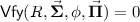), then $\mathsf {B}_\mathsf {alg}$ aborts. $(*)$ Otherwise $\mathsf {B}_\mathsf {alg}$ defines the univariate polynomial

$$ Q'_P(X):=Q_P(y_1X,\ldots ,y_5X). $$

If $Q'_P\equiv 0$ then $\mathsf {B}_\mathsf {alg}$ aborts. $(**)$ Otherwise $\mathsf {B}_\mathsf {alg}$ factors $Q'_P$ to obtain its roots (of which by (11) there are at most $(2n-1)^2$), checks them against its DLog instance to determine whether z is among them, and if so, returns z.

 

First note that $\mathsf {B}_\mathsf {alg}$ perfectly simulates for $\mathsf {A}_\mathsf {alg}$. Let us analyze the probability that $\mathsf {B}_\mathsf {alg}$ finds the target z provided that $\mathbf{bad } = 1$. In this case $\mathsf {B}_\mathsf {alg}$ will not abort at $(*)$.

Since $Q'_P(z)=Q_P(y_1z,\ldots ,y_5z) = Q_P(\vec x)$, by (15) we have $Q'_P(z) = 0$. Thus if $Q'_P\not \equiv 0$ then $\mathsf {B}_\mathsf {alg}$ finds z by factoring $Q'_P$. It remains to argue that $Q'_P\not \equiv 0$. By (15) we have $Q_P\not \equiv 0$. By the Schwartz-Zippel lemma, the probability that for a random , we have $Q_P(\vec y)=0$ is bounded by $\frac{d}{p-1}$ where d is the total degree of $Q_P$, which is bounded by $(2n-1)^2$. Since $Q_P(\vec y)=Q'_P(1)$, we have $Q'_P\not \equiv 0$ with probability at least $1-\frac{(2n-1)^2}{p-1}$. Since the choice of $\vec y$ is perfectly hidden from the adversary’s view this shows

where the last inequality comes from $n^2 \le (p-1)/8$. Putting this together with (13), we have shown that

Following the generic bound for Boneh and Boyen’s SDH assumption [BB08], we may assume that . The above equation thus implies

which concludes the proof.    $\square$

Corollary 6

It is $\big (\frac{3 t^2 q + 3 q^3}{p},t\big )$-hard to break knowledge soundness of Groth’s SNARK [Gro16] in the generic group model.

The corollary follows from the generic $\big (\frac{t^2 q + q^3}{p},t\big )$-hardness of , which is derived analogously to the bound for Boneh and Boyen’s SDH assumption [BB08].

We remark that the above result is not specific to Groth’s SNARK; it applies to any SNARK built from a NILP whose setup evaluates multivariate polynomials on a random position. The maximal total degree of these polynomials determines the parameter q in the q-DLog instance.

References

Abdalla, M., Benhamouda, F., MacKenzie, P.: Security of the J-PAKE password-authenticated key exchange protocol. In: 2015 IEEE Symposium on Security and Privacy, pp. 571–587. IEEE Computer Society Press, May 2015. 35
Abdalla, M., Bellare, M., Rogaway, P.: The oracle Diffie-Hellman assumptions and an analysis of DHIES. In: Naccache, D. (ed.) CT-RSA 2001. LNCS, vol. 2020, pp. 143–158. Springer, Heidelberg (2001). https://doi.org/10.1007/3-540-45353-9_12. 35, 45
Ambrona, M., Barthe, G., Schmidt, B.: Automated unbounded analysis of cryptographic constructions in the generic group model. In: Fischlin, M., Coron, J.-S. (eds.) EUROCRYPT 2016, Part II. LNCS, vol. 9666, pp. 822–851. Springer, Heidelberg (2016). https://doi.org/10.1007/978-3-662-49896-5_29. 39
Ateniese, G., Camenisch, J., de Medeiros, B.: Untraceable RFID tags via insubvertible encryption. In: Atluri, V., Meadows, C., Juels, A. (eds.) ACM CCS 2005, pp. 92–101. ACM Press, November 2005. 36
Ateniese, G., Camenisch, J., Hohenberger, S., de Medeiros, B.: Practical group signatures without random oracles. Cryptology ePrint Archive, Report 2005/385 (2005). http://eprint.iacr.org/2005/385. 36
Abe, M., Groth, J., Ohkubo, M.: Separating short structure-preserving signatures from non-interactive assumptions. In: Lee, D.H., Wang, X. (eds.) ASIACRYPT 2011. LNCS, vol. 7073, pp. 628–646. Springer, Heidelberg (2011). https://doi.org/10.1007/978-3-642-25385-0_34. 35
Aggarwal, D., Maurer, U.: Breaking RSA generically is equivalent to factoring. In: Joux, A. (ed.) EUROCRYPT 2009. LNCS, vol. 5479, pp. 36–53. Springer, Heidelberg (2009). https://doi.org/10.1007/978-3-642-01001-9_2. 34, 37
Boneh, D., Boyen, X.: Short signatures without random oracles and the SDH assumption in bilinear groups. J. Cryptol. 21(2), 149–177 (2008). 58
Bitansky, N., Chiesa, A., Ishai, Y., Paneth, O., Ostrovsky, R.: Succinct non-interactive arguments via linear interactive proofs. In: Sahai, A. (ed.) TCC 2013. LNCS, vol. 7785, pp. 315–333. Springer, Heidelberg (2013). https://doi.org/10.1007/978-3-642-36594-2_18. 52
Bangerter, E., Camenisch, J., Lysyanskaya, A.: A cryptographic framework for the controlled release of certified data. In: Security Protocols Workshop, pp. 20–24 (2004). 36
Bitansky, N., Canetti, R., Paneth, O., Rosen, A.: On the existence of extractable one-way functions. SIAM J. Comput. 45(5), 1910–1952 (2016). 38
Backes, M., Camenisch, J., Sommer, D.: Anonymous yet accountable access control. In: WPES, pp. 40–46 (2005). 36
Bao, F., Deng, R.H., Zhu, H.F.: Variations of Diffie-Hellman problem. In: Qing, S., Gollmann, D., Zhou, J. (eds.) ICICS 2003. LNCS, vol. 2836, pp. 301–312. Springer, Heidelberg (2003). https://doi.org/10.1007/978-3-540-39927-8_28. 43
Barthe, G., Fagerholm, E., Fiore, D., Mitchell, J.C., Scedrov, A., Schmidt, B.: Automated analysis of cryptographic assumptions in generic group models. In: Garay, J.A., Gennaro, R. (eds.) CRYPTO 2014, Part I. LNCS, vol. 8616, pp. 95–112. Springer, Heidelberg (2014). https://doi.org/10.1007/978-3-662-44371-2_6. 37, 39
Bernhard, D., Fischlin, M., Warinschi, B.: On the hardness of proving CCA-security of signed ElGamal. In: Cheng, C.-M., Chung, K.-M., Persiano, G., Yang, B.-Y. (eds.) PKC 2016, Part I. LNCS, vol. 9614, pp. 47–69. Springer, Heidelberg (2016). https://doi.org/10.1007/978-3-662-49384-7_3. 35
Brown, D.R.L., Gallant, R.P.: The static Diffie-Hellman problem. Cryptology ePrint Archive, Report 2004/306 (2004). http://eprint.iacr.org/2004/306. 37
Boneh, D., Lipton, R.J.: Algorithms for black-box fields and their application to cryptography (extended abstract). In: Koblitz, N. (ed.) CRYPTO 1996. LNCS, vol. 1109, pp. 283–297. Springer, Heidelberg (1996). https://doi.org/10.1007/3-540-68697-5_22. 33
Boneh, D., Lynn, B., Shacham, H.: Short signatures from the Weil pairing. J. Cryptol. 17(4), 297–319 (2004). 34, 48
Bresson, E., Monnerat, J., Vergnaud, D.: Separation results on the “one-more” computational problems. In: Malkin, T. (ed.) CT-RSA 2008. LNCS, vol. 4964, pp. 71–87. Springer, Heidelberg (2008). 35
Boyen, X.: The uber-assumption family (invited talk). In: Galbraith, S.D., Paterson, K.G. (eds.) Pairing 2008. LNCS, vol. 5209, pp. 39–56. Springer, Heidelberg (2008). https://doi.org/10.1007/978-3-540-85538-5_3. 38, 39
Bellare, M., Rogaway, P.: Random oracles are practical: a paradigm for designing efficient protocols. In: Ashby, V. (ed.) ACM CCS 1993, pp. 62–73. ACM Press, November 1993. 41
Bellare, M., Rogaway, P.: Code-based game-playing proofs and the security of triple encryption. Cryptology ePrint Archive, Report 2004/331 (2004). http://eprint.iacr.org/2004/331. 39
Boneh, D., Venkatesan, R.: Breaking RSA may not be equivalent to factoring. In: Nyberg, K. (ed.) EUROCRYPT 1998. LNCS, vol. 1403, pp. 59–71. Springer, Heidelberg (1998). https://doi.org/10.1007/BFb0054117. 34, 35, 40
Canetti, R., Goldreich, O., Halevi, S.: The random oracle methodology, revisited (preliminary version). In: 30th ACM STOC, pp. 209–218. ACM Press, May 1998. 38
Cheon, J.H.: Security analysis of the strong Diffie-Hellman problem. In: Vaudenay, S. (ed.) EUROCRYPT 2006. LNCS, vol. 4004, pp. 1–11. Springer, Heidelberg (2006). https://doi.org/10.1007/11761679_1. 37, 47
Camenisch, J., Hohenberger, S., Kohlweiss, M., Lysyanskaya, A., Meyerovich, M.: How to win the clonewars: efficient periodic n-times anonymous authentication. In: Juels, A., Wright, R.N., De Capitani di Vimercati, S. (eds.) ACM CCS 2006, pp. 201–210. ACM Press, October/November 2006. 36
Camenisch, J., Hohenberger, S., Lysyanskaya, A.: Compact e-cash. In: Cramer, R. (ed.) EUROCRYPT 2005. LNCS, vol. 3494, pp. 302–321. Springer, Heidelberg (2005). https://doi.org/10.1007/11426639_18. 36
Camenisch, J., Hohenberger, S., Pedersen, M.Ø.: Batch verification of short signatures. In: Naor, M. (ed.) EUROCRYPT 2007. LNCS, vol. 4515, pp. 246–263. Springer, Heidelberg (2007). https://doi.org/10.1007/978-3-540-72540-4_14. 36
Camenisch, J., Lysyanskaya, A.: Signature schemes and anonymous credentials from bilinear maps. In: Franklin, M. (ed.) CRYPTO 2004. LNCS, vol. 3152, pp. 56–72. Springer, Heidelberg (2004). https://doi.org/10.1007/978-3-540-28628-8_4. 35, 45
Chase, M., Meiklejohn, S.: Déjà Q: using dual systems to revisit q-type assumptions. In: Nguyen, P.Q., Oswald, E. (eds.) EUROCRYPT 2014. LNCS, vol. 8441, pp. 622–639. Springer, Heidelberg (2014). https://doi.org/10.1007/978-3-642-55220-5_34. 38
Coron, J.-S.: Optimal security proofs for PSS and other signature schemes. In: Knudsen, L.R. (ed.) EUROCRYPT 2002. LNCS, vol. 2332, pp. 272–287. Springer, Heidelberg (2002). https://doi.org/10.1007/3-540-46035-7_18. 35, 36
Damgård, I.: Towards practical public key systems secure against chosen ciphertext attacks. In: Feigenbaum, J. (ed.) CRYPTO 1991. LNCS, vol. 576, pp. 445–456. Springer, Heidelberg (1992). https://doi.org/10.1007/3-540-46766-1_36. 35, 38
Dent, A.W.: Adapting the weaknesses of the random oracle model to the generic group model. In: Zheng, Y. (ed.) ASIACRYPT 2002. LNCS, vol. 2501, pp. 100–109. Springer, Heidelberg (2002). https://doi.org/10.1007/3-540-36178-2_6. 38
Diffie, W., Hellman, M.E.: New directions in cryptography. IEEE Trans. Inf. Theory 22(6), 644–654 (1976). 35, 43
Garg, S., Bhaskar, R., Lokam, S.V.: Improved bounds on security reductions for discrete log based signatures. In: Wagner, D. (ed.) CRYPTO 2008. LNCS, vol. 5157, pp. 93–107. Springer, Heidelberg (2008). https://doi.org/10.1007/978-3-540-85174-5_6. 35
Ghadafi, E., Groth, J.: Towards a classification of non-interactive computational assumptions in cyclic groups. In: Takagi, T., Peyrin, T. (eds.) ASIACRYPT 2017. LNCS, vol. 10625, pp. 66–96. Springer, Cham (2017). https://doi.org/10.1007/978-3-319-70697-9_3. 38
Gennaro, R., Gentry, C., Parno, B., Raykova, M.: Quadratic span programs and succinct NIZKs without PCPs. In: Johansson, T., Nguyen, P.Q. (eds.) EUROCRYPT 2013. LNCS, vol. 7881, pp. 626–645. Springer, Heidelberg (2013). https://doi.org/10.1007/978-3-642-38348-9_37. 51
Groth, J.: On the size of pairing-based non-interactive arguments. In: Fischlin, M., Coron, J.-S. (eds.) EUROCRYPT 2016, Part II. LNCS, vol. 9666, pp. 305–326. Springer, Heidelberg (2016). https://doi.org/10.1007/978-3-662-49896-5_11. 36, 50, 52, 53, 54, 56, 58
Hellman, M.E., Pohlig, S.C.: An improved algorithm for computing logarithms over \({GF}(p)\) and its cryptographic significance. IEEE Trans. Inf. Theory 24(1), 106–110 (1978). 34
Jager, T., Rupp, A.: The semi-generic group model and applications to pairing-based cryptography. In: Abe, M. (ed.) ASIACRYPT 2010. LNCS, vol. 6477, pp. 539–556. Springer, Heidelberg (2010). https://doi.org/10.1007/978-3-642-17373-8_31. 34, 38
Joux, A., Rojat, A.: Security ranking among assumptions within the Uber Assumption framework. In: Desmedt, Y. (ed.) ISC 2013. LNCS, vol. 7807, pp. 391–406. Springer, Cham (2015). https://doi.org/10.1007/978-3-319-27659-5_28. 38
Jager, T., Schwenk, J.: On the analysis of cryptographic assumptions in the generic ring model. In: Matsui, M. (ed.) ASIACRYPT 2009. LNCS, vol. 5912, pp. 399–416. Springer, Heidelberg (2009). https://doi.org/10.1007/978-3-642-10366-7_24. 37
Kiltz, E.: A tool box of cryptographic functions related to the Diffie-Hellman function. In: Rangan, C.P., Ding, C. (eds.) INDOCRYPT 2001. LNCS, vol. 2247, pp. 339–349. Springer, Heidelberg (2001). https://doi.org/10.1007/3-540-45311-3_32. 38
Kakvi, S.A., Kiltz, E.: Optimal security proofs for full domain hash, revisited. In: Pointcheval, D., Johansson, T. (eds.) EUROCRYPT 2012. LNCS, vol. 7237, pp. 537–553. Springer, Heidelberg (2012). https://doi.org/10.1007/978-3-642-29011-4_32. 36
Kiltz, E., Masny, D., Pan, J.: Optimal security proofs for signatures from identification schemes. In: Robshaw, M., Katz, J. (eds.) CRYPTO 2016, Part II. LNCS, vol. 9815, pp. 33–61. Springer, Heidelberg (2016). https://doi.org/10.1007/978-3-662-53008-5_2. 35
Katz, J., Sahai, A., Waters, B.: Predicate encryption supporting disjunctions, polynomial equations, and inner products. In: Smart, N.P. (ed.) EUROCRYPT 2008. LNCS, vol. 4965, pp. 146–162. Springer, Heidelberg (2008). https://doi.org/10.1007/978-3-540-78967-3_9. 39
Leander, G., Rupp, A.: On the equivalence of RSA and factoring regarding generic ring algorithms. In: Lai, X., Chen, K. (eds.) ASIACRYPT 2006. LNCS, vol. 4284, pp. 241–251. Springer, Heidelberg (2006). https://doi.org/10.1007/11935230_16. 34
Lysyanskaya, A., Rivest, R.L., Sahai, A., Wolf, S.: Pseudonym systems. In: Heys, H.M., Adams, C.M. (eds.) SAC 1999. LNCS, vol. 1758, pp. 184–199. Springer, Heidelberg (2000). https://doi.org/10.1007/3-540-46513-8_14. 35, 37, 45
Maurer, U.M.: Abstract models of computation in cryptography (invited paper). In: Smart, N.P. (ed.) Cryptography and Coding 2005. LNCS, vol. 3796, pp. 1–12. Springer, Heidelberg (2005). https://doi.org/10.1007/11586821_1. 33, 37, 39, 42
Morillo, P., Ràfols, C., Villar, J.L.: The kernel matrix Diffie-Hellman assumption. In: Cheon, J.H., Takagi, T. (eds.) ASIACRYPT 2016, Part I. LNCS, vol. 10031, pp. 729–758. Springer, Heidelberg (2016). https://doi.org/10.1007/978-3-662-53887-6_27. 38
Maurer, U.M., Wolf, S.: Lower bounds on generic algorithms in groups. In: Nyberg, K. (ed.) EUROCRYPT 1998. LNCS, vol. 1403, pp. 72–84. Springer, Heidelberg (1998). https://doi.org/10.1007/BFb0054118. 33, 39
Maurer, U., Wolf, S.: The relationship between breaking the Diffie-Hellman protocol and computing discrete logarithms. SIAM J. Comput. 28(5), 1689–1721 (1999). 43
Nechaev, V.I.: Complexity of a determinate algorithm for the discrete logarithm. Math. Notes 55(2), 165–172 (1994). 33
Pollard, J.M.: Monte Carlo methods for index computation mod \(p\). Math. Comput. 32, 918–924 (1978). 34
Paillier, P., Vergnaud, D.: Discrete-log-based signatures may not be equivalent to discrete log. In: Roy, B.K. (ed.) ASIACRYPT 2005. LNCS, vol. 3788, pp. 1–20. Springer, Heidelberg (2005). 34, 35, 40
Rivest, R.L.: On the notion of pseudo-free groups. In: Naor, M. (ed.) TCC 2004. LNCS, vol. 2951, pp. 505–521. Springer, Heidelberg (2004). https://doi.org/10.1007/978-3-540-24638-1_28. 34
Rupp, A., Leander, G., Bangerter, E., Dent, A.W., Sadeghi, A.-R.: Sufficient conditions for intractability over black-box groups: generic lower bounds for generalized DL and DH problems. In: Pieprzyk, J. (ed.) ASIACRYPT 2008. LNCS, vol. 5350, pp. 489–505. Springer, Heidelberg (2008). https://doi.org/10.1007/978-3-540-89255-7_30. 39
Shoup, V.: Lower bounds for discrete logarithms and related problems. In: Fumy, W. (ed.) EUROCRYPT 1997. LNCS, vol. 1233, pp. 256–266. Springer, Heidelberg (1997). https://doi.org/10.1007/3-540-69053-0_18. 33, 37, 38, 39, 42
Shoup, V.: Sequences of games: a tool for taming complexity in security proofs. Cryptology ePrint Archive, Report 2004/332 (2004). http://eprint.iacr.org/2004/332
Sadeghi, A.-R., Steiner, M.: Assumptions related to discrete logarithms: why subtleties make a real difference. In: Pfitzmann, B. (ed.) EUROCRYPT 2001. LNCS, vol. 2045, pp. 244–261. Springer, Heidelberg (2001). https://doi.org/10.1007/3-540-44987-6_16. 38
Fuchsbauer, G., Kiltz, E., Loss, J.: The algebraic group model and its applications. Cryptology ePrint Archive, Report 2017/620 (2017). http://eprint.iacr.org/2004/332. 45, 47
Acknowledgments
We thank Dan Brown for valuable comments and Pooya Farshim for discussions on polynomials. We also thank Helger Lipmaa for sharing with us his independent security proof for Groth’s SNARK. The first author is supported by the French ANR EfTrEC project (ANR-16-CE39-0002). The second author was supported in part by ERC Project ERCC (FP7/615074) and by DFG SPP 1736 Big Data. The third author was supported by ERC Project ERCC (FP7/615074).
Author information
Authors and Affiliations
Corresponding author
Editor information
Editors and Affiliations
Rights and permissions
Copyright information
© 2018 International Association for Cryptologic Research
About this paper
Cite this paper
Fuchsbauer, G., Kiltz, E., Loss, J. (2018). The Algebraic Group Model and its Applications. In: Shacham, H., Boldyreva, A. (eds) Advances in Cryptology – CRYPTO 2018. CRYPTO 2018. Lecture Notes in Computer Science(), vol 10992. Springer, Cham. https://doi.org/10.1007/978-3-319-96881-0_2
Download citation
DOI: https://doi.org/10.1007/978-3-319-96881-0_2
Published:
Publisher Name: Springer, Cham
Print ISBN: 978-3-319-96880-3
Online ISBN: 978-3-319-96881-0
eBook Packages: Computer ScienceComputer Science (R0)