Focused and Synthetic Nested Sequents

Abstract

Focusing is a general technique for transforming a sequent proof system into one with a syntactic separation of non-deterministic choices without sacrificing completeness. This not only improves proof search, but also has the representational benefit of distilling sequent proofs into synthetic normal forms. We show how to apply the focusing technique to nested sequent calculi, a generalization of ordinary sequent calculi to tree-like instead of list-like structures. We thus improve the reach of focusing to the most commonly studied modal logics, the logics of the modal S5 cube. Among our key contributions is a focused cut-elimination theorem for focused nested sequents.

These keywords were added by machine and not by the authors. This process is experimental and the keywords may be updated as the learning algorithm improves.

1 Introduction

The focusing technique has its origin in the foundations of logic programming [1, 22] and is now increasingly relevant in structural proof theory because it improves proof search procedures [11, 21] and because focused proofs have clearly identifiable and semantically meaningful synthetic normal forms [6, 8, 10, 31]. The essential idea of focusing is to identify and coalesce the non-deterministic choices in a proof, so that a proof can be seen as an alternation of negative phases, where invertible rules are applied eagerly, and positive phases, where applications of the other rules are confined and controlled. This, in turn, lets us abstract from the usual unary and binary logical connectives by collapsing whole phases into n-ary synthetic connectives. The full theory of focusing was initially developed for the sequent calculus for linear logic [1], but it has since been extended to a wide variety of logics [11, 19, 27] and proof systems [4, 7]. This generality suggests that the ability to transform a proof system into a focused form is a good indication of its syntactic quality, in a manner similar to how admissibility of cut shows that a proof system is syntactically consistent.

It is natural to ask whether the focusing technique works as well for modal logics. Traditionally, modal logics are specified in terms of Hilbert-style axiomatic systems, but such systems are not particularly suitable since axioms reveal none of the structure of logical reasoning. It is well known that certain modal logics, $\mathsf {S5}$ in particular, are not representable in a variant of Gentzen’s sequent calculus without sacrificing analyticity. There are two principal ways to overcome this problem. The first is based on labeled proof systems that reify the Kripke semantics—the frame conditions—directly as formulas in the sequents [24, 29]. These “semantic formulas” are not subformulas of the end-sequent and they cause the interpretation of sequents to fall outside the class of propositional modal formulas, and for this reason, such calculi are also called external.

The second way is to use so-called internal calculi, that enrich the sequent structure such that analyticity is preserved and such that every sequent has an interpretation that stays inside the modal language. Well-known examples are hypersequents [2] and display calculi [3]. A more recent development are nested sequents [5, 12, 14, 26], which generalize the notion of context from a list-like structure (familiar from Gentzen’s sequent calculus) to a tree-like structure. Like ordinary sequents, nested sequents have a straightforward interpretation in the language of the logic, and enjoy cut admissibility (with a cut-elimination proof that stays wholly internal to the system) and hence the usual subformula property. Moreover, nested proof systems can be built modularly for every modal logic in the $\mathsf {S5}$ cube, in both classical and intuitionistic variants [5, 20].

In this paper, we build a focused variant, with its concomitant benefits, for all modal logics of the classical $\mathsf {S5}$ cube. For simplicity we use a polarized syntax [15] consisting of two classes of positive and negative formulas and a pair of shift connectives to move back and forth between the classes. Crucially, we interpret $\Diamond$ as positive and $\Box$ as negative, which differs from the polarity that would be assigned to these connectives if they were interpreted in terms of ? and !, respectively, from linear logic [25]. Our key technical contributions are: (1) a purely internal proof of cut-elimination for the focused nested calculus, given in terms of a traditional rewriting procedure to eliminate cuts (which shows that our system is compositional and suitably continuous), and (2) a proof of completeness of the focused system with respect to the non-focused system (and hence to the Kripke semantics) by showing that the focused system admits the rules of the non-focused system. It generalizes similar proofs of cut-elimination and focusing completeness for (non-nested) sequent calculi [11, 19].

To our knowledge there have been only two other attempts to apply the focusing technique to modal logics. The first uses a labeled system [23], using the work in [24] on geometric axioms to obtain systems that extend the basic modal logic $\mathsf {K}$. The cut-elimination and completeness results in [23] are obtained externally as a reduction to LKF, a focused system for first-order logic [19]. Therefore, the polarities of the modalities are inherited from the associated quantifiers, i.e., $\Box$ is negative and $\Diamond$ is positive, similar to our setting. The second approach [18] also uses nested sequents, but in a restricted form, in which the tree-structure is reduced to a single branch. This efficiently simulates the standard sequent system for the modal logic K, but makes both modalities positive.

Our approach uses the full power of nested sequents. and is intended as a prototype for how similar focused systems may be built for other modal logic formalisms. After some preliminaries (Sect. 2), we start with a weakly focused proof system (Sect. 3), where negative rules may be applied everywhere, including in the middle of focused phases. From this system, we extract a strongly focused system (also Sect. 3) and a synthetic system (Sect. 4) where the logical content of the phases of focusing are abstracted from the level of formulas to the level of nested sequents. We also sketch the cut-elimination theorem for this synthetic variant. The synthetic design generalizes similar designs for the sequent calculus [6, 31].

2 Modal Logics and the Nested Sequent Calculus $\mathsf {KN}$

Classical modal logic is obtained from classical propositional logic by adding the modal connectives $\Box$ and $\Diamond$. Starting with a countable set of atoms ($a, b, \ldots$), the formulas ($A, B, \ldots$) of modal logic are given by the following grammar:

$$\begin{aligned} A, B, ... \,{:}{:}{=}\,a \ | \bar{a} \ | \ A \wedge B \ | \ A \vee B \ |\ \Box A \ | \ \Diamond A \end{aligned}$$

(1)

To avoid excessive syntax, formulas are kept in negation-normal form, so the only formally negated formulas are the atoms. The negation $\bar{A}$ of an arbitrary formula A is given by the De Morgan laws: $\bar{\bar{A}}=A$, $\overline{A\wedge B}=\bar{A}\vee \bar{B}$ and $\overline{\Box A} = \Diamond \bar{A}$. We also define $A \supset B$ as $\bar{A} \vee B$, $A \equiv B$ as $(A \supset B) \wedge (B \supset A)$, $\top$ as $a \vee \bar{a}$, and $\bot$ as $a \wedge \bar{a}$ (for some atom a).

Modal logics are traditionally specified using Hilbert-style axiom schemata. The basic modal logic $\mathsf {K}$, for instance, is obtained by adding the following $\mathsf {k}$ axiom to the ordinary Hilbert axioms for propositional logic.

$$\begin{aligned} \mathsf {k}:\Box (A \supset B) \supset (\Box A \supset \Box B) \end{aligned}$$

(2)

To obtain the theorems of $\mathsf {K}$, we then also add two inference rules of modus ponens and necessitation.

$$\begin{aligned} \textsf {mp} \frac{{A} \ \ {A \supset B}}{B} \quad \quad \textsf {nec} \frac{A}{\Box A} \end{aligned}$$

(3)

Fig. 1.

Left: Some standard modal axioms          Right: Modal S5 cube

Stronger modal logics can be obtained by adding to $\mathsf {K}$ other axioms mentioning the modal connectives. In this paper, we consider the most common five axioms $\mathsf {d}$, $\mathsf {t}$, $\mathsf {b}$, $\mathsf {4}$ and $\mathsf {5}$, which are shown on the left in Fig. 1. Picking subsets of these axioms lets us define thirty-two modal logics, but only fifteen of them are non-redundant. For example, the sets $\{ {\mathsf {b}, \mathsf {4}} \}$ and $\{ {\mathsf {t}, \mathsf {5}} \}$ both yield the modal logic $\mathsf {S5}$. The fifteen distinct modal logics follow chains of extension from $\mathsf {K}$ to $\mathsf {S5}$ and can be arranged as a pair of nested cubes depicted on the right in Fig. 1; this is sometimes called the $\mathsf {S5}$ cube [13].

Fig. 2.

Rules for . The first row constitutes $\mathsf {KN}$.

Let us recall the notion of nested sequents, first defined by Kashima [14] and then independently rediscovered by Poggiolesi [26] (who called them tree-hypersequents) and Brünnler [5]. In Gentzen’s one-sided sequent calculus, a sequent is just a multiset of formulas; nested sequents generalize this notion to a multiset of formulas and boxed sequents, resulting in a tree structure.

Definition 2.1

A nested sequent ($\varGamma ,\varDelta ,\ldots$) is a finite multiset of formulas and boxed sequents of the form $[\varDelta ]$, where $\varDelta$ is itself a nested sequent. In other words, nested sequents have the following grammar:

$$\begin{aligned} \varGamma , \varDelta , \ldots \,{:}{:}{=}\,A_1, \ldots , A_m, [\varGamma _1], \ldots , [\varGamma _n] \end{aligned}$$

(4)

Both m and n may be 0, in which case the sequent is empty; when we need to be explicit, we will use the notation $\emptyset$ to stand for an empty sequent. As is usual in sequent calculi, we consider the comma to be associative and commutative.

Definition 2.2

(Corresponding Formulas). For any nested sequent $\varGamma$, a corresponding formula, written $\mathrm {fm}(\varGamma )$, gives an interpretation of $\varGamma$ as a modal logic formula. Corresponding formulas obey the following equivalences: $\mathrm {fm}(\emptyset ) \equiv \bot$, $\mathrm {fm}(A) \equiv A$, $\mathrm {fm}([\varGamma ]) \equiv \Box \mathrm {fm}(\varGamma )$, and $\mathrm {fm}(\varGamma _1, \varGamma _2) \equiv \mathrm {fm}(\varGamma _1) \vee \mathrm {fm}(\varGamma _2)$.

Definition 2.3

(Context). An n-holed context is like a nested sequent but contains n pairwise distinct numbered holes of the form $\{\}_i$ (for $1 \le i \le n$) in place of formulas. (No hole can occur inside a formula.) We depict such a context as $\varGamma \{\}_1\cdots \{\}_n$. Given such a context and n nested sequents $\varDelta _1, \ldots , \varDelta _n$, we write $\varGamma \{\varDelta _1\}_1\cdots \{\varDelta _n\}_n$ to stand for the nested sequent where the hole $\{\}_i$ (for $1 \le i \le n$) in the context has been replaced by $\varDelta _i$, with the understanding that if $\varDelta _i$ is empty then the hole is simply removed. Unless there is any ambiguity, we will omit the hole index subscripts in this paper to keep the notation light.

Definition 2.4

The depth of $\varGamma \{\}$, written $\mathrm {dp}(\varGamma \{\})$, is given inductively by: $\mathrm {dp}(\{\}) = 0$, $\mathrm {dp}(\varDelta , \varGamma \{\}) = \mathrm {dp}(\varGamma \{\})$, and $\mathrm {dp}([\varGamma \{\}]) = \mathrm {dp}(\varGamma \{\}) + 1$.

Example 2.5

Let $\varGamma \{\}\{\} = A, [B, \{ {} \}, [\{ {} \}], C]$. For the sequents $\varDelta _1 = D$ and $\varDelta _2 = A, [C]$, we get: $\varGamma \{\varDelta _1\}\{\varDelta _2\} = A, [B, D , [A, [C]], C]$ and $\varGamma \{\emptyset \}\{\varDelta _2\} = A, [B, [A, [C]], C]$. We also have that $\mathrm {dp}(\varGamma \{\}\{\varDelta _1\}) = 1$ and $\mathrm {dp}(\varGamma \{\varDelta _1\}\{\ \})=2$.

The basic modal logic $\mathsf {K}$ (as presented in [5]) is captured using nested sequents as the cut-free proof system $\mathsf {KN}$ shown in the first row in Fig. 2. The deductive system corresponding to each normal extension $\mathsf {K}+ \mathsf {X}$, where $\mathsf {X}\subseteq \{ {\mathsf {d}, \mathsf {t}, \mathsf {b}, \mathsf {4}, \mathsf {5}} \}$ is a set of modal axioms (Fig. 1), can be obtained by adding the corresponding diamond rules (final two rows of Fig. 2) to $\mathsf {KN}$. The rule has a side condition that the context in which the principal $\Diamond$-formula occurs has non-zero depth, i.e., that it does not occur at the root of the conclusion sequent.

To make the correspondence between extensions of $\mathsf {K}$ and the proof systems precise, we need the following additional notion:

Definition 2.6

(45-Closure). We say that $\mathsf {X}\subseteq \{ {\mathsf {d}, \mathsf {t}, \mathsf {b}, \mathsf {4}, \mathsf {5}} \}$ is 45-closed, if:

• whenever $\mathsf {4}$ is derivable in $\mathsf {K}+ \mathsf {X}$, $\mathsf {4}\in \mathsf {X}$

• whenever $\mathsf {5}$ is derivable in $\mathsf {K}+ \mathsf {X}$, $\mathsf {5}\in \mathsf {X}$.

In this paper, we will always work with 45-closed axiom sets. The reason is that, for example, the axiom $\mathsf {4}$ is not provable (without cut) in even though $\mathsf {4}$ is a theorem of the logic $\mathsf {K}+\{ {\mathsf {t},\mathsf {5}} \}$ (which is $\mathsf {S5}$). Note that this is not a real restriction, since for every logic in the modal cube (Fig. 1) there is a 45-closed set of axioms defining it (see [5] for details). We can now state the soundness, completeness, and cut-admissibility for $\mathsf {KN}$ and its extensions.

Theorem 2.7

Let $\mathsf {cut}$ be the following rule:

$$\begin{aligned} \mathsf {cut}\frac{\varGamma \{A\} \ \ \varGamma \{\bar{A}\}}{\varGamma \{\emptyset \}} \end{aligned}$$

Let $\mathsf {X}\subseteq \{ {\mathsf {d}, \mathsf {t}, \mathsf {b}, \mathsf {4}, \mathsf {5}} \}$ be 45-closed. For any formula A, the following are equivalent.

• 1. A is a theorem of $\mathsf {K}+\mathsf {X}$.

• 2. A is provable in .

• 3. A is provable in .

The proof that $1\Longrightarrow 2\Longrightarrow 3\Longrightarrow 1$ can be found in [5].    $\square$

3 The Focused Systems $\mathsf {KNwF}$ and $\mathsf {KNF}$

The essence of the focusing technique [1] is to classify formulas into positive formulas, whose rules are not invertible, and negative whose rules are invertible. (As usual, we consider a rule to be invertible if whenever the conclusion of the rule is derivable then so are each of its premises.) Due to invertibility, when searching for a proof it is always safe to apply—reading from conclusion to premises—a rule for a negative formula, so these may be applied at any time. On the other hand, rules for positive formulas may require rules on other formulas to be applied first. For example, the $\mathsf {KN}$ sequent $\Box \bar{a}, \Diamond a$ can only be proved by first applying the $\Box$ rule, showing that $\Diamond$-formulas are positive. A focused proof is one where the decision to apply a rule to a positive formula has to be explicitly taken, which then commits the proof to continue applying rules to this focused positive formula and its immediate positive descendants (and no other formula in the sequent), which drastically reduces the search space. The main theorem of focusing is that this strategy is complete, i.e., every theorem has a focused proof.

We will now build such a focused version of $\mathsf {KN}$. To simplify the meta-theorems about this system, we will adopt a polarized syntax [15] where the positive and negative formulas are grouped together in different syntactic categories and explicitly mediated by shift connectives ($\uparrow$ and $\downarrow$). As already mentioned, $\Diamond$ is in the positive class, and its dual $\Box$ is in the negative class, unlike what would be expected if they were interpreted in terms of the linear logic modalities ? and ! respectively. One way of explaining this phenomenon is that the standard shallow rule $\mathsf k$ in sequent calculus (corresponding to the promotion rule of linear logic) realises two steps at once: accessing the formula under a $\Box$ and moving the $\Diamond$-formulas from the context next to that formula. These two steps are done by two different rules $\Box$ and in nested sequent systems like $\mathsf {KN}$.

The rest of the formulas have ambiguous polarities and the choice does not alter the focusing result — some reasons to pick certain polarizations can be found in [11, 19]. We arbitrarily assign all atoms to be positive (and their negations to be negative), and present the system in the strongest form, i.e., split the conjunctions and disjunctions into positive and negative versions. Thus, polarized formulas have the following grammar:

(5)

Each column in the grammar above defines a De Morgan dual pair; note that the negation of a positive formula is a negative formula, and vice versa. Units are definable similarly to the non-focused case, so we have , and dually for $f^-$/$t^-$. When the polarity of a formula is not important, we write it as $A, B, \ldots$. A polarized nested sequent is the same as in the non-focused setting, with the difference that all formulas are polarized. Likewise, a polarized context is a polarized nested sequent where some formulas have been replaced by holes. In the rest of this paper, we will drop the adjective “polarized” and treat all constructs implicitly as polarized, unless otherwise indicated.

Definition 3.1

(Neutral). A formula is said to be neutral if it is a positive formula or a negated atom. A nested sequent is neutral if it is built from multisets of neutral formulas and boxed neutral sequents. A context $\varGamma \{\}\cdots \{\}$ is neutral if $\varGamma \{\emptyset \}\cdots \{\emptyset \}$ is neutral.

Definition 3.2

A focused sequent is of the form $\varGamma \{{\left\langle {P} \right\rangle }\}$ where $\varGamma \{\}$ is a context and P is a positive formula. The formula P is called its focus. The notion of corresponding formula (Definition 2.2) is extended with $\mathrm {fm}({\left\langle {P} \right\rangle }) \equiv \mathrm {fm}(P)$.

Fig. 3.

Focused Rules for and . The first three rows constitute $\mathsf {KNwF}$ and $\mathsf {KNF}$.

The inference rules of the focused system $\mathsf {KNwF}$ ($\mathsf {w}$ for “weak”) are shown in the first three rows in Fig. 3 (the basic system for $\mathsf {K}$). Then, for a set $\mathsf {X}\subseteq \{ {\mathsf {d}, \mathsf {t}, \mathsf {b}, \mathsf {4}, \mathsf {5}} \}$, we write for the corresponding subset of the focused diamond rules in the last two rows. Observe that the rules for negative formulas are exactly the same as in the unfocused system, while the rules for positive formulas can only be applied if the principal formula is in focus. Mediating between ordinary and focused sequents are the rules $\mathsf {dec}$ (“decide”), that chooses a positive formula in the conclusion and focuses on a copy of it in the premise, and $\mathsf {rel}$ (“release”) that drops the focus on a shifted formula. Since $\mathsf {dec}$ keeps the original positive formula in the context, there is no need to incorporate contraction in every positive rule, like in $\mathsf {KN}$. The $\mathsf {sto}$ (“store”) rule removes a shift in front of a positive formula and is used to produce neutral premises from non-neutral conclusions.

We define the system $\mathsf {KNF}$ to be a restriction of $\mathsf {KNwF}$ where the conclusion of the $\mathsf {dec}$ rule is required to be neutral, as well as the contexts surrounding the focus in all rules involving focused sequents. Thus, in $\mathsf {KNF}$, the $\mathsf {dec}$ rule is only applicable when no other rule is applicable (no negative rule as there is no negative formula in a neutral sequent and no positive rule as there is no focus), and hence we sometimes call it strongly focused. We immediately have the following proposition:

Proposition 3.3

Let $X\subseteq \{ {\mathsf {d}, \mathsf {t}, \mathsf {b}, \mathsf {4}, \mathsf {5}} \}$. A formula A is provable in if and only if it is provable in .

Proof

A derivation in is by definition also a derivation in . Conversely, to convert a derivation in into one in , we first have to replace all instances of $\mathsf {id}$ with a sequence of applications of followed (reading from conclusion upwards) by $\mathsf {id}$, to ensure that the conclusion of the $\mathsf {id}$ rule is neutral. Then, the negative rules can be permuted down by straightforward rule permutations to ensure that $\mathsf {dec}$ only applies to neutral sequents.    $\square$

In order to establish the soundness and completeness of $\mathsf {KNwF}$, we use the obvious forgetful injection of the polarized syntax into the unpolarized syntax.

Definition 3.4

(Depolarization). If A is a polarized formula, then we write $\lfloor A \rfloor$ for the unpolarized formula obtained from A by erasing the shifts $\mathord \uparrow$ and $\mathord \downarrow$, collapsing and into $\wedge$, and collapsing and into $\vee$.

Theorem 3.5

(Soundness). Let $X\subseteq \{ {\mathsf {d}, \mathsf {t}, \mathsf {b}, \mathsf {4}, \mathsf {5}} \}$. If a formula A is provable in , then $\lfloor A \rfloor$ is provable in .

Proof

By forgetting the polarity information, every proof of A is transformed into a proof of $\lfloor A \rfloor$.    $\square$

Completeness is considerably trickier. We use a technique pioneered by Laurent for linear logic [16] and proceed via cut-elimination in $\mathsf {KNwF}$.

Fig. 4.

Structural rules.

Fig. 5.

Structural modal rules for axioms $\mathsf {d}, \mathsf {t}, \mathsf {b}, \mathsf {4}, \mathsf {5}$ (where $\mathrm {dp}(\varGamma \{\ \}\{[\varDelta ]\}) \ge 1$ in )

3.1 Cut Elimination

In this section we will show that a collection of cuts is admissible for . As usual, a rule is said to be admissible if it is the case that whenever any instance of all its premises is derivable, so is the corresponding instance of the conclusion. In order to show the admissibility of the cut rules, it will be very useful to appeal to a collection of other admissible and invertible rules.

Lemma 3.6

Let $\mathsf {X}\subseteq \{ {\mathsf {d}, \mathsf {t}, \mathsf {b}, \mathsf {4}, \mathsf {5}} \}$. The rules $\mathsf {weak}$, $\mathsf {weak}_{\mathsf {f}}$, $\mathsf {cont}$, and (shown in Fig. 4) are admissible for . Moreover, the rules $\mathsf {sto}$, $\Box$, , and are invertible for .

Proof

By straightforward induction on the height of the derivation.    $\square$

Note that here we use contraction only on negated atoms because that is all that is needed in the cut-elimination proof below. One can indeed show that the general contraction rule on arbitrary sequents (and not just formulas) is admissible, but this requires a complicated argument for focused sequents. The corresponding result for $\mathsf {KN}$ is shown in [5].

Lemma 3.7

Let $\mathsf {X}\subseteq \{ {\mathsf {d}, \mathsf {t}, \mathsf {b}, \mathsf {4}, \mathsf {5}} \}$. If $\mathsf {X}$ is 45-closed, then any rule in (shown in Fig. 5) is admissible for .

Proof

Analogous to the corresponding lemma for $\mathsf {KN}$ in [5, Lemma 9]. The full proof can be found in [9, Lemma 3.7].    $\square$

Fig. 6.

The various cuts in

We are now ready to prove the admissibility of cuts. Specifically, we show all the cuts in Fig. 6 are simultaneously admissible. The $\mathsf {cut}_1$ rule is our standard cut between ordinary nested sequents, while $\mathsf {cut}_2$ defines a principal cut between a focus and its dual as cut formulas. Finally, $\mathsf {cut}_3$ is a commutative cut for situations where the positive cut formula is not principal. Note that this collection of cuts is just sufficiently large to make the standard cuts admissible. It is easy to imagine many other cut-like rules, but it is not necessary—and may not even be possible—to admit them.

Definition 3.8

The height of a formula A, written $\mathrm {ht}(A)$, is computed inductively as follows: $\mathrm {ht}(a)=\mathrm {ht}(\bar{a})=1$, $\mathrm {ht}(A\star B)=\max (\mathrm {ht}(A),\mathrm {ht}(B))+1$ where , and $\mathrm {ht}(\bigcirc A)= \mathrm {ht}(A)+1$ where $\bigcirc \in \{ {\Diamond ,\Box ,\mathord \uparrow ,\mathord \downarrow } \}$. The rank of an instance of one of the cut rules is the height of its cut formula (the P in Fig. 6).

Lemma 3.9

(Cut Reduction). Let $\mathsf {X}\subseteq \{ {\mathsf {d}, \mathsf {t}, \mathsf {b}, \mathsf {4}, \mathsf {5}} \}$ be 45-closed. For every derivation

(6)

in , where $\mathcal {D}_1$ and $\mathcal {D}_2$ are cut-free, there is a cut-free derivation of $\varGamma _0$ in .

Proof

Let $\mathcal {D}_1$ always stand for the derivation with the positive cut formula. We proceed by lexicographic induction: the induction hypothesis may be applied whenever (1) the rank of the cut decreases, or (2) the rank stays the same and a $\mathsf {cut}_1$ is replaced by a $\mathsf {cut}_2$, or (3) the rank stays the same and the height of $\mathcal {D}_1$ decreases. The height of $\mathcal {D}_2$ does not matter for the induction. The proof is then given in terms of a terminating rewrite sequence, written with .

Most cases of this rewrite are standard, so we show here only certain cases characteristic of focusing; the full list of cases can be found in [9, Lemma 3.9].

• The commutative cases are simple, relying on the invertibility of the negative rules (Lemma 3.7). Here we show the case of $\mathsf {rel}$ above a $\mathsf {cut}_3$:

  

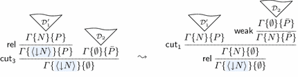
  The resulting $\mathsf {cut}_2$ can be reduced because it has a smaller height.

• The cases of $\mathsf {dec}$ with the cut formula being principal:

  

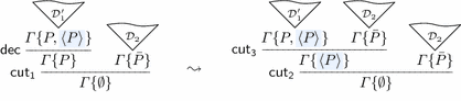
  In the resulting derivation, we first reduce the upper $\mathsf {cut}_3$, which is allowed because the height is smaller. Then, we reduce the lower cut, which is allowed because a $\mathsf {cut}_2$ can be used to justify a $\mathsf {cut}_1$ of the same rank.

• Finally, here is a characteristic case for the modal axioms, for the rule: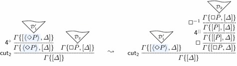

  

  The resulting $\mathsf {cut}_2$ can be reduced because it has a smaller height. In the right branch, the ${\Box }^{-1}$ rule is the admissible inverse of the $\Box$ rule (Lemma 3.6) and the rule is given by Lemma 3.7.    $\square$

Theorem 3.10

Let $\mathsf {X}\subseteq \{ {\mathsf {d}, \mathsf {t}, \mathsf {b}, \mathsf {4}, \mathsf {5}} \}$ be 45-closed. If a sequent $\varGamma$ is provable in , then it is also provable in .

Proof

Apply Lemma 3.9 to all cut instances in the derivation, starting with a topmost one. This gives us a cut-free proof in , from which we get a cut-free proof in using Proposition 3.3.    $\square$

3.2 Completeness

We can now use Theorem 3.10 to show completeness of the focused systems (and hence ) with respect to . As an intermediate step, we consider a variant of $\mathsf {KN}$ that can deal with polarized formulas. Let $\mathsf {KN'}$ denote the system that is obtained from $\mathsf {KN}$ by adding the rules

$$\mathsf {rel}\frac{\varGamma \{N\}}{\varGamma \{\mathord \downarrow N\}} \quad \quad \mathsf {sto}\frac{\varGamma \{P\}}{\varGamma \{\mathord \uparrow P\}}$$

and by duplicating the rules for $\wedge$ and $\vee$ such that there is a variant for each of and , and and , respectively. We immediately have the following lemma:

Lemma 3.11

A formula A is provable in if and only if $\lfloor A \rfloor$ is provable in .    $\square$

We are now going to simulate in . For this, we need another property of $\mathsf {KNwF}$:

Lemma 3.12

(Identity Reduction). The following rule is derivable in $\mathsf {KNwF}$:

Proof

By straightforward induction on the height of P. Details can be found in [9, Lemma 3.12].    $\square$

Lemma 3.13

(Simulation). Let $\mathsf {X}\subseteq \{ {\mathsf {d}, \mathsf {t}, \mathsf {b}, \mathsf {4}, \mathsf {5}} \}$ and let A be a formula that is provable in . Then A is provable in .

Proof

We show that each rule in is derivable in . Then the lemma follows by replacing in the proof of A in each instance of a rule by the corresponding derivation in . For the rules this is trivial. We show below the cases for , , and . The others are similar, and a full list can be found in [9, Lemma 3.13].

Note that we make a crucial use of $\mathsf {cut_1}$ and Lemma 3.12.    $\square$

Theorem 3.14

(Completeness). Let $\mathsf {X}\subseteq \{ {\mathsf {d}, \mathsf {t}, \mathsf {b}, \mathsf {4}, \mathsf {5}} \}$ be 45-closed. For any A, if $\lfloor A \rfloor$ is provable in , then A is provable in .

Proof

Suppose that we have a proof of $\lfloor A \rfloor$ in . By Lemma 3.11, there is a proof of A in . Then, by Lemma 3.13, there is also a proof of A in . Finally, using Theorem 3.10, we get a proof in .    $\square$

4 The Synthetic System

As already mentioned, the strongly focused system $\mathsf {KNF}$ is given as a restriction of $\mathsf {KNwF}$ where the $\mathsf {dec}$ rule is restricted to neutral contexts. However, the cut-elimination and admissibility theorems (3.9 and 3.10) were proved in the $\mathsf {KNwF}$ system and made essential use of the admissibility of weakening by arbitrary formulas, including negative formulas, and of the possibility of applying negative rules even within a positive phase. This freedom simplifies the proofs of the meta-theorems, and leaves them at least a recognizable variant of similar proofs in the non-focused system $\mathsf {KN}$. Of course, thanks to Proposition 3.3, we also have a cut-elimination proof for , but this is not entirely satisfactory: it is not an internal proof, i.e., a sequence of cut reductions for that stays inside the system.

One possible response to this issue might be to try to redo the cut-elimination using just , but this quickly gets rather complicated because we no longer have access to the weakening rules (Fig. 4) in the case where the weakened structure contains negative formulas. Indeed, published proofs of similar attempts for the sequent calculus usually solve this problem by adding additional cut rules, which greatly complicates the cut-elimination argument [11, 19, 28].

Fig. 7.

Synthetic substructure matching

To avoid this complexity, it is better to consider the focused proof system in a synthetic form where the logical inference rules for the various connectives are composed as much as possible, so that the proof system itself contains exactly two logical rules: one for a positive and one for a negative synthetic connective [6, 31]. This synthetic view moreover improves the concept of focusing itself by showing that a focused proof consists of: (1) a selection of a certain substructure (the generalization of subformula) of the principal formula, and (2) the contextualization of that substructure. For positive principal formulas, this contextualization is in the form of a check in the surrounding context for other structures, such as dual atoms or nested sequents. For negative principal formulas, on the other hand, contextualization amounts to asserting the presence of additional structure in the surrounding context. This design will become clear in the explicit formulation of the synthetic version of $\mathsf {KNF}$—which we call $\mathsf {KNS}$—in the rest of this section.

4.1 Synthetic Substructures

For any negative formula, there is a collection of corresponding nested sequents that represents one of the possible branches taken in a sequence of negative rules applied to the formula. This correspondence is formally given below.

Definition 4.1

(Matching). The nested sequence $\varGamma$ matches the negative formula N, written $\varGamma \preccurlyeq N$, if it is derivable from the rules in Fig. 7.

For the system to follow, we will use two additional sequent-like structures that are not themselves neutral sequents.

Definition 4.2

(Extended Sequents)

• An inversion sequent is a structure of the form $\varGamma \{N\}$ where $\varGamma \{\}$ is a neutral sequent context.

• A focused sequent is a structure of the form $\varGamma \{{\left\langle {\varDelta } \right\rangle }\}$ where $\varGamma \{\}$ is a neutral sequent context and $\varDelta$ is a neutral sequent.

Note that in $\varGamma \{N\}$, there is exactly one occurrence of N as a top-level formula anywhere; likewise, in $\varGamma \{{\left\langle {\varDelta } \right\rangle }\}$, there is a single occurrence of the sub-structure ${\left\langle {\varDelta } \right\rangle }$. Hence, these extended sequent forms uniquely determine their decomposition into context (the $\varGamma \{\}$) and the extended entity (the N or the ${\left\langle {\varDelta } \right\rangle }$).

Definition 4.3

(Corresponding Formula). A corresponding formula of a neutral or extended sequent $\varGamma$, denoted as $\mathrm {f\bar{m}}(\varGamma )$, is a negative formula satisfying:

where $N \equiv M$ stands for .

Fig. 8.

Synthetic rules for ${\mathsf {KNS}}+{\mathsf {X}^{\left\langle {} \right\rangle }}$. The first two rows constitute $\mathsf {KNS}$.

The system $\mathsf {KNS}$ consists of the rules in the first two lines of Fig. 8. For a set $\mathsf {X}\subseteq \{ {\mathsf {d}, \mathsf {t}, \mathsf {b}, \mathsf {4}, \mathsf {5}} \}$, we write $\mathsf {X}^{\left\langle {} \right\rangle }\subseteq \{ {\mathsf {d}^{\left\langle {} \right\rangle },\mathsf {t}^{\left\langle {} \right\rangle },\mathsf {b}^{\left\langle {} \right\rangle },\mathsf {4}^{\left\langle {} \right\rangle },\mathsf {5}^{\left\langle {} \right\rangle }} \}$ for the corresponding structural rules in Fig. 8, and ${\mathsf {KNS}}+{\mathsf {X}^{\left\langle {} \right\rangle }}$ for the corresponding system. It becomes clearer that the duality between positive and negative synthetic rules amounts to a meta-quantification over substructures: the positive rule $\mathsf {pos}^{\left\langle {} \right\rangle }$ quantifies existentially over the substructures of $\bar{P}$ and pick one such $\varDelta$ as a focus in the unique premise, while the negative rule quantifies universally, and so the rule actually consists of one premise for each way in which to prove $\varDelta \preccurlyeq N$. Thus, for example, if N is , then we know that $\bar{a} \preccurlyeq N$ and $[\bar{b}, P] \preccurlyeq N$, so the rule instance in this case is:

It is instructive to compare with (and hence also ). In the latter system, the focus is used to drive the modal rules . Such modal rules can be applied only a fixed number of times before needs to be reduced to , and logical rules or the identity to be used — which is necessary to finish the proof since foci can never be weakened. Thus, the analysis of P is forced to be interleaved with the modal rules for , as shown by the alternation of and in the derivation on the left below. In , in contrast, the rule itself performs the analysis of P up front to produce a synthetic substructure; the modal rules then work entirely at the level of focused substructures, as in the derivation on the right below.

Thus, the modal rules of are properly seen as structural rules rather than logical rules.

4.2 Cut Elimination

Cut elimination for is achieved in a similar way to that for .

Lemma 4.4

(Admissible Rules). The rules $\mathsf {weak}$, $\mathsf {weak}_{\mathsf {f}}$, $\mathsf {cont}$, (shown in Fig. 4), restricted to neutral and extended sequents (as appropriate) are admissible in . Moreover, if $\mathsf {X}\subseteq \{ {\mathsf {d}, \mathsf {t}, \mathsf {b}, \mathsf {4}, \mathsf {5}} \}$ is 45-closed, then any rule (see Fig. 5) is admissible in ${\mathsf {KNS}}+{\mathsf {X}^{\left\langle {} \right\rangle }}$.

Proof

By induction on the height of the derivation, analogous to the proofs of Lemmas 3.6 and 3.7.    $\square$

Note that we do not allow, e.g., weakening $\varGamma \{{\left\langle {\varDelta } \right\rangle }\}\{\emptyset \}$ to $\varGamma \{{\left\langle {\varDelta } \right\rangle }\}\{N\}$; the latter is, in fact, not even a well-formed $\mathsf {KNS}$ focused sequent. Like with $\mathsf {KNwF}$, we have three cut rules for $\mathsf {KNS}$, which are shown in Fig. 9. We can now give the synthetic variant of the cut-elimination theorem.

Fig. 9.

Synthetic variants of the cut rule (cf. Fig. 6)

Theorem 4.5

Let $\mathsf {X}\subseteq \{ {\mathsf {d}, \mathsf {t}, \mathsf {b}, \mathsf {4}, \mathsf {5}} \}$ be 45-closed. Each rule of $\{ {\mathsf {cut}^{\left\langle {} \right\rangle }_1, \mathsf {cut}^{\left\langle {} \right\rangle }_2, \mathsf {cut}^{\left\langle {} \right\rangle }_3} \}$ is admissible in ${\mathsf {KNS}}+{\mathsf {X}^{\left\langle {} \right\rangle }}$.

Proof

The idea of the proof is similar to that of Theorem 3.10, using a reduction similar to that of Lemma 3.9. However, in the synthetic case there is a complication because the inverse of the negative rule $\mathsf {neg}^{\left\langle {} \right\rangle }$ is not admissible in . The cut reduction argument therefore has to work at the level of synthetic derivations. We show two illustrative examples here. The first is the case where the cut formula is principal in both derivations:

The instance of $\mathsf {cut}^{\left\langle {} \right\rangle }_3$ can be reduced because the height is smaller, while that of $\mathsf {cut}^{\left\langle {} \right\rangle }_2$ can be reduced because a $\mathsf {cut}^{\left\langle {} \right\rangle }_2$ can justify a $\mathsf {cut}^{\left\langle {} \right\rangle }_1$ of the same rank. The other illustrative case is for permuting a $\mathsf {cut}^{\left\langle {} \right\rangle }_3$ past a $\mathsf {rel}^{\left\langle {} \right\rangle }$.

The instance of $\mathsf {weak}$ is justified by Lemma 4.4. The remainder of the cases of the proof have to be adjusted similarly. The full proof can be found in [9, Theorem 4.5].    $\square$

It is worth remarking that this cut-elimination proof did not have to mention any logical connectives, and was instead able to factorize all logical reasoning in terms of the matching. This means that the matching judgement can be modified at will without affecting the nature of the cut argument, as long as it leaves the structure of nested sequents untouched. This makes our result modular in yet another way, in addition to the modularity obtained by means of the structural rules for foci. Indeed, we can obtain a similarly synthetic version of identity reduction (Lemma 3.12).

Lemma 4.6

(Identity Reduction). The following rule is derivable in $\mathsf {KNS}$.

Proof

By induction on the structure of the focus, ${\left\langle {\varDelta } \right\rangle }$. The full proof can be found in [9, Lemma 4.6].    $\square$

Showing sound and complete with respect to is fairly straightforward and the details are omitted here. Soundness follows directly from replacing the $\mathsf {KNS}$ sequent $\varGamma \{{\left\langle {\varDelta } \right\rangle }\}$ with the $\mathsf {KNF}$ sequent $\varGamma \{{\left\langle {\overline{\mathrm {f\bar{m}}(\varDelta )}} \right\rangle }\}$ and then interpreting the proof in , using matching derivation (Fig. 7) to determine how to choose between the two rules. For completeness, we can follow the strategy of Lemma 3.13 nearly unchanged. However, like with the cut-elimination proof, we have to avoid appeals to weakening with negative formulas by using the synthetic form of $\mathsf {neg}^{\left\langle {} \right\rangle }$.

5 Perspectives

We have presented strongly focused and synthetic systems for all modal logics in the classical $\mathsf {S5}$-cube. We used the formalism of nested sequents as carrier, but we are confident that something similar can be achieved for hypersequents, for example based on the work of Lellmann [17]. We chose nested sequents over hypersequents for two reasons. First, the formula interpretation of a nested sequent is the same for all logics in the $\mathsf {S5}$-cube, which simplifies the presentation of the meta-theory. Second, due to the close correspondence between nested sequents and prefixed tableaux [12] we can from our work directly extract focused tableau systems for modal logics. Furthermore, even though we spoke in this paper only about classical modal logic, we are confident that the same results can also be obtained for the intuitionistic variant of the modal $\mathsf {S5}$-cube [29], if we start from the non-focused systems in [30].

One extension that would be worth considering would be relaxing the restriction that there can be at most one focus in a $\mathsf {KNF}$ or $\mathsf {KNS}$ proof. Allowing multiple foci would take us from ordinary focusing to multi-focusing, which is well known to reveal more parallelism in sequent proofs [10]. It has been shown that a certain well chosen multi-focusing system can yield syntactically canonical representatives of equivalence classes of sequent proofs for classical predicate logic [8]. Extending this approach to the modal case seems promising.

References

Andreoli, J.-M.: Logic programming with focusing proofs in linear logic. J. Logic Comput. 2(3), 297–347 (1992)
Avron, A.: The method of hypersequents in the proof theory of propositional non-classical logics. In: Logic: From Foundations to Applications: European Logic Colloquium, pp. 1–32. Clarendon Press (1996)
Belnap Jr., N.D.: Display logic. J. Philos. Logic 11, 375–417 (1982)
Brock-Nannestad, T., Schürmann, C.: Focused natural deduction. In: Fermüller, C.G., Voronkov, A. (eds.) LPAR-17. LNCS, vol. 6397, pp. 157–171. Springer, Heidelberg (2010)
Brünnler, K.: Deep sequent systems for modal logic. Arch. Math. Logic 48(6), 551–577 (2009)
Chaudhuri, K.: Focusing strategies in the sequent calculus of synthetic connectives. In: Cervesato, I., Veith, H., Voronkov, A. (eds.) LPAR 2008. LNCS (LNAI), vol. 5330, pp. 467–481. Springer, Heidelberg (2008)
Chaudhuri, K., Guenot, N., Straßburger, L.: The focused calculus of structures. In: Computer Science Logic: 20th Annual Conference of the EACSL. Leibniz International Proceedings in Informatics (LIPIcs), pp. 159–173. Schloss Dagstuhl-Leibniz-Zentrum für Informatik, Sept 2011
Chaudhuri, K., Hetzl, S., Miller, D.: A multi-focused proof system isomorphic to expansion proofs. J. Logic Comput., June 2014. doi:10.1093/logcom/exu030
Chaudhuri, K., Marin, S., Straßburger, L.: Focused and Synthetic Nested Sequents. Technical report, Inria (2016). https://hal.inria.fr/hal-01251722
Chaudhuri, K., Miller, D., Saurin, A.: Canonical sequent proofs via multi-focusing. In: Ausiello, G., Karhumäki, J., Mauri, G., Ong, L. (eds.) IFIP-TCS 2008. IFIP, vol. 273, pp. 383–396. Springer, Heidelberg (2008)
Chaudhuri, K., Pfenning, F., Price, G.: A logical characterization of forward and backward chaining in the inverse method. J. Autom. Reasoning 40(2–3), 133–177 (2008)
Fitting, M.: Prefixed tableaus and nested sequents. Ann. Pure Appl. Logic 163, 291–313 (2012)
Garson, J.: Modal logic. Stanford University, In The Stanford Encyclopedia of Philosophy (2008)
Kashima, R.: Cut-free sequent calculi for some tense logics. Stud. Logica. 53(1), 119–136 (1994)
Laurent, O.: Étude de la Polarisation en Logique. Ph.D. thesis, Univiversit Aix-Marseille II (2002)
Laurent, O.: A proof of the focalization property in linear logic (2004) (Unpublished note)
Lellmann, B.: Axioms vs hypersequent rules with context restrictions: theory and applications. In: Demri, S., Kapur, D., Weidenbach, C. (eds.) IJCAR 2014. LNCS, vol. 8562, pp. 307–321. Springer, Heidelberg (2014)
Lellmann, B., Pimentel, E.: Proof search in nested sequent calculi. In: Davis, M., Fehnker, A., McIver, A., Voronkov, A. (eds.) LPAR-20 2015. LNCS, vol. 9450, pp. 558–574. Springer, Heidelberg (2015). doi:10.1007/978-3-662-48899-7_39
Liang, C., Miller, D.: Focusing and polarization in linear, intuitionistic, and classical logics. Theoret. Comput. Sci. 410(46), 4747–4768 (2009)
Marin, S., Straßburger, L.: Label-free modular systems for classical and intuitionistic modal logics. In: Advances in Modal Logic (AIML-10) (2014)
McLaughlin, S., Pfenning, F.: Imogen: focusing the polarized inverse method for intuitionistic propositional logic. In: Cervesato, I., Veith, H., Voronkov, A. (eds.) LPAR 2008. LNCS (LNAI), vol. 5330, pp. 174–181. Springer, Heidelberg (2008)
Miller, D., Nadathur, G., Pfenning, F., Scedrov, A.: Uniform proofs as a foundation for logic programming. Ann. Pure Appl. Logic 51, 125–157 (1991)
Miller, D., Volpe, M.: Focused labeled proof systems for modal logic. In: Davis, M., Fehnker, A., McIver, A., Voronkov, A. (eds.) LPAR-20 2015. LNCS, vol. 9450, pp. 266–280. Springer, Heidelberg (2015). doi:10.1007/978-3-662-48899-7_19
Negri, S.: Proof analysis in modal logic. J. Philos. Logic 34(5–6), 507–544 (2005)
Pfenning, F., Davies, R.: A judgmental reconstruction of modal logic. Math. Struct. Comput. Sci. 11, 511–540 (2001). Notes to an invited talk at the Workshop on Intuitionistic Modal Logics and Applications (IMLA 1999)
Poggiolesi, F.: The method of tree-hypersequents for modal propositional logic. In: Makinson, D., Malinowski, J., Wansing, H. (eds.) Towards Mathematical Philosophy. Trends in Logic, vol. 28, pp. 31–51. Springer, New York (2009)
Reed, J., Pfenning, F.: Focus-preserving embeddings of substructural logics in intuitionistic logic. Draft manuscript, January 2010
Simmons, R.J.: Structural focalization. ACM Trans. Comput. Log. 15(3), 21:1–21:33 (2014)
Simpson, A.: The proof theory and semantics of intuitionistic modal logic. Ph.D thesis, University of Edinburgh (1994)
Straßburger, L.: Cut elimination in nested sequents for intuitionistic modal logics. In: Pfenning, F. (ed.) FOSSACS 2013 (ETAPS 2013). LNCS, vol. 7794, pp. 209–224. Springer, Heidelberg (2013)
Zeilberger, N.: Focusing and higher-order abstract syntax. In: Proceedings of the 35th ACM SIGPLAN-SIGACT Symposium on Principles of Programming Languages, POPL, San Francisco, California, USA, January 7–12, pp. 359–369. ACM (2008)
Author information
Authors and Affiliations
Corresponding author
Editor information
Editors and Affiliations
Rights and permissions
Copyright information
© 2016 Springer-Verlag Berlin Heidelberg
About this paper
Cite this paper
Chaudhuri, K., Marin, S., Straßburger, L. (2016). Focused and Synthetic Nested Sequents. In: Jacobs, B., Löding, C. (eds) Foundations of Software Science and Computation Structures. FoSSaCS 2016. Lecture Notes in Computer Science(), vol 9634. Springer, Berlin, Heidelberg. https://doi.org/10.1007/978-3-662-49630-5_23
Download citation
DOI: https://doi.org/10.1007/978-3-662-49630-5_23
Publisher Name: Springer, Berlin, Heidelberg
Print ISBN: 978-3-662-49629-9
Online ISBN: 978-3-662-49630-5
eBook Packages: Computer ScienceComputer Science (R0)