
Abstract
Göös et al. (ITCS, 2015) have recently introduced the notion of Zero-Information Arthur–Merlin Protocols (\(\mathsf {ZAM}\)). In this model, which can be viewed as a private version of the standard Arthur–Merlin communication complexity game, Alice and Bob are holding a pair of inputs x and y, respectively, and Merlin, the prover, attempts to convince them that some public function f evaluates to 1 on (x, y). In addition to standard completeness and soundness, Göös et al., require a “zero-knowledge” property which asserts that on each yes-input, the distribution of Merlin’s proof leaks no information about the inputs (x, y) to an external observer. In this paper, we relate this new notion to the well-studied model of Private Simultaneous Messages (\(\mathsf {PSM}\)) that was originally suggested by Feige et al. (STOC, 1994). Roughly speaking, we show that the randomness complexity of \(\mathsf {ZAM}\) corresponds to the communication complexity of \(\mathsf {PSM}\) and that the communication complexity of \(\mathsf {ZAM}\) corresponds to the randomness complexity of \(\mathsf {PSM}\). This relation works in both directions where different variants of \(\mathsf {PSM}\) are being used. As a secondary contribution, we reveal new connections between different variants of \(\mathsf {PSM} \) protocols which we believe to be of independent interest. Our results give rise to better \(\mathsf {ZAM}\) protocols based on existing \(\mathsf {PSM}\) protocols, and to better protocols for conditional disclosure of secrets (a variant of \(\mathsf {PSM}\)) from existing \(\mathsf {ZAM} \)s.
1 Introduction
In this paper we reveal an intimate connection between two seemingly unrelated models for non-interactive information-theoretic secure computation. We begin with some background.
1.1 Zero-Information Unambiguous Arthur–Merlin Communication Protocols
Consider a pair of computationally unbounded (randomized) parties, Alice and Bob, each holding an n-bit input, x and y respectively, to some public function \(f:{\{0,1\}}^n\times {\{0,1\}}^n\rightarrow {\{0,1\}}\). In our first model, a third party, Merlin, wishes to convince Alice and Bob that their joint input mapped to 1 (i.e., (x, y) is in the language \(f^{-1}(1)\)). Merlin gets to see the parties’ inputs (x, y) and their private randomness \(r_A\) and \(r_B\), and is allowed to send a single message (“proof”) p to both parties. Then, each party decides whether to accept the proof based on its input and its private randomness. We say that the protocol accepts p if both parties accept it. The protocol is required to satisfy natural properties of (perfect) completeness and soundness. Namely, if \((x,y)\in f^{-1}(1)\), then there is always a proof \(p=p(x,y,r_A,r_B)\) that is accepted by both parties, whereas if \((x,y)\in f^{-1}(0)\), then, with probability \(1-\delta \) (over the coins of Alice and Bob), no such proof exists. As usual in communication complexity games, the goal is to minimize the communication complexity of the protocol, namely the length of the proof p.
This model, which is well studied in the communication complexity literature [5, 19, 20], is viewed as the communication complexity analogue of \(\mathsf {AM}\) protocols [8]. Recently, Göös et al. [13] suggested a variant of this model which requires an additional “zero-knowledge” property defined as follows: For any 1-input \((x,y)\in f^{-1}(1)\), the proof sent by the honest prover provides no information on the inputs (x, y) to an external viewer. Formally, the random variable \(p_{x,y}=p(x,y,r_A,r_B)\) induced by a random choice of \(r_A\) and \(r_B\) should be distributed according to some universal distribution D which is independent of the specific 1-input (x, y). Moreover, an additional Unambiguity property is required: Any 1-input \((x,y)\in f^{-1}(1)\) and any pair of strings \((r_A,r_B)\) uniquely determine a single accepting proof \(p(x,y,r_A,r_B)\).
This modified version of \(\mathsf {AM}\) protocols (denoted by \(\mathsf {ZAM}\)) was originally presented in attempt to explain the lack of explicit nontrivial lower bounds for the communication required by \(\mathsf {AM}\) protocols. Indeed, Göös et al., showed that any function \(f:{\{0,1\}}^n\times {\{0,1\}}^n\rightarrow {\{0,1\}}\) admits a \(\mathsf {ZAM}\) protocol with at most exponential communication complexity of \(O(2^n)\). Since the transcript of a \(\mathsf {ZAM}\) protocol carries no information on the inputs, the mere existence of such protocols forms a “barrier” against “information complexity” based arguments. This suggests that, at least in their standard form, such arguments cannot be used to prove lower bounds against \(\mathsf {AM}\) protocols (even with unambiguous completeness).
Regardless of the original motivation, one may view the \(\mathsf {ZAM}\) model as a simple and natural information-theoretic analogue of (non-interactive) zero-knowledge proofs where instead of restricting the computational power of the verifier, we split it between two non-communicating parties (just like \(\mathsf {AM}\) communication games are derived from the computational complexity notion of \(\mathsf {AM}\) protocols). As cryptographers, it is therefore natural to ask:
How does the \(\mathsf {ZAM}\) model relate to other more standard models of information-theoretic secure computation?
As we will later see, answering this question also allows us to make some (modest) progress in understanding the communication complexity of \(\mathsf {ZAM}\) protocols.
1.2 Private Simultaneous Message Protocols
Another, much older, notion of information theoretically secure communication game was suggested by Feige et al. [10]. As in the previous model, there are three (computationally unbounded) parties: Alice, Bob, and a Referee. Here too, an input (x, y) to a public function \(f:{\{0,1\}}^n\times {\{0,1\}}^n\rightarrow {\{0,1\}}\) is split between Alice and Bob, which, in addition, share a common random string c. Alice (resp., Bob) should send to the referee a single message a (resp., b) such that the transcript (a, b) reveals f(x, y) but nothing else. That is, we require two properties: (Correctness) There exists a decoder algorithm \(\mathsf {Dec} \) which recovers f(x, y) from (a, b) with high probability; and (Privacy) There exists a simulator \(\mathsf {Sim} \) which, given the value f(x, y), samples the joint distribution of the transcript (a, b) up to some small deviation error. (See Sect. 4 for formal definitions.)

Flow of messages
Following [14], we refer to such a protocol as a private simultaneous messages (\(\mathsf {PSM}\)) protocol. A \(\mathsf {PSM}\) protocol for f can be alternatively viewed as a special type of randomized encoding of f[1, 15], where the output of f is encoded by the output of a randomized function F((x, y), c) such that F can be written as \(F((x,y), c) = ( F_1(x,c), F_2(y, c))\). This is referred to as a “2-decomposable” encoding in [17]. (See Remark 4.5.)
1.3 ZAM versus PSM
Our goal will be to relate \(\mathsf {ZAM}\) protocols to \(\mathsf {PSM}\) protocols. Since the latter object is well studied and strongly “connected” to other information-theoretic notions (cf. [7]), such a connection will allow us to place the new \(\mathsf {ZAM}\) in our well-explored world of information-theoretic cryptography.
Observe that \(\mathsf {ZAM}\) and \(\mathsf {PSM}\) share some syntactic similarities (illustrated in Fig. 1). In both cases, the input is shared between Alice and Bob and the third party holds no input. Furthermore, in both cases the communication pattern consists of a single message. On the other side, in \(\mathsf {ZAM}\) the third party (Merlin) attempts to convince Alice and Bob that the joint input is mapped to 1, and so the communication goes from Merlin to Alice/Bob who generate the output (accept/reject). In contrast, in a \(\mathsf {PSM}\) protocol, the messages are sent in the other direction: from Alice and Bob to the third party (the Referee) who ends up with the output. In addition, the privacy guarantee looks somewhat different. For \(\mathsf {ZAM}\), privacy is defined with respect to an external observer and only over 1-inputs, whereas soundness is defined with respect to the parties (Alice and Bob) who hold the input (x, y). (Indeed, an external observer cannot even tell whether the joint input (x, y) is a 0-input.) Accordingly, in the \(\mathsf {ZAM}\) model, correctness and privacy are essentially two different concerns that involve different parties. In contrast, for \(\mathsf {PSM}\) protocols privacy should hold with respect to the view of the receiver who should still be able to decode.
The picture becomes even more confusing when looking at existing constructions. On one hand, the general \(\mathsf {ZAM}\) constructions presented by Göös et al. [13, Theorem 6] (which use a reduction to Disjointness) seem more elementary than the simplest \(\mathsf {PSM}\) protocols of [10]. On the other hand, there are ZAM constructions which share common ingredients with existing PSM protocols. Concretely, the branching program (BP) representation of the underlying function have been used both in the context of PSM [10, 14] and in the context of ZAM [13, Theorem 1]. (It should be mentioned that there is a quadratic gap between the complexities of the two constructions.) Finally, both in \(\mathsf {ZAM}\) and in \(\mathsf {PSM}\), it is known that any function \(f:{\{0,1\}}^n\times {\{0,1\}}^n\rightarrow {\{0,1\}}\) admits a protocol with exponential complexity, but the best known lower-bound is only linear in n. Overall, it is not clear whether these relations are coincidental or point to a deeper connection between the two models.Footnote 1
2 Our Results
We prove that \(\mathsf {ZAM}\) protocols and \(\mathsf {PSM}\) protocols are intimately related. Roughly speaking, we will show that the inverse of \(\mathsf {ZAM}\) is \(\mathsf {PSM}\) and vice versa. Therefore, the randomness complexity of \(\mathsf {ZAM}\) essentially corresponds to the communication complexity of \(\mathsf {PSM}\) and the communication complexity of \(\mathsf {ZAM}\) essentially corresponds to the randomness complexity of \(\mathsf {PSM}\). This relation works in both directions where different variants of \(\mathsf {PSM}\) are being used. We exploit this relation to obtain (modest) improvements in the complexity of \(\mathsf {ZAM}\) and the complexity of some variants of \(\mathsf {PSM}\) (e.g., Conditional Disclosure of Secrets). We proceed with a formal statement of our results. See Fig. 2 for an overview of our transformations.

Overview of the constructions
2.1 From Perfect \(\mathsf {PSM}\) to \(\mathsf {ZAM}\)
We begin by showing that a special form of perfect \(\mathsf {PSM}\) protocols (referred to \(\mathsf {pPSM}\)) yields \(\mathsf {ZAM}\) protocols.
Theorem 2.1
Let f be a function with a \(\mathsf {pPSM}\) protocol that has communication complexity t and randomness complexity s. Then f has a 1 / 2-sound \(\mathsf {ZAM}\) scheme with randomness complexity of t and communication complexity of \(s+1\).
A \(\mathsf {pPSM}\) protocol is a \(\mathsf {PSM}\) in which both correctness and privacy are required to be errorless (perfect), and, in addition, the encoding should satisfy some regularity properties.Footnote 2
To prove the theorem, we use the combinatorial properties of the perfect encoding to define a new function \(g(x,y,p)=(g_{1}(x,p),g_2(y,p))\) which, when restricted to a 1-input (x, y), forms a bijection from the randomness space to the output space, and when (x, y) is a 0-input the restricted function \(g(x,y,\cdot )\) covers only half of the range. Given such a function, it is not hard to design a \(\mathsf {ZAM}\): Alice (resp., Bob) samples a random point \(r_A\) in the range of \(g_1\) (resp., \(r_B\) in the range of \(g_2\)) and accepts a proof p if p is a preimage of \(r_A\) under \(g_1\) (resp. p is a preimage of \(r_B\) under \(g_2\)). It is not hard to verify that the protocol satisfies unambiguous completeness, 1/2-soundness and zero-information. (See Sect. 5.)
Although the notion of \(\mathsf {pPSM}\) looks strong, we note that all known general \(\mathsf {PSM}\) protocols are perfect. (See Appendices A and B.) By plugging in the best known protocol from [7], we derive the following corollary.
Corollary 2.2
Every function \(f : {\{0,1\}}^n \times {\{0,1\}}^n \rightarrow {\{0,1\}}\) has a \(\mathsf {ZAM}\) with communication complexity and randomness complexity of \(O(2^{n/2})\).
Previously, the best known upper bound for the \(\mathsf {ZAM}\) complexity of a general function f was \(O(2^{n})\) [13]. Using known constructions of BP-based \(\mathsf {pPSM}\), we can also re-prove the fact that \(\mathsf {ZAM}\) complexity is at most polynomial in the size of the BP that computes f. (Though, our polynomial is worse than the one achieved by Göös et al. [13].)
2.2 From \(\mathsf {ZAM}\) to One-Sided \(\mathsf {PSM}\)
We move on to study the converse relation. Namely, whether \(\mathsf {ZAM}\) can be used to derive \(\mathsf {PSM}\). For this, we consider a relexation of \(\mathsf {PSM}\) in which privacy should hold only with respect to 1-inputs. In the randomized encoding literature, this notion is referred to as semi-private randomized encoding [1, 3]. In the context of \(\mathsf {PSM}\) protocols we refer to this variant as \(\mathsf {1PSM}\).
Theorem 2.3
Let \(f : {\{0,1\}}^n \times {\{0,1\}}^n \rightarrow {\{0,1\}}\) be a function with a \(\delta \)-sound \(\mathsf {ZAM}\) protocol that has communication complexity \(\ell \) and randomness complexity m. Then, for all \(k \in {\mathbb {N}}\), the following hold:
-
1.
f has \((2^{2n} \delta ^k)\)-correct and 0-private \(\mathsf {1PSM}\) with communication complexity of km and 2k m bits of shared randomness.
-
2.
f has \((2^{2n} \delta ^k + 2^{-\ell k})\)-correct and \((2^{-\ell k})\)-private \(\mathsf {1PSM}\) with communication complexity of km and \(2 \ell k\) bits of shared randomness.
In particular, if the underlying \(\mathsf {ZAM}\) protocol has a constant error (e.g., \(\delta =1/2\)), we can get a \(\mathsf {1PSM}\) with an exponential small error of \(\exp (-\Omega (n))\) at the expense of a linear overhead in the complexity, i.e., communication complexity and randomness complexity of \(O(nm)\) and \(O(\ell n)\), respectively.
Both parts of the theorem are proven by “inverting” the \(\mathsf {ZAM}\) scheme. That is, as a common randomness Alice and Bob will take a proof p sampled according to the \(\mathsf {ZAM}\) ’s accepting distribution. Since each proof forms a rectangle, Alice and Bob can locally sample a random point \((r_A,r_B)\) from p’s rectangle (Alice samples \(r_A\) and Bob samples \(r_B\)). The \(\mathsf {1PSM}\) ’s encoding functions output the sampled point \((r_A,r_B)\). We show that if (x, y) is a 1-input then \((r_A,r_B)\) is distributed uniformly, while in the case of the 0-input the sampled point belongs to some specific set Z that covers only a small fraction of the point space. Therefore, the \(\mathsf {1PSM}\) ’s decoder outputs 0 if the sampled point is in Z and 1, otherwise.
The difference between the two parts of Theorem 2.3 lies in the way that the common randomness is sampled. In the first part we sample p according to the exact \(\mathsf {ZAM}\) ’s accepting distribution, whereas in the second part we compromise on imperfect sampling. This allows us to reduce the length of the shared randomness in \(\mathsf {1PSM}\) at the expense of introducing the sampling error in privacy and correctness. The proof of the theorem appears in Sect. 6.
2.3 From \(\mathsf {1PSM}\) to \(\mathsf {PSM}\)
Theorem 2.3 shows that a \(\mathsf {ZAM}\) protocol with low randomness complexity implies communication-efficient \(\mathsf {1PSM}\) protocol. However, the latter object is not well studied and one may suspect that, for one-sided privacy, such low-communication \(\mathsf {1PSM}\) protocols may be easily achievable. The following theorem shows that this is unlikely by relating the worst-case communication complexity of \(\mathsf {1PSM}\) to the worst-case communication complexity of general \(\mathsf {PSM}\) (here “worst case” ranges over all functions of given input length.)
Theorem 2.4
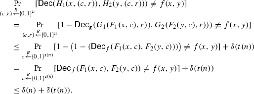
Assume that for all n, each function \(f : {\{0,1\}}^n \times {\{0,1\}}^n \rightarrow {\{0,1\}}\) has a \(\delta (n)\)-correct \(\varepsilon (n)\)-private \(\mathsf {1PSM}\) protocol with communication complexity t(n) and randomness complexity s(n). Then, each f has a \([\delta (n) + \delta (t(n))]\)-correct \(\max (\varepsilon (n),\delta (n)+\varepsilon (t(n)))\)-private \(\mathsf {PSM}\) protocol with communication complexity t(t(n)) and randomness complexity \(s(n) + s(t(n))\). In particular, if every such f has a \(\mathsf {1PSM}\) with \(\hbox {poly}(n)\) communication and randomness, and negligible privacy and correctness errors of \(n^{-\omega (1)}\), then every f has a \(\mathsf {PSM}\) with \(\hbox {poly}(n)\) communication and randomness, and negligible privacy and correctness errors of \(n^{-\omega (1)}\).
An important open question in information-theoretic cryptography is whether every function \(f : {\{0,1\}}^n \times {\{0,1\}}^n \rightarrow {\{0,1\}}\) admits a \(\mathsf {PSM}\) whose communication and randomness complexity are polynomial in n and its privacy and correctness errors are negligible in n. Therefore, by Theorem 2.4, constructing \(\mathsf {1PSM}\) with such parameters would be considered to be a major breakthrough. Together with Theorem 2.3, we conclude that it will be highly non-trivial to discover randomness-efficient \(\mathsf {ZAM}\) protocols for general functions.
2.4 Constructing \(\mathsf {CDS}\)
In the \(\mathsf {CDS}\) model [11], Alice holds an input x and Bob holds an input y, and, in addition, both parties hold a common secret bit b. The referee, Carol, holds both x and y, but it does not know the secret b. Similarly to the \(\mathsf {PSM}\) case, Alice and Bob use shared randomness to compute the messages \(m_1\) and \(m_2\) that are sent to Carol. The \(\mathsf {CDS}\) requires that Carol can recover b from \((m_1,m_2)\) iff \(f(x,y) = 1\). Moving to the complement \(\overline{f}=1-f\) of f, one can view the \(\mathsf {CDS}\) model as a variant of \(\mathsf {1PSM}\), in which the privacy leakage in case of 0-inputs is full, i.e., given the messages sent by Alice and Bob, one can recover their secret b but on 1-input b remains secret. (Note that x and y are assumed to be public in both cases.) Indeed, it is not hard to prove the following observation.
Theorem 2.5
Assume that the function f has a \(\delta \)-complete \(\varepsilon \)-private \(\mathsf {1PSM}\) with communication complexity t and randomness complexity s. Then the function \(\overline{f}=1-f\) has a \(\delta \)-correct and \(\varepsilon \)-private \(\mathsf {CDS}\) scheme with communication complexity t and randomness complexity s.
Clearly, one can combine the above theorem with the \(\mathsf {ZAM}\) to \(\mathsf {1PSM}\) transformation and get a transformation from \(\mathsf {ZAM}\) to \(\mathsf {CDS}\). However, one can do better by using a direct construction that avoids the overhead in the \(\mathsf {ZAM}\) to \(\mathsf {1PSM}\) transformation of Theorem 2.3.
Theorem 2.6
Assume that the function \(f : {\{0,1\}}^n \times {\{0,1\}}^n \rightarrow {\{0,1\}}\) has a \(\delta \)-sound \(\mathsf {ZAM}\) protocol with communication complexity \(\ell \) and randomness complexity m. Then the following hold.
-
1.
The function \(\overline{f}=1-f\) has a \(\delta \)-correct and 0-private \(\mathsf {CDS}\) with communication complexity m and randomness complexity 2m.
-
2.
For any \(t \in {\mathbb {N}}\), the function \(\overline{f}\) has a \((\delta + 2^{-t})\)-correct and \((2^{-t})\)-private \(\mathsf {CDS}\) with communication complexity m and randomness complexity \((\ell + t)\).
The communication complexity of \(\mathsf {CDS}\) protocols was studied in several previous works. Recently, it was shown by Ishai and Wee [18] that the \(\mathsf {CDS}\) complexity of f is linear in the size of the arithmetic branching program (ABP). (This improves the previous quadratic upper-bound of [11].) We can reprove this result by combining Theorem 2.6 with the \(\mathsf {ZAM}\) construction of [13] whose complexity is also linear in the ABP size of f. Interestingly, the resulting \(\mathsf {CDS}\) protocol is different from the construction of Ishai and Wee [18], and can be extended to work with dependency programs (DP). The latter model was introduced in [22] and can be viewed as a generalization of arithmetic branching program. (See Sect. 8 for a formal definition.) By applying the ideas of [13], we derive the following result.
Theorem 2.7
Assume that the function f has a dependency program of size m. Then, for every \(t\in {\mathbb {N}}\), the function f has an \(2^{-t}\)-correct perfectly private \(\mathsf {CDS}\) scheme with randomness complexity and communication complexity of \(O(m \cdot t)\).
The theorem extends to the case where the secret is a field element (see Theorem 8.2) and to the case where f is computed by an arithmetic dependency program and so its inputs are also field elements (see Remark 8.4). To the best of our knowledge, Theorem 2.7 yields the first CDS whose complexity is linear in the dependency program of the underlying function. This is incomparable to the best previous result, implicit in [18, Section 7], which achieves linear dependency in the size of the arithmetic span program (ASP) [21] that computes f.Footnote 3 Indeed, it is known that the size of the smallest dependency program of a function is polynomially related to the size of its smallest span program, but the transformation from one model to the other may incur some polynomial overhead [6]. Hence, for some functions, Theorem 2.7 can potentially lead to polynomial improvement over the ASP- (and ABP-) based schemes. On the other hand, the construction of [18] achieves perfect correctness, while our construction suffers from a nonzero decoding error.Footnote 4 We further mention that our construction can be viewed as dual to the construction of [18]; See Remark 8.5. Finally, we note that \(\mathsf {CDS}\) protocols have recently found applications in attribute-based encryption (see [12]). For this application, the \(\mathsf {CDS}\) is required to satisfy some linearity properties which hold for our \(\mathsf {CDS}\)-based construction. (See Remark 8.3.)
3 Preliminaries
For an integer \(n \in {\mathbb {N}}\), let \([n]=\{1,\ldots ,n\}\). The complement of a bit b is denoted by \(\overline{b} = 1 - b\). For a set S, we let \(S^k\) be the set of all possible k-tuples with entries in S, and for a distribution D, we let \(D^k\) be the probability distribution over k-tuples such that each tuple’s element is drawn according to D. We let \(s \mathop {\leftarrow }\limits ^{R}S\) denote an element that is sampled uniformly at random from the finite set S. The uniform distribution over n-bit strings is denoted by \(U_n\). For a boolean function \(f: S \rightarrow \{0,1\}\), we say that \(x \in S\) is 0-input if \(f(x)=0\), and is 1-input if \(f(x)=1\). A subset R of a product set \(A \times B\) is a rectangle if \(R=A' \times B'\) for some \(A'\subseteq X\) and \(B'\subseteq Y\).
The statistical distance between two random variables, X and Y, denoted by \(\Delta (X ; Y)\) is defined by \(\Delta (X ; Y):= \frac{1}{2}\sum _z \left| {\Pr [X = z] - \Pr [Y=z]}\right| \). We will also use statistical distance for probability distributions, where for a probability distribution D the value \(\Pr [D = z]\) is defined to be D(z).
We write \(\mathop {\Delta }\nolimits _{x_1 \mathop {\leftarrow }\limits ^{R}D_1, \ldots , x_k \mathop {\leftarrow }\limits ^{R}D_k}(F(x_1,\ldots ,x_k) ; G(x_1,\ldots ,x_k))\) to denote the statistical distance between two distributions obtained as a result of sampling \(x_i\)’s from \(D_i\)’s and applying the functions F and G to \((x_1,\ldots ,x_k)\), respectively. We use the following facts about the statistical distance. For every distributions X and Y and a function F (possibly randomized), we have that \(\Delta (F(X),F(Y)) \le \Delta (X,Y)\). In particular, for a boolean function F this implies that \(\Pr [F(X) = 1] \le \Pr [F(Y) = 1] + \Delta (X ; Y)\).
For a sequence of probability distributions \((D_1,\ldots ,D_k)\) and a probability vector \(W=(w_1,\ldots ,w_k)\), we let \(Z=\sum w_i D_i\) denote the “mixture distribution” obtained by sampling an index \(i\in [k]\) according to W and then outputting an element \(z \mathop {\leftarrow }\limits ^{R}D_i\).
Lemma 3.1
For any distribution \(Z=\sum w_i D_i\) and probability distribution S, it holds that
Proof
By the definition of statistical distance we can write \(\Delta (S ; Z)\) as
\(\square \)
4 Definitions
4.1 \(\mathsf {PSM}\)-Based Models
Definition 4.1
(\(\mathsf {PSM}\)) Let \(f: {\{0,1\}}^n \times {\{0,1\}}^n \rightarrow {\{0,1\}}\) be a boolean function. We say that a pair of (possibly randomizedFootnote 5) encoding algorithms \(F_1,F_2: {\{0,1\}}^n \times {\{0,1\}}^s \rightarrow {\{0,1\}}^t\) are \(\mathsf {PSM}\) for f if the function \(F(x,y,c)=(F_1(x,c),F_2(y,c))\) that corresponds to the joint computation of \(F_1\) and \(F_2\) on a common c, satisfy the following properties:
-
\(\delta \)-Correctness: There exists a deterministic algorithm \(\mathsf {Dec} \), called decoder, such that for every input (x, y) we have that
 (1)
(1) -
\(\varepsilon \)-Privacy: There exists a randomized algorithm (simulator) \(\mathsf {Sim} \) such that for any input (x, y) it holds that
$$\begin{aligned} \mathop {\Delta }\limits _{c \mathop {\leftarrow }\limits ^{R}{\{0,1\}}^s}(\mathsf {Sim} (f(x,y)) ; F(x,y,c)) \le \varepsilon . \end{aligned}$$(2)

The communication complexity of the \(\mathsf {PSM}\) protocol is defined as the encoding length t, and the randomness complexity of the protocol is defined as the length s of the common randomness.
One can also consider relaxations of this definition that are private only on a subset of inputs. We study such a relaxation \(\mathsf {1PSM}\) [1, 3] that is required to be private only on 1-inputs:
-
\(\varepsilon \)-Privacy on 1-inputs: There exists a simulator \(\mathsf {Sim} \) such that for any 1-input (x, y) of f it holds that
$$\begin{aligned} \mathop {\Delta }\limits _{c \mathop {\leftarrow }\limits ^{R}{\{0,1\}}^s}(\mathsf {Sim}, (F_1(x,c),F_2(y,c))) \le \varepsilon . \end{aligned}$$(3)
A stronger variant of \(\mathsf {PSM}\) is captured by the notion of perfect \(\mathsf {PSM}\) [1].
Definition 4.2
(\(\mathsf {pPSM}\)) Let \(f: {\{0,1\}}^n \times {\{0,1\}}^n \rightarrow {\{0,1\}}\). A pair of deterministic algorithms \(F_1,F_2: {\{0,1\}}^n \times {\{0,1\}}^s \rightarrow {\{0,1\}}^t\) is a \(\mathsf {pPSM}\) of f if \((F_1,F_2)\) is a 0-correct, 0-private \(\mathsf {PSM}\) of f such that:
-
Balance: There exists a 0-private (perfectly private) simulator \(\mathsf {Sim} \) such that \(\mathsf {Sim} (U_1) \equiv U_{2t}\).
-
Stretch-Preservation: We have that \(1 + s = 2t\).
Remark 4.3
(\(\mathsf {pPSM}\) – combinatorial view) One can also formulate the \(\mathsf {pPSM}\) definition combinatorially [1]: For f’s b-input (x, y), let \(F_{xy}(c)\) denote the joint output of the encoding \((F_1(x,c),F_2(y,c))\). Let \(S_b := \{F_{xy}(c)\ |\ c \in {\{0,1\}}^s, (x,y) \in f^{-1}(b)\}\) and let \(R={\{0,1\}}^t \times {\{0,1\}}^t\) denote the joint range of \((F_1,F_2)\). Then, \((F_1,F_2)\) is a \(\mathsf {pPSM}\) of f if and only if (1) The 0-image \(S_0\) and the 1-image \(S_1\) are disjoint; (2) The union of \(S_0\) and \(S_1\) equals to the range R; and (3) for all (x, y) the function \(F_{xy}\) is a bijection on \(S_{f(x,y)}\). One can also consider a case when \(F_1\) and \(F_2\) have arbitrary ranges, i.e., \(F_i : {\{0,1\}}^n \times {\{0,1\}}^s \rightarrow {\{0,1\}}^{t_i}\). In this case we say that \((F_1,F_2)\) is a \(\mathsf {pPSM}\) of f if the above conditions hold with respect to the joint range \(R={\{0,1\}}^{t_1}\times {\{0,1\}}^{t_2}\).
We consider a variant of \(\mathsf {CDS}\) called conditional disclosure of the common secret [11]. As in \(\mathsf {PSM}\), Alice and Bob hold the inputs x and y, respectively, and, in addition, both parties get a secret \(b\in {\{0,1\}}\). The goal is to reveal the secret to an external referee Carol only if some predicate f(x, y) evaluates to 1. Unlike the \(\mathsf {PSM}\) model, we assume that Carol knows both x and y. Formally, a \(\mathsf {CDS}\) scheme is defined below.
Definition 4.4
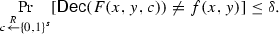
(\(\mathsf {CDS}\)) Let \(f: {\{0,1\}}^n \times {\{0,1\}}^n \rightarrow {\{0,1\}}\) be a predicate. Let \(F_1,F_2 : {\{0,1\}}^n \times {\{0,1\}}\times {\{0,1\}}^s \rightarrow {\{0,1\}}^t\) be (possibly randomized) encoding algorithms. Then, the pair \((F_1,F_2)\) is a \(\mathsf {CDS}\) scheme for f if and only if the function \(F(x,y,b,c)=(F_1(x,b,c),F_2(y,b,c))\) that corresponds to the joint computation of \(F_1\) and \(F_2\) on a common b and c, satisfies the following properties:
-
\(\delta \)-Correctness: There exists a deterministic algorithm \(\mathsf {Dec} \), called a decoder, such that for every 1-input (x, y) of f and any secret \(b \in {\{0,1\}}\) we have that
-
\(\varepsilon \)-Privacy: There exists a simulator \(\mathsf {Sim} \) such that for every 0-input (x, y) of f and any secret \(b \in {\{0,1\}}\) it holds that
$$\begin{aligned} \mathop {\Delta }\limits _{c \mathop {\leftarrow }\limits ^{R}{\{0,1\}}^s}(\mathsf {Sim} (x,y)\ ;\ F(x,y,b,c)) \le \varepsilon . \end{aligned}$$

Similarly to \(\mathsf {PSM}\), the communication complexity of the \(\mathsf {CDS}\) protocol is t and its randomness complexity is s.
The above definition naturally extends to the case where the secret comes from some non-binary domain B, and where the domain of the randomness and of the output of \(F_1\) and \(F_2\) is taken to be some arbitrary finite set. (When the output domain \(Z_1\) of \(F_1\) and \(Z_2\) of \(F_2\) differ, we define the communication complexity to be \(\max _i \log |Z_i|\).)
Remark 4.5
(CDS and PSM as Randomized Encoding) We can view \(\mathsf {PSM}\) and \(\mathsf {CDS}\) protocols under the framework of randomized encodings of functions (RE) [1, 15]. Formally, a function F(x, y, c) is a \(\delta \)-correct \(\varepsilon \)-private RE of f(x, y) if F(x, y) satisfies Eqs. (1) and (2) from Definition 4.1. Under this terminology, \(\mathsf {PSM}\) is simply an encoding F(x, y, c) which can be decomposed into two parts, \(F_1\) which depends on x and c but not on y and \(F_2\) which depends on y and c but not on x. Similarly, the notion of \(\mathsf {pPSM}\) and \(\mathsf {1PSM}\) can be derived by considering 2-decomposable perfect encodings and 2-decomposable encoding with 1-sided privacy. We further mention that a \(\mathsf {CDS} \) can be also viewed as a randomized encoding. Indeed, \((F_1,F_2)\) is a \(\mathsf {CDS} \) of f if and only if \(F(x,y,b,c)=(x,y,F_1(x,b,c),F_2(y,b,c))\) encodes the (non-boolean) function \(g(x,y,b)=(x,y,f(x,y)\wedge b)\).
4.2 ZAM
Definition 4.6
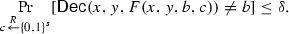
(\(\mathsf {ZAM}\)) Let \(f: {\{0,1\}}^n \times {\{0,1\}}^n \rightarrow {\{0,1\}}\). We say that a pair of deterministic boolean functions \(A,B: {\{0,1\}}^n \times {\{0,1\}}^m \times {\{0,1\}}^\ell \rightarrow {\{0,1\}}\) is a \(\mathsf {ZAM}\) for f if the predicate \({\mathsf {Accept}}(x,y,r_A,r_B,p)=A(x,r_A,p)\wedge B(y,r_B,p)\) satisfies the following properties:
-
Unambiguous Completeness: For any 1-input (x, y) and any randomness \((r_A,r_B) \in {\{0,1\}}^m \times {\{0,1\}}^m\) there exists a unique \(p \in {\{0,1\}}^\ell \) such that \({\mathsf {Accept}}(x,y,r_A,r_B,p)=1\).
-
Zero-Information: There exists a distribution D on the proof space \({\{0,1\}}^\ell \) such that for any 1-input (x, y) we have that

The distribution D is called the accepting distribution.
-
\(\delta \)-Soundness: For any 0-input (x, y) it holds that


The communication complexity (resp., randomness complexity) of the \(\mathsf {ZAM}\) protocol is defined as the length \(\ell \) of the proof (resp., the length m of the local randomness).
The Zero-Information property asserts that for every accepting input (x, y) the distribution \(D_{x,y}\), obtained by sampling \(r_A\) and \(r_B\) and outputting the (unique) proof p which is accepted by Alice and Bob, is identical to a single universal distribution D.
Following [13], we sometimes refer to the proofs as “rectangles” because for each (x, y) a proof p naturally corresponds to a set of points
which forms a rectangle in \({\{0,1\}}^m \times {\{0,1\}}^m\).
5 From \(\mathsf {pPSM}\) to \(\mathsf {ZAM}\)
In this section we construct a \(\mathsf {ZAM}\) scheme from a \(\mathsf {pPSM}\) protocol. By exploiting the combinatorial structure of \(\mathsf {pPSM}\), for each input (x, y) we construct a function \(h_{xy}\) that is a bijection if (x, y) is a 1-input and is two-to-one if (x, y) is a 0-input. In the constructed \(\mathsf {ZAM}\) scheme Alice and Bob use their local randomness to sample a uniform point in h’s range (Alice samples its x-coordinate \(r_A\) and Bob samples its y-coordinate \(r_B\)). Merlin’s proof is the preimage p for the sampled point, i.e., a point p such that \(h_{xy}(p) = (r_A,r_B)\). In order to accept the proof p, Alice and Bob verify that it is a preimage for the sampled point \((r_A,r_B)\).
First, the constructed \(\mathsf {ZAM}\) is unambiguously complete because \(h_{xy}\) is a bijection if (x, y) is a 1-input of f. Second, the constructed \(\mathsf {ZAM}\) satisfies the Zero-Information property because the distribution of the accepted proofs is uniform. Third, the constructed \(\mathsf {ZAM}\) is sound, because if (x, y) is a 0-input, then \(h_{xy}\) is two-to-one, implying that with probability at least 1 / 2 no preimage exists.
Theorem 2.1. Let f be a function with a \(\mathsf {pPSM}\) protocol that has communication complexity t and randomness complexity s. Then f has a 1 / 2-sound \(\mathsf {ZAM}\) scheme with randomness complexity of t and communication complexity of \(s+1\).
Proof
Let \(f:{\{0,1\}}^n \times {\{0,1\}}^n \rightarrow {\{0,1\}}\) be a function with a \(\mathsf {pPSM}\) \(F_1,F_2:{\{0,1\}}^n \times {\{0,1\}}^s \rightarrow {\{0,1\}}^t\). We show that there exists a 1 / 2-sound \(\mathsf {ZAM} \) protocol for f with Alice’s and Bob’s local randomness spaces \({\{0,1\}}^m\) and proof space \({\{0,1\}}^\ell \) where \(m = t\) and \(\ell = 2t\).
First, we prove some auxiliary statement about \(\mathsf {pPSM}\). Let \(g(x,y,c) := (F_1(x,c),F_2(y,c))\). For any (x, y), we define a new function \(h_{xy}: {\{0,1\}}^s \times {\{0,1\}}\rightarrow {\{0,1\}}^t \times {\{0,1\}}^t\) as follows.
The function h satisfies the following useful properties as follows from the combinatorial view of \(\mathsf {pPSM}\) (Remark 4.3).
Fact 5.1
If (x, y) is a 1-input for f, then the function \(h_{xy}\) is a bijection. Otherwise, if (x, y) is a 0-input for f, then the image of the function \(h_{xy}\) covers exactly half of the range \({\{0,1\}}^t \times {\{0,1\}}^t\).
We now describe a \(\mathsf {ZAM}\) protocol for f in which the local randomness of Alice and Bob is sampled from \({\{0,1\}}^t\), and the proof space is \({\{0,1\}}^s \times {\{0,1\}}\). Recall that \((F_1,F_2)\) is a \(\mathsf {pPSM}\) and therefore \(s+1=2t\) and \({\{0,1\}}^s \times {\{0,1\}}={\{0,1\}}^{2t}\). The \(\mathsf {ZAM}\) ’s accepting functions A, B are defined as follows:
Observe that the following equivalence holds.
Claim 5.2
\(\forall x,y,c,b,m_1,m_2\ \Big [h_{xy}(c,b) = (m_1,m_2)\Big ] \Leftrightarrow \big [A(x,m_1,(c,b)) = 1 = B(y,m_2,(c,b))\big ]\).
Now we verify that (A, B) is \(\mathsf {ZAM} \) for f:
-
Unambiguous Completeness: Consider any f’s 1-input (x, y) and take any \((m_1,m_2) \in {\{0,1\}}^t \times {\{0,1\}}^t\). Since (x, y) is a 1-input for f, we have that \(h_{xy}\) is a bijection. This means that there exists a unique (c, b) such that \(h_{xy}(c,b)=(m_1,m_2)\). By Claim 5.2, this proof (c, b) is the only proof which is accepted by both Alice and Bob when the randomness is set to \(m_1,m_2\).
-
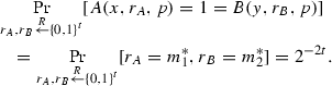
Zero-Information: We show that the accepting distribution is uniform, i.e., for any 1-input (x, y) and for any \(p \in {\{0,1\}}^s \times {\{0,1\}}\) it holds that
Take any 1-input (x, y). Since (x, y) is a 1-input for f, we have that \(h_{xy}\) is a bijection. Hence, there exists a unique \((m_1^*,m_2^*) \in {\{0,1\}}^n \times {\{0,1\}}^n\) such that \(h_{xy}(c,b)=(m_1^*,m_2^*)\). By Claim 5.2, this means that Alice and Bob accept only this \((m_1^*,m_2^*)\). Hence, for all proofs p we have that
-
1 / 2-Soundness: Fix some 0-input (x, y), and recall that the image H of \(h_{xy}\) covers exactly half of the range \({\{0,1\}}^t \times {\{0,1\}}^t\), i.e., \(|H| = \left| {{\{0,1\}}^t \times {\{0,1\}}^t}\right| /2\). It follows that, with probability 1 / 2, the randomness of Alice and Bob \((m_1,m_2)\) chosen randomly from \({\{0,1\}}^t \times {\{0,1\}}^t\) lands outside H. In this case, the set \(h^{-1}_{xy}(m_1,m_2)\) is empty and so there is no proof (c, b) that will be accepted.\(\square \)


6 From \(\mathsf {ZAM}\) to \(\mathsf {1PSM}\)
In this section we construct \(\mathsf {1PSM}\) protocols from a \(\mathsf {ZAM}\) scheme and prove Theorem 2.3 (restated here for convenience).
Theorem 2.3. Let \(f : {\{0,1\}}^n \times {\{0,1\}}^n \rightarrow {\{0,1\}}\) be a function with a \(\delta \)-sound \(\mathsf {ZAM}\) protocol that has communication complexity \(\ell \) and randomness complexity m. Then, for all \(k \in {\mathbb {N}}\), the following hold:
-
1.
f has \((2^{2n} \delta ^k)\)-correct and 0-private \(\mathsf {1PSM}\) with communication complexity of km and 2k m bits of shared randomness.
-
2.
f has \((2^{2n} \delta ^k + 2^{-\ell k})\)-correct and \((2^{-\ell k})\)-private \(\mathsf {1PSM}\) with communication complexity of km and \(2 \ell k\) bits of shared randomness.
Proof
Let \(f: {\{0,1\}}^n \times {\{0,1\}}^n \rightarrow {\{0,1\}}\) be a function with a \(\delta \)-sound \(\mathsf {ZAM}\) protocol (A, B) with Alice’s and Bob’s local randomness spaces \({\{0,1\}}^m\) and the proof space \({\{0,1\}}^\ell \). Fix some integer k. We start by constructing the first \(\mathsf {1PSM}\) protocol.
We first define some additional notation and prove auxiliary claims. For a pair of inputs (x, y) let
and \(Z := \bigcup _{(x,y) \in f^{-1}(0)} E_{xy}^k\).
Claim 6.1
\(|Z| \le 2^{2n} (\delta 2^{2m})^k\).
Proof
By the soundness property of \(\mathsf {ZAM}\), we have that \(|E_{xy}| \le \delta 2^{2m}\) for any 0-input (x, y). Hence, each \(|E_{xy}^k| \le (\delta 2^{2m})^k\). We conclude that
\(\square \)
Let \({\mathcal {A}} ^x_p := \{ r_A \in {\{0,1\}}^m\ |\ {A(x,r_A,p) = 1}\}\) and \({\mathcal {B}} ^y_p := \{ r_B \in {\{0,1\}}^m\ |\ {B(y,r_B,p) = 1}\}\).
Claim 6.2
Let \(D_{\textsc {acc}}\) be the accepting distribution of \(\mathsf {ZAM}\). Then, for any 1-input (x, y) and \(p \in {\{0,1\}}^\ell \) we have that \(D_{\textsc {acc}}(p) = 2^{-2m} |{\mathcal {A}} ^x_p||{\mathcal {B}} ^y_p|\).
Proof
By definition
In order to derive the claim, note that since every proof forms a “rectangle” (see Sect. 4.2), we have that
\(\square \)
We can now describe the encoding algorithms \(G_1\) and \(G_2\) and the decoder \(\mathsf {Dec} \). First, \(G_1\) and \(G_2\) use the shared randomness to sample a proof p according to the accepting distribution. Then \(G_1\) and \(G_2\) sample (private) randomness that can lead to the acceptance of p on their input (x, y), i.e., \(G_1\) computes \(a \mathop {\leftarrow }\limits ^{R}{\mathcal {A}} _p^x\) and \(G_2\) computes \(b \mathop {\leftarrow }\limits ^{R}{\mathcal {B}} _p^y\). We have that if \(f(x,y) = 1\) then (a, b) is distributed uniformly, while if \(f(x,y) = 0\) then (a, b) is sampled from the set Z. The task of the decoder is to verify whether it is likely that a point has been sampled from Z or uniformly. This is achieved by repeating the protocol k times. Below is the formal description of the algorithms \(G_1,G_2\), and decoder.

Let us verify that the proposed protocol is a \(\mathsf {1PSM}\) for f.
\((2^{2n} \delta ^k)\)-Correctness. Since that the decoder never errs on 0-inputs, it suffices to analyze the probability that some 1-input (x, y) is incorrectly decoded to 0. Fix some 1-input (x, y). Below we will show that the message \(\mathbf {s} = ((a_1,b_1),\ldots ,(a_k,b_k))\) generated by the encoders \(G_1\) and \(G_2\) is uniformly distributed over the set \(({\{0,1\}}^m \times {\{0,1\}}^m)^k\). Hence, the probability that \(\mathbf {s}\) lands in Z (and decoded incorrectly to 0) is exactly \(\frac{|Z|}{|({\{0,1\}}^m \times {\{0,1\}}^m)^k|}\), which, by Claim 6.1, is upper-bounded by \(2^{2n}\delta ^k\).
It is left to show that \(\mathbf {s}\) is uniformly distributed. To see this, consider the marginalization of \((a_i,b_i)\)’s probability distribution: For a fixed \((r_A,r_B)\) we have that
Because of the unambiguous completeness property of \(\mathsf {ZAM}\), we have that there exists a single \(p^{*}\) such that \((r_A,r_B) \in {\mathcal {A}} ^x_{p^*} \times {\mathcal {B}} ^y_{p^*}\). Hence, all probabilities \(\Pr [(a_i,b_i) = (r_A,r_B)\ |\ p_i = p]\) are zero, if \(p \ne p^{*}\). This implies that
We have that \(\Pr [p_i = p] = D_{\textsc {acc}}(p) = 2^{-2m}{|{\mathcal {A}} ^x_p||{\mathcal {B}} ^y_p|}\) (due to Claim 6.2), and \(\Pr [(a_i,b_i) = (r_A,r_B)\ |\ p_i = p^{*}]\) is \(\frac{1}{|{\mathcal {A}} ^x_p|\cdot |{\mathcal {B}} ^y_p|}\) by the construction of the encoding functions. Hence, \(\Pr [(a_i,b_i)=(r_A,r_B)] = 2^{-2m}\). Because all pairs \((a_i,b_i)\) are sampled independently, we get that the combined tuple \(\mathbf {s} = ((a_1,b_1),\ldots ,(a_k,b_k))\) is sampled uniformly from \(({\{0,1\}}^m \times {\{0,1\}}^m)^k\), as required.
Privacy for 1-inputs. As shown above, if (x, y) is a 1-input, then \(\mathbf {s}\) is uniformly distributed over \(({\{0,1\}}^m \times {\{0,1\}}^m)^k\). Hence, the simulator for proving the privacy property of \(\mathsf {PSM}\) can be defined as a uniform sampler from \(({\{0,1\}}^m \times {\{0,1\}}^m)^k\).
The second protocol. The second item of the theorem is proved by using the first protocol, except that the point \(\mathbf {p}=(p_1,\ldots , p_k)\) is sampled from a different distribution \(D'\). For a parameter t, the distribution \(D'\) is simply the distribution \(D_{\textsc {acc}}^k\) discretized into \(2^{-(\ell k + t)}\)-size intervals. Such \(D'\) can be sampled using only \(\ell k + t\) random bits. Moreover, for each point \(\mathbf {p}\), the difference between \(D_{\textsc {acc}}^k(\mathbf {p})\) and \(D'(\mathbf {p})\) is at most \(2^{-(\ell k + t)}\). Since the support of \(D_{\textsc {acc}}^k\) is of size at most \(2^{\ell k}\), it follows that \(\Delta (D';D_{\textsc {acc}}^k)\le 2^{-(\ell k + t)} \cdot 2^{\ell k} = 2^{-t}\). As a result, we introduce an additional error of \(2^{-t}\) in both privacy and correctness. By setting t to \(\ell k\), we derive the second \(\mathsf {1PSM}\) protocol.\(\square \)
7 From \(\mathsf {1PSM}\) to \(\mathsf {PSM}\)
In this section we show how to upgrade a \(\mathsf {1PSM}\) protocol into a \(\mathsf {PSM}\) protocol. We assume that we have a way of constructing \(\mathsf {1PSM}\) for all functions. Our main idea is to reduce a construction of a \(\mathsf {PSM}\) scheme for f to two \(\mathsf {1PSM}\) schemes. The first \(\mathsf {1PSM}\) scheme computes the function f, and the second \(\mathsf {1PSM}\) scheme computes the function \(\overline{\mathsf {Dec} _f}\), i.e., the complement of the decoder \(\mathsf {Dec} _f\) of the first scheme. We show how to combine the two schemes such that the first scheme protects the privacy of 1-inputs and the second scheme protects the privacy of 0-inputs.
Theorem 2.4. Assume that for all n, each function \(f : {\{0,1\}}^n \times {\{0,1\}}^n \rightarrow {\{0,1\}}\) has a \(\delta (n)\)-correct \(\varepsilon (n)\)-private \(\mathsf {1PSM}\) protocol with communication complexity t(n) and randomness complexity s(n). Then, each f has a \([\delta (n) + \delta (t(n))]\)-correct \(\max (\varepsilon (n),\delta (n)+\varepsilon (t(n)))\)-private \(\mathsf {PSM}\) protocol with communication complexity t(t(n)) and randomness complexity \(s(n) + s(t(n))\). In particular, if every such f has a \(\mathsf {1PSM}\) with \(\hbox {poly}(n)\) communication and randomness, and negligible privacy and correctness errors of \(n^{-\omega (1)}\), then every f has a \(\mathsf {PSM}\) with \(\hbox {poly}(n)\) communication and randomness, and negligible privacy and correctness errors of \(n^{-\omega (1)}\).
Proof
Let \(f : {\{0,1\}}^n \times {\{0,1\}}^n \rightarrow \{0,1\}\). Let \(F_1,F_2: {\{0,1\}}^n \times {\{0,1\}}^{s(n)} \rightarrow {\{0,1\}}^{t(n)}\) be a \(\delta (n)\)-correct and \(\varepsilon (n)\)-private on 1 inputs \(\mathsf {1PSM}\) for f with decoder \(\mathsf {Dec} _f\) and simulator \(\mathsf {Sim} _f\). Define a function \(g: {\{0,1\}}^{t(n)} \times {\{0,1\}}^{t(n)} \rightarrow \{0,1\}\) to be \(1-\mathsf {Dec} _f(m_1,m_2)\). Let \(G_1,G_2: {\{0,1\}}^{t(n)} \times {\{0,1\}}^{s(t(n))} \rightarrow {\{0,1\}}^{t(t(n))}\) be a \(\delta (t(n))\)-correct and \(\varepsilon (t(n))\)-private on 1 inputs \(\mathsf {1PSM}\) for g with decoder \(\mathsf {Dec} _g\) and simulator \(\mathsf {Sim} _g\).
We construct a (standard) \(\mathsf {PSM}\) for f as follows. Let \({\{0,1\}}^u = {\{0,1\}}^{s(n)} \times {\{0,1\}}^{s(t(n))}\) be the space of shared randomness, let \({\{0,1\}}^v = {\{0,1\}}^{t(t(n))}\) be the output space and define the encoding functions \(H_1,H_2: {\{0,1\}}^n \times {\{0,1\}}^u \rightarrow {\{0,1\}}^v\), by
We show that \((H_1,H_2)\) is a \(\mathsf {PSM}\) by verifying its security properties.
-
\(\delta (n) + \delta (t(n))\)-Correctness: On an input \((e_1,e_2)\) define the decoding algorithm \(\mathsf {Dec} \) to output \(1-\mathsf {Dec} _g(e_1,e_2)\). The decoding algorithm \(\mathsf {Dec} \) works correctly whenever both \(\mathsf {Dec} _g\) and \(\mathsf {Dec} _f\) succeed. Hence, the error probability for decoding can be bounded as follows:
-
\(\varepsilon \)-Privacy: We define the simulator \(\mathsf {Sim} \) as follows: on 0-inputs it outputs \(\mathsf {Sim} _g\) and on 1-inputs it computes \(\mathsf {Sim} _f = (m_1,m_2)\), randomly samples r from \({\{0,1\}}^{s(t(n))}\), and outputs \((G_1(m_1,r),G_2(m_2,r))\). We verify that the simulator truthfully simulates the randomized encoding \((H_1,H_2)\) with deviation error of at most \(\varepsilon \).

We begin with the case where (x, y) is a 0-input for f. For any c, let \(L_c\) denote the distribution of the random variable \((G_1(F_1(x,c),r),G_2(F_2(y,c),r))\) where \(r \mathop {\leftarrow }\limits ^{R}{\{0,1\}}^{s(t(n))}\). Let M denote the “mixture distribution” which is defined by first sampling \(c \mathop {\leftarrow }\limits ^{R}{\{0,1\}}^{s(n)}\) and then outputting a random sample from \(L_c\), that is, the distribution \(M=\sum _{c \in {\{0,1\}}^{s(n)}} \Pr [U_{s(n)} = c] L_c\). Due to Lemma 3.1, we have that
Let C denote a subset of \(c \in {\{0,1\}}^{s(n)}\) such that \((F_1(x,c),F_2(y,c))\) is a 1-input for g. The set C satisfies the following two properties: (1) \(\forall c \in C \Delta (\mathsf {Sim} _g ; L_c) \le \varepsilon (t(n))\) and (2) \(|C|/2^{s(n)} \ge 1-\delta (n)\). The property (1) holds because \(G_1,G_2\) is private on 1-inputs of g. The property (2) holds because \(\mathsf {Dec} _f\) decodes correctly with the probability at least \(1 - \delta (n)\). After splitting the mixture sum in two, we have that
Because of the properties of C, we have that the first sum is upperbounded by \(\varepsilon (t(n))\) and the second one is upperbounded by \(\delta (n)\). This implies that \(\Delta (\mathsf {Sim} _g; M) {\le } \delta (n) + \varepsilon (t(n))\).
We move on to the case where (x, y) is a 1-input. Then
Consider the randomized procedure G which, given \((m_1,m_2)\), samples \(r\mathop {\leftarrow }\limits ^{R}{\{0,1\}}^{s(t(n))}\) and outputs the pair \((G_1(m_1,r),G_2(m_2,r))\). Applying G to the above distributions we get:
Recall that, for a random \(r\mathop {\leftarrow }\limits ^{R}{\{0,1\}}^{s(t(n)}\), it holds that \(G(\mathsf {Sim} _f;r) \equiv \mathsf {Sim} (1)\), and for every r, \(G(F_1(x,c),F_2(y,c);r)=(H_1(x,(c,r)),H_2(y,(c,r)))\). Hence, Eq. 4 can be written as
Since \(\varepsilon (n) \le \max (\varepsilon (n),\delta (n)+\varepsilon (t(n)))\), the theorem follows.\(\square \)
8 Constructing \(\mathsf {CDS}\) Schemes
8.1 From \(\mathsf {1PSM}\) to \(\mathsf {CDS}\)
In this section we construct a \(\mathsf {CDS}\) scheme from a \(\mathsf {1PSM}\) protocol. Our construction is based on the observation (due to [11]) that constructing a \(\mathsf {CDS}\) scheme for a function f can be reduced to constructing a \(\mathsf {PSM}\) scheme for the sharing function \(f'((x,s),(y,s)) = f(x,y) \wedge s\). We show that one can strengthen this statement by substituting \(\mathsf {PSM}\) with a weaker security primitive \(\mathsf {1PSM}\).
Theorem 2.5. Assume that the function f has a \(\delta \)-complete \(\varepsilon \)-private \(\mathsf {1PSM}\) with communication complexity t and randomness complexity s. Then the function \(\overline{f}=1-f\) has a \(\delta \)-correct and \(\varepsilon \)-private \(\mathsf {CDS}\) scheme with communication complexity t and randomness complexity s.
Proof
Let \(f : {\{0,1\}}^n \times {\{0,1\}}^n \rightarrow {\{0,1\}}\). Let \(F_1,F_2 : {\{0,1\}}^n \times {\{0,1\}}^s \rightarrow {\{0,1\}}^t\) be a \(\delta \)-correct and \(\varepsilon \)-private on 1-inputs \(\mathsf {1PSM}\) for f with decoder \(\mathsf {Dec} _f\) and simulator \(\mathsf {Sim} _f\). Let g denote \(1-f\). Then, \((F_1,F_2)\) is \(\delta \)-correct and \(\varepsilon \)-private on 0-inputs \(\mathsf {1PSM}\) for g with \(\mathsf {Dec} _g = 1-\mathsf {Dec} _f\) and \(\mathsf {Sim} _g = \mathsf {Sim} _f\).
We construct a \(\mathsf {CDS}\) scheme \((H_1, H_2)\) for g as follows. Let \((x_0,y_0)\) be some fixed 0-input of g. We define \(H_1(x,b,c)\) to output \(F_1(x_0,c)\) if \(b=0\), and \(F_1(x,c)\) if \(b=1\). Similarly, \(H_2(y,b,c)\) outputs \(F_2(y_0,c)\) if \(b=0\) and \(F_2(y,c)\) if \(b=1\). The decoder \(\mathsf {Dec} \) simply applies the \(\mathsf {1PSM}\) decoder of g, namely: given two messages \(m_1\) and \(m_2\), we reconstruct the secret b by outputting \(\mathsf {Dec} _g(m_1,m_2)\). We define the simulator \(\mathsf {Sim} \) to run the simulator \(\mathsf {Sim} _g\).
We prove that the pair \((H_1,H_2)\) is a \(\mathsf {CDS}\) scheme for g.
-
\(\delta \)-Correctness: Take any 1-input (x, y) of g:
-
If \(b=0\) then \(m_1 = F_1(x_0,c)\) and \(m_2 = F_2(y_0,c)\). By the correctness property of \(\mathsf {1PSM}\), we have that \(\mathsf {Dec} _g(m_1,m_2) = \mathsf {Dec} _g(F_1(x_0,c),F_2(y_0,c)) = g(x_0,y_0) = 0\) except with probability \(\delta \).
-
If \(b=1\) then \(m_1 = F_1(x,c)\) and \(m_2 = F_2(y,c)\). By the correctness property of \(\mathsf {1PSM}\), we have that \(\mathsf {Dec} _g(m_1,m_2) = \mathsf {Dec} _g(F_1(x,c),F_2(y,c)) = g(x,y) = 1\) except with probability \(\delta \).
-
\(\varepsilon \)-Privacy: Fix some 0-input (x, y) of g. Then, by the 1-sided privacy of the \(\mathsf {1PSM}\), we have that, for \(b=0\),
$$\begin{aligned}&\mathop {\Delta }\limits _{c \mathop {\leftarrow }\limits ^{R}{\{0,1\}}^s}(\mathsf {Sim} (x,y) ; (H_1(x, 0, c),H_2(y, 0, c))) \\&\quad = \mathop {\Delta }\limits _{c \mathop {\leftarrow }\limits ^{R}{\{0,1\}}^s} (\mathsf {Sim} _g ; (F_1(x_0,c),F_2(y_0,c)) ) \le \varepsilon , \end{aligned}$$and, for \(b=1\),
$$\begin{aligned}&\mathop {\Delta }\limits _{c \mathop {\leftarrow }\limits ^{R}{\{0,1\}}^s}(\mathsf {Sim} (x,y) ; (H_1(x, 1, c),H_2(y, 1, c))) \\&\quad = \mathop {\Delta }\limits _{c \mathop {\leftarrow }\limits ^{R}{\{0,1\}}^s} (\mathsf {Sim} _g ; (F_1(x,c),F_2(y,c)) ) \le \varepsilon . \end{aligned}$$
\(\square \)
8.2 From \(\mathsf {ZAM}\) to \(\mathsf {CDS}\)
We now describe a direct construction of \(\mathsf {CDS}\) from \(\mathsf {ZAM}\) that avoids the overhead in the transformation from \(\mathsf {ZAM}\) to \(\mathsf {1PSM}\) (Theorem 2.3). The saving is mainly due to the fact that, unlike the \(\mathsf {1PSM}\) setting, in the \(\mathsf {CDS}\) setting the decoder is allowed to depend on the inputs (x, y).
Theorem 2.6. Assume that the function \(f : {\{0,1\}}^n \times {\{0,1\}}^n \rightarrow {\{0,1\}}\) has a \(\delta \)-sound \(\mathsf {ZAM}\) protocol with communication complexity \(\ell \) and randomness complexity m. Then the following hold.
-
1.
The function \(\overline{f}=1-f\) has a \(\delta \)-correct and 0-private \(\mathsf {CDS}\) with communication complexity m and randomness complexity 2m.
-
2.
For any \(t \in {\mathbb {N}}\), the function \(\overline{f}\) has a \((\delta + 2^{-t})\)-correct and \((2^{-t})\)-private \(\mathsf {CDS}\) with communication complexity m and randomness complexity \((\ell + t)\).
Proof
Let \(f: {\{0,1\}}^n \times {\{0,1\}}^n \rightarrow {\{0,1\}}\) be a function with a \(\delta \)-sound \(\mathsf {ZAM}\) protocol (A, B) with randomness complexity of m and communication complexity of \(\ell \). Fix some integer k. We start by recalling some notation from Theorem 2.3. For a pair of inputs (x, y) let
Let \({\mathcal {A}} ^x_p := \{ r_A \in {\{0,1\}}^m\ |\ {A(x,r_A,p) = 1}\}\) and \({\mathcal {B}} ^y_p := \{ r_B \in {\{0,1\}}^m\ |\ {B(y,r_B,p) = 1}\}\).
We construct a \(\mathsf {CDS}\) scheme \((F_1, F_2)\) for g as follows. As common randomness the scheme takes p sampled from the accepting distribution \(D_{\textsc {acc}}\) of the \(\mathsf {ZAM}\) scheme (as in Theorem 2.3, \(D_{\textsc {acc}}\) can be perfectly simulated using 2m uniform bits). On an input (x, b, p) the function \(F_1\) computed by Alice outputs \(r_1 \mathop {\leftarrow }\limits ^{R}{\{0,1\}}^m\) if \(b=1\), and \(r_1 \mathop {\leftarrow }\limits ^{R}{\mathcal {A}} ^x_p\), otherwise. Similarly, on an input (y, b, p) the function \(F_2\) computed by Bob outputs \(r_2 \mathop {\leftarrow }\limits ^{R}{\{0,1\}}^m\) if \(b=1\), and \(r_2 \mathop {\leftarrow }\limits ^{R}{\mathcal {B}} ^y_p\), otherwise. The decoding procedure works as follows: on input \((x,y,r_1,r_2)\) the decoder outputs 0 if \((r_1,r_2) \in E_{xy}\), and 1 otherwise.
Now we prove that \((F_1,F_2)\) is a \(\mathsf {CDS}\) scheme for \(\overline{f}\) by verifying its security properties:
-
\(\delta \)-Correctness: Take any 1-input (x, y) of \(\overline{f}\), which is a 0-input of f.
-
If the secret bit \(b=0\), then \(r_1\) and \(r_2\) are sampled uniformly from \({\mathcal {A}} ^x_p\) and \({\mathcal {B}} ^y_p\), respectively. This means that with probability 1 the pair \((r_1,r_2)\) lands in \(E_{xy}\) and hence decoding of \((x,y,r_1,r_2)\) never fails in this case.
-
If the secret bit \(b=1\), then \(r_1\) and \(r_2\) are sampled uniformly from \({\{0,1\}}^m\). This implies that the probability that \((x,y,r_1,r_2)\) is decoded incorrectly to 0 is the probability of \((r_1,r_2)\) landing in \(E_{xy}\). Due to the soundness property of \(\mathsf {ZAM}\), the latter probability is at most \(\delta \).
-
Perfect Privacy: We define the simulator \(\mathsf {Sim} \) to output a random point \((r_1,r_2) \in {\{0,1\}}^m \times {\{0,1\}}^m\). Take any 0-input (x, y) of \(\overline{f}\), which is a 1-input of f. We verify that \(\mathsf {Sim} \) perfectly simulates the distribution of \((F_1,F_2)\) for any \(b \in {\{0,1\}}\). For \(b=0\) we have that \(F_1\) and \(F_2\) each output \(U_m\) by construction. For \(b=1\) we use the observation from the proof of Theorem 2.3 that the joint distribution of \((r_1,r_2)\) sampled from \({\mathcal {A}} ^x_p\) and \({\mathcal {B}} ^y_p\) for \(p \mathop {\leftarrow }\limits ^{R}D_{\textsc {acc}}\) is uniform over \({\{0,1\}}^m \times {\{0,1\}}^m\).
The second protocol. Similarly to Theorem 2.3, the second protocol is identical to the first protocol except it uses an approximation of \(D_{\textsc {acc}}\). We know that for any \(t \in {\mathbb {N}}\) the distribution \(D_{\textsc {acc}}\) can be approximated using \((\ell +t)\) bits at the cost of deviating by \(2^{-t}\) in terms of the statistical distance from \(D_{\textsc {acc}}\). This introduces an additional error of \(2^{-t}\) in both privacy and correctness of the second protocol.\(\square \)
8.3 \(\mathsf {CDS}\) for Dependency Programs
A dependency program is a model of computation introduced in [22]. The original model captures functions over binary inputs.
Definition 8.1
(\(\mathsf {DP}\)) A dependency program over a field \({\mathbb {F}}\) is a pair \((M,\rho )\), where M is a matrix over \({\mathbb {F}}\) and \(\rho \) is a labeling of the rows of M by the literals from \(\{x_1,\ldots ,x_n,\overline{x}_1,\ldots ,\overline{x}_n\}\) (every row is labeled with a single literal, and the same literal can be used in many rows). For an input \(u \in {\{0,1\}}^n\) let \(M_u\) denote the matrix obtained from M by selecting only the rows assigned to the literals satisfied by u, i.e., a row labeled with \(x_i\) (resp. \(\overline{x}_i\)) is chosen if the \(i^{{\textit{th}}}\) bit of u is 1 (resp., 0). A dependency program accepts an input u if and only if the rows of \(M_u\) are linearly dependent. A dependency program computes a Boolean function f if it accepts only 1-inputs of f. The size of the dependency program is the number of rows in M. We also write |M| to denote the number of row the matrix M has.
The number of columns s in \(\mathsf {DP}\) is not counted toward its size. Without loss of generality we may assume that s is upper-bounded by the number of rows (the size) since the matrix M can be restricted to a maximal set of linearly independent columns without changing the function that is computed (cf. [6, Remark 2.4]). It will also be convenient to assume that the number of rows labeled by \(x_i\) is equal to the number of rows that are labeled by its complement \(\bar{x}_i\). (If this is not the case and \(M_{x_i}\) contains less rows than \(M_{\bar{x}_i}\) then we can add new linearly independent rows labeled by \(x_i\), possibly at the expense of increasing the number of columns. Overall, the size of the resulting dependency program will be at most twice as large as the size of the original program.) Observe that if the input is partitioned between Alice and Bob, then the above convention guarantees that for every input x (resp., y) Alice (resp., Bob) will hold a matrix \(M_x\) (resp., \(M_y\)) with a fixed number of rows which is independent of the input.
We construct \(\mathsf {CDS}\) for dependency programs. The following theorem generalizes Theorem 2.7 from the introduction to arbitrary finite fields.
Theorem 8.2
(Theorem 2.7 generalized) Assume that the function \(f:{\{0,1\}}^n\times {\{0,1\}}^n\rightarrow {\{0,1\}}\) has a dependency program of size m over a finite field \({\mathbb {F}}\). Then, for every \(t\in {\mathbb {N}}\), the function f has an \((1/|{\mathbb {F}}|)^t\)-correct perfectly private \(\mathsf {CDS}\) scheme where the secret is an element of \({\mathbb {F}}\) and the protocol communicates \(O(m \cdot t)\) field elements and consumes \(O(m \cdot t)\) random field elements.
Note that for large fields, the scheme achieves low decoding error even for small values of t (e.g., 1).
Proof
Let \((M,\rho )\) be a dependency program for the function \(f: {\{0,1\}}^n \times {\{0,1\}}^n \rightarrow {\{0,1\}}\) over the finite field \({\mathbb {F}}\). Let s denote the number of columns in M, and let \(m_1\) (resp., \(m_2\)) denote the number of rows of M held by Alice for an input x (resp., held by Bob for an input y). Recall that, by convention, \(m_1\) and \(m_2\) are independent of x and y, and that \(m'=m_1+m_2\) is at most m, the size of M.
We present a basic \(\mathsf {CDS}\) scheme \((F_1, F_2)\) for f where the secret b can be an arbitrary field element. The scheme communicates at most 2m field elements, and uses at most 2m random field elements. It achieves perfect privacy and has a completeness error of \(1/|{\mathbb {F}}|\). In fact, the decoder will either output the right answer or will output, with probability \(1/|{\mathbb {F}}|\), a special failure symbol. Therefore, by repeating the protocol t times (with independent randomness), we can reduce the error to \(|{\mathbb {F}}|^{-t}\) with a multiplicative overhead of t in communication and randomness, as stated in the theorem.
The basic \(\mathsf {CDS}\) scheme \((F_1, F_2)\) is defined as follows. As common randomness the scheme takes a pair of random vectors \(c\in {\mathbb {F}}^s\) and \(d\in {\mathbb {F}}^{m'}\). On an input (x, b, c, d), the function \(F_1\) computed by Alice outputs the pair \((d_1,r_1)\) where \(d_1\in {\mathbb {F}}^{m_1}\) is the first \(m_1\) entries of the vector d, and \(r_1 = M_x \cdot c +b\cdot d_1\). (Recall that \(b\in {\mathbb {F}}\) is a scalar.) Similarly, on an input (y, b, c, d) the function \(F_2\) computed by Bob outputs the pair \((d_2,r_2)\) where \(d_2\in {\mathbb {F}}^{m_2}\) is the last \(m_2\) entries of the vector d and \(r_2 = M_y \cdot c+ b\cdot d_2\). For a 1-instance (x, y), the decoding procedure decodes \((d=(d_1,d_2), r=(r_1,r_2))\) as follows: (1) The decoder finds a nonzero vector \(v\in {\mathbb {F}}^{m'}\) for which \(v^{T}M_{xy}={\mathbf {0}}\) (such a vector must exist since the rows of \(M_{xy}\) are linearly dependent); (2) If the dot product \((v^T\cdot d)\) is nonzero the decoder outputs the value \(b'=(v^T\cdot r)/(v^T\cdot d)\), and otherwise it outputs a special failure symbol.
We prove that the pair \((F_1,F_2)\) is a \(\mathsf {CDS}\) for f.
-
Correctness: Fix some 1-input (x, y) of f. Since v is in the left nullspace of \(M_{xy}\), it holds that
$$\begin{aligned} v^T\cdot r= v^T (M_{xy} \cdot c + b\cdot d)= b\cdot (v^T\cdot d). \end{aligned}$$Therefore, decoding succeeds as long as \((v^T\cdot d)\ne 0\). The latter event happens with probability \(1-1/|{\mathbb {F}}|\) since \(d\in {\mathbb {F}}^{m'}\) is uniformly distributed.
-
Perfect Privacy: Fix some 0-input (x, y) of f. We show that in this case the random variables \((d_1,r_1)=F_1(x,b,c,d)\) and \((d_2,r_2)=F_2(y,b,c,d)\) induced by a random choice of c and d, are just vectors of uniformly and independently chosen field elements. First note that, by construction, \(d=(d_1,d_2)\) is uniformly chosen from \({\mathbb {F}}^{m'}\). Recall that \(r=M_{xy} \cdot c+b \cdot d\), and therefore it suffices to show that \(M_{xy} \cdot c\) is uniform over \({\mathbb {F}}^{m'}\). The latter boils down to showing that the image of \(M_{xy}\) is equal to \({\mathbb {F}}^{m'}\). Indeed, since (x, y) is 0-input of f, the rows of the matrix \(M_{xy}\) are linearly independent (i.e., the left nullspace of \(M_{xy}\) has rank 0), and so, by the fundamental theorem of linear algebra, the linear space spanned by the columns of \(M_{xy}\) equals to \({\mathbb {F}}^{m'}\).\(\square \)
Remark 8.3
(Linearity) We say that a \(\mathsf {CDS}\) \((F_1,F_2)\) is linear [12] if for any fixed 1-input (x, y) the decoding function \(\mathsf {Dec} _{x,y}\) which maps the messages of Alice and Bob (viewed together as a vector over a field \({\mathbb {F}}\)) to the secret \(b\in {\mathbb {F}}\) is linear over \({\mathbb {F}}\). It is not hard to verify that Theorem 2.7 yields a linear \(\mathsf {CDS}\). In fact, our scheme satisfies a stronger notion of linearity: for any fixed input (x, y) the functions \(F_1\) and \(F_2\) are degree 1 functions in the secret b and in the common randomness (c, d). These linearity properties are useful for some applications such as attribute-based encryption schemes (cf. [12, 18]).
Remark 8.4
(Extension to non-binary inputs) We can get CDS for functions whose inputs are field elements, i.e., \(f:{\mathbb {F}}^n \times {\mathbb {F}}^n \rightarrow {\{0,1\}}\), by considering an arithmetic generalization of dependencies programs. Formally, we define an arithmetic dependency program (ADP) over a field \({\mathbb {F}}\) to be a triplet \((W,V,\rho )\), where \(W,V\in {\mathbb {F}}^{m\times s}\) and \(\rho :[m]\rightarrow [n]\). For an input \(u \in {\mathbb {F}}^n\), let \(M_u\) denote the \(m\times s\) matrix whose i-th row corresponds to \(W_i\cdot u_{\rho (i)} +V_i\), where \(W_i\) and \(V_i\) denote the i-th row of W and V, respectively. An ADP computes a Boolean function f if for every \(u\in {\mathbb {F}}^n\) we have \(f(u)=1\) if and only if the rows of \(M_u\) are linearly dependent. Theorem 8.2 and its proof readily extends to ADPs. More generally, the CDS construction from Theorem 8.2 applies as long as Alice and Bob can locally compute matrices \(M_x\) and \(M_y\) (respectively) with the property that \(f(x,y)=1\) if and only if the rows of the matrix \(M = \left( {\begin{matrix} M_x \\ M_y \end{matrix}} \right) \) are linearly dependent.
Remark 8.5
(Comparison with CDS for span programs) It is instructive to compare our construction to the CDS construction of span programs (implicit in [18, Section 7]). Say that Alice’s input x defines a set of row vectors which together form the matrix \(M_x\), and that Bob’s input y defines a set of row vectors which together form the matrix \(M_y\). For span program the predicate accepts (x, y) if some target row vector \(t\in {\mathbb {F}}^s\) is in the row-span of the \(m\times s\) matrix \(M = \left( {\begin{matrix} M_x \\ M_y \end{matrix}} \right) \). (At the extreme, the rows of M span the whole space.) To get a CDS, Alice and Bob use a shared random column vector \(c\in {\mathbb {F}}^s\) and output the vector \(Mc = \left( {\begin{matrix} M_x c \\ M_y c \end{matrix}} \right) \) together with \(b+tc\) (i.e., the secret b is masked by the dot product of t and c). In a more compact form, the CDS can be written as
where \(b'=(0\cdots 0b)\). It is not hard to show that this is a valid CDS. (Indeed, if t can be written as a linear combination of the rows of M, i.e., \(t=w^{\intercal }M\), then the referee can recover \(t c=w^{\intercal } Mc\) and un-pad the secret; On the other hand, if t is not spanned by the rows of M then tc is uniformly distributed conditioned on Mc, and so the secret is perfectly hidden.) Getting back to dependency programs, recall that a DP is satisfied if the rows of M are linearly dependent (at the extreme no vector is spanned by the rows of M), which intuitively correspond to the converse of span programs. Indeed, the PSM for dependency programs can be written as
where \(c\in {\mathbb {F}}^{s}\) and \(d\in {\mathbb {F}}^m\) are shared random inputs. Comparing (5–6), we see that for span programs the secret is padded by a random image v of (an extended version of) M, whereas for dependency programs the secret is hidden as part of the preimage of v. In this sense, the two constructions are dual to each other.
Notes
The authors of [13] seem to suggest that there is no a-priori obvious connection between the two models. Indeed, they explicitly mention \(\mathsf {PSM}\) as “a different model of private two-party computation, [...] where the best upper and lower bounds are also exponential and linear.”
Essentially, the range of \(F=(F_1,F_2)\) can be partitioned into two equal sets \(S_0\) and \(S_1\) and for every input (x, y) the function \(F_{x,y}(c)\) that maps the randomness c to the transcript (a, b) forms a bijection from the randomness space to the set \(S_{f(x)}\). In the context of randomized encoding, this notion was originally referred to as perfect randomized encoding [1]. See Sect. 4 for formal definitions.
Moreover, the ABP-based construction of [18] applies not only to \(\mathsf {CDS}\), but also to a more general notion of partial garbling schemes which can be viewed as an intermediate notion between \(\mathsf {CDS}\) and \(\mathsf {PSM}\).
In the original paper [10], the functions \(F_1,F_2\) are deterministic. We extend this model by allowing Alice and Bob to use local randomness that is assumed to be available freely.
References
B. Applebaum, Y. Ishai, E. Kushilevitz, Cryptography in \(\text{NC}{}^{0}\). SIAM J. Comput. 36(4), 845–888 (2006)
B. Applebaum, Y. Ishai, E. Kushilevitz, How to garble arithmetic circuits. SIAM J. Comput. 43(2), 905–929 (2014)
B. Applebaum, Y. Ishai, E. Kushilevitz, Minimizing locality of one-way functions via semi-private randomized encodings. Electron. Colloq. Comput. Complex. (ECCC), 22, 45 (2015)
B. Applebaum, P. Raykov, From private simultaneous messages to zero-information arthur-merlin protocols and back, in E. Kushilevitz, T. Malkin, editors, Theory of Cryptography—13th International Conference, TCC 2016-A, Tel Aviv, Israel, January 10–13, 2016, Proceedings, Part II. LNCS, vol. 9563 (Springer, 2016), pp. 65–82. Available as eprint report 2015/1046 at http://eprint.iacr.org/2015/1046.
L. Babai, P. Frankl, J. Simon, Complexity classes in communication complexity theory (preliminary version), in 27th Annual Symposium on Foundations of Computer Science, Toronto, Canada, 27–29 October 1986 (IEEE Computer Society, 1986), pp. 337–347
A. Beimel, A. Gál, On arithmetic branching programs. J. Comput. Syst. Sci. 59(2), 195–220 (1999)
A. Beimel, Y. Ishai, R. Kumaresan, E. Kushilevitz, On the cryptographic complexity of the worst functions, in Y. Lindell, editor, Theory of Cryptography—11th Theory of Cryptography Conference, TCC 2014, San Diego, CA, USA, February 24–26, 2014. Proceedings. LNCS, vol. 8349 (Springer, 2014), pp. 317–342
L. Babai, S. Moran, Arthur–Merlin games: a randomized proof system, and a hierarchy of complexity classes. J. Comput. Syst. Sci. 36(2), 254–276 (1988)
B. Chor, E. Kushilevitz, O. Goldreich, M. Sudan, Private information retrieval. J. ACM 45(6), 965–981 (1998)
U. Feige, J. Kilian, M. Naor, A minimal model for secure computation (extended abstract), in F. T. Leighton, M. T. Goodrich, editors, Proceedings of the Twenty-Sixth Annual ACM Symposium on Theory of Computing, 23–25 May 1994, Montréal, Québec, Canada (ACM, 1994), pp 554–563
Y. Gertner, Y. Ishai, E. Kushilevitz, T. Malkin, Protecting data privacy in private information retrieval schemes. J. Comput. Syst. Sci. 60(3), 592–629 (2000)
R. Gay, I. Kerenidis, H. Wee. Communication complexity of conditional disclosure of secrets and attribute-based encryption, in R. Gennaro, M. Robshaw, editors, Advances in Cryptology - CRYPTO 2015—35th Annual Cryptology Conference, Santa Barbara, CA, USA, August 16–20, 2015, Proceedings, Part II. LNCS, vol. 9216 (Springer, 2015), pp. 485–502
M. Göös, T. Pitassi, T. Watson, Zero-information protocols and unambiguity in arthur-merlin communication, in T. Roughgarden, editor, Proceedings of the 2015 Conference on Innovations in Theoretical Computer Science, ITCS 2015, Rehovot, Israel, January 11–13, 2015 (ACM, 2015), pp. 113–122
Y. Ishai, E. Kushilevitz, Private simultaneous messages protocols with applications, in Proceedings of the 5th Israeli Symposium on Theory of Computing and Systems, June (1997), pp. 174–183
Y. Ishai, E. Kushilevitz, Randomizing polynomials: a new representation with applications to round-efficient secure computation, in 41st Annual Symposium on Foundations of Computer Science, FOCS 2000, 12–14 November 2000, Redondo Beach, California, USA (IEEE Computer Society, 2000), pp. 294–304
Y. Ishai, E. Kushilevitz, Perfect constant-round secure computation via perfect randomizing polynomials, in P. Widmayer, F. T. Ruiz, R. M. Bueno, M. Hennessy, S. Eidenbenz, R. Conejo, editors, Automata, Languages and Programming, 29th International Colloquium, ICALP 2002, Malaga, Spain, July 8–13, 2002, Proceedings. LNCS, vol. 2380 (Springer, 2002), pp. 244–256
Y. Ishai, Randomization techniques for secure computation, in M. Prabhakaran, A. Sahai, editors, Secure Multi-Party Computation, volume 10 of Cryptology and Information Security Series (IOS Press, 2013), pp 222–248.
Y. Ishai, H. Wee, Partial garbling schemes and their applications, in J. Esparza, P. Fraigniaud, T. Husfeldt, E. Koutsoupias, editors, Automata, Languages, and Programming—41st International Colloquium, ICALP 2014, Copenhagen, Denmark, July 8–11, 2014, Proceedings, Part I. LNCS, vol. 8572 (Springer, 2014), pp 650–662
H. Klauck, Rectangle size bounds and threshold covers in communication complexity, in 18th Annual IEEE Conference on Computational Complexity (Complexity 2003), 7–10 July 2003, Aarhus, Denmark (IEEE Computer Society, 2003), pp. 118–134
H. Klauck, A strong direct product theorem for disjointness, in L. J. Schulman, editor, Proceedings of the 42nd ACM Symposium on Theory of Computing, STOC 2010, Cambridge, Massachusetts, USA, 5–8 June 2010 (ACM, 2010), pp. 77–86
M. Karchmer, A. Wigderson, On span programs, in Proceedings of the Eighth Annual Structure in Complexity Theory Conference, San Diego, CA, USA, May 18–21, 1993 (IEEE Computer Society, 1993), pp. 102–111
P. Pudlák, J. Sgall, Algebraic models of computation and interpolation for algebraic proof systems, in Proof Complexity and Feasible Arithmetic. DIMACS Series in Discrete Mathematics and Theor. Comput. Sci., vol. 39 (Am. Math. Soc., Providence, RI, 1998), pp. 279–296
Acknowledgments
We thank Yuval Ishai and Hoeteck Wee for useful discussions about [18]. We also thank Yuval Ishai for pointing out that our \(\mathsf {CDS}\) construction for arithmetic branching programs extends to dependency programs.
Author information
Authors and Affiliations
Corresponding author
Additional information
Communicated by Alon Rosen.
A preliminary version of this paper appears in TCC 2016-A [4].
Supported by the European Union’s Horizon 2020 Programme (ERC-StG-2014-2020) under Grant Agreement No. 639813 ERC-CLC, ISF Grant 1155/11, GIF Grant 1152/2011, and the Check Point Institute for Information Security. This work was done in part while the first author was visiting the Simons Institute for the Theory of Computing, supported by the Simons Foundation and by the DIMACS/Simons Collaboration in Cryptography through NSF Grant CNS-1523467.
Appendices
Appendix 1: [10] is \(\mathsf {pPSM}\)
We show that the \(\mathsf {PSM}\) construction given in [10] is also perfect, i.e., is a \(\mathsf {pPSM}\) construction. We start by describing the [10] scheme \((F_1,F_2)\) for a boolean \(f: [N] \times [N] \rightarrow {\{0,1\}}\). (Our description is based on [7].) The shared randomness of the scheme is N random bits \(r = (r_0,\ldots ,r_{N-1})\) and a random index \(s \in [N]\). The algorithms \(F_1\) and \(F_2\) are defined as follows:

Decoding is performed by outputting the value \(u+d_v\). We have that \(F_1\)’s output space is \(R_1 = {\{0,1\}}^N\) and the output space of \(F_2\) is \(R_2 = {\{0,1\}}\times [N]\). Define \(F_{xy}(r,s):{\{0,1\}}^{N-1}\times [N]\rightarrow R_1 \times R_2\) by \((F_1(x,(r,s)),F_2(y,(r,s)))\). For \(b \in {\{0,1\}}\), let \(S_b := \{F_{xy}(r,s)\ |\ (r,s) \in {\{0,1\}}^N \times [N], (x,y) \in f^{-1}(b)\}\). We prove that \(S_0\) and \(S_1\) satisfy the required combinatorial properties of \(\mathsf {pPSM}\) (Remark 4.3):
-
\(S_0 \cap S_1 = \emptyset \), since each \(S_b\) consists of \(((d_0,\ldots ,d_{N-1}),(u,v))\) such that \(b = u + d_{v}\).
-
\(S_0 \cup S_1 = R_1 \times R_2\), since \(S_b\) consists of all pairs \(((d_0,\ldots ,d_{N-1}),(u,v))\) satisfying the correctness requirement \(b = u + d_{v}\).
-
For any fixed input (x, y), we show that \(F_{xy}\) is a bijection on \(S_{f(x,y)}\). First, we prove that it is an injection. Indeed, say that \(F_{xy}(r,s)=F_{xy}(r',s')=(d,u,v)\) and let \(c=(c_1,\ldots ,c_{N-1})\) and \(c'=(c'_1,\ldots ,c'_{N-1})\) denote the intermediate values computed by \(F_1(x,(r,s))\) and \(F_1(x,(r',s'))\), respectively. Then, by correctness, it holds that \(y-s = y-s'\). This means that \(s = s'\), which, in turn, implies that \(c=c'\) and so \(r=r'\). It follows that \(F_{xy}\) is injective. Second, we claim that \(F_{xy}\) is a surjection on \(S_{f(x,y)}\). Toward this end, we show that any tuple \(((d_0,\ldots ,d_{N-1}),(u,v))\) from \(S_{f(x,y)}\) has a preimage (s, r) under \(F_{xy}\). Indeed, let \(s := y - v\), and for each \(i \in \{0,\ldots ,N-1\}\), let \(r_i := d_{i - s {\text { mod }} N} - f(x,i)\). By construction, we have that (r, s) is a preimage of \(((d_0,\ldots ,d_{N-1}),(u,v))\), i.e., \(F_{xy}(r,s)\) equals to \((d_0,\ldots ,d_{N-1}),(u,v)\).
Appendix 2: [7] is \(\mathsf {pPSM}\)
In this section we describe the \(\mathsf {PSM}\) protocol of [7] and prove that it forms a \(\mathsf {pPSM}\). To simplify the proof, our description slightly deviates from the original description though the resulting protocol is identical.
Before constructing a \(\mathsf {pPSM}\) for the function \(f: [N] \times [N] \rightarrow {\{0,1\}}\), we introduce some auxiliary definitions. Let us view f as a function of four arguments by splitting its first and second argument in half, i.e., \(f(x,y) = f(v_1,v_2,v_3,v_4)\) where each \(v_i \in [N^{1/2}]\). Following [7], we associate f with a 4-dimensional cube as follows: each coordinate \((v_1,v_2,v_3,v_4)\) of the cube is associated with the value \(f(v_1,v_2,v_3,v_4)\). For any \(v \in [N^{1/2}]\), let \({\varvec{e}}_v\) denote the \(N^{1/2}\)-bit indicator vector which has 1 at location v, and 0 elsewhere. For any two \(N^{1/2}\)-bit vectors \(u_1,u_2\) let \(\left\langle {u_1,u_2}\right\rangle \) denote their inner product. For four \(N^{1/2}\)-bit vectors \(u_1,u_2,u_3,u_4\) we define the function \(G(u_1,u_2,u_3,u_4)\) to compute the XOR of the subcube defined by the 1-coordinates in \(u_1,u_2,u_3,u_4\), i.e.,
where addition and multiplication are computed over the binary field. The following fact has been observed in [9].
Fact 10.1
Let \(v_1,v_2,v_3,v_4 \in [N^{1/2}]\) be any four values and let \(u_1,u_2,u_3,u_4\) be any four \(N^{1/2}\)-bit vectors. For each \(k \in [4]\), let \(u_k^0 = u_k\) and let \(u_k^1 = u_k \oplus {\varvec{e}}_{v_k}\) (where \(\oplus \) is a bit-wise XOR of vectors). Then, it holds that
We now describe how Alice and Bob each holding input \(x=(x_1,x_2)\) and \(y=(y_1,y_2)\), respectively, compute an encoding of \(f(x_1,x_2,y_1,y_2)\). Let \(u_1,u_2,u_3,u_4\) be four random \(N^{1/2}\)-bit vectors that Alice and Bob use as common randomness. For \(k \in [4]\) and \(b \in {\{0,1\}}\), define additional vectors \(u_k^b\) as follows: for each \(k \in [4]\), let \(u_k^0 = u_k\); and let \(u_1^1 = u_1 \oplus {\varvec{e}}_{x_1}\), \(u_2^1 = u_2 \oplus {\varvec{e}}_{x_2}\), \(u_3^1 = u_3 \oplus {\varvec{e}}_{y_1}\), \(u_4^1 = u_4 \oplus {\varvec{e}}_{y_2}\). Alice and Bob compute the encoding of \(f(x_1,x_2,y_1,y_2)\) by computing an encoding of the sum \(\sum _{(b_1,b_2,b_3,b_4) \in {\{0,1\}}^4} G(u_1^{b_1},u_2^{b_2},u_3^{b_3},u_4^{b_4})\). They do this by splitting the sum into two summands:
The first summand is encoded with the tuple \((u_1^1,u_2^1,u_3^1,u_4^1)\), i.e., the values \(u_i^1\) are sent by Alice and Bob in plain, so that the Referee can compute the term \(G(u_1^{1},u_2^{1},u_3^{1},u_4^{1})\). As observed in [7], the second summand can be computed by a multiplicative depth-1 circuit \(C(x,y,(u_1,u_2,u_3,u_4))\) of size \(O(N^{1/2})\) and so it can be encoded via the following lemma whose proof is implicit in [16] (see also [2]).
Lemma 10.2
Every multiplicative depth-1 circuit of size m has a \(\mathsf {pPSM}\) with randomness and communication complexity of size O(m).
Let \(H_1\) and \(H_2\) denote the \(\mathsf {pPSM}\) of the circuit C. Then, the encoding of the second term is computed by Alice and Bob by applying \(H_1\) and \(H_2\), respectively.
Formally, the resulting encoding \(F_1,F_2\) for the function f is described below.

The decoding algorithm works as follows: Given \((u_1^1,u_2^1,m_1)\) and \((u_3^1,u_4^1,m_2)\), the decoder first uses a decoder of the \(\mathsf {pPSM}\) \((H_1,H_2)\) to recover the bit \(z = C(x,y,u)\), and then outputs \(z + G(u_1^1,u_2^1,u_3^1,u_4^1)\).
Lemma 10.3
The encoding \((F_1,F_2)\) is a \(\mathsf {pPSM}\) for f with randomness and communication complexity of \(O(N^{1/2})\).
Proof
We prove that \((F_1,F_2)\) is a \(\mathsf {pPSM}\) by viewing it as a composition of two perfect encodings (see Remark 4.5). Consider the encoding J, which takes (x, y) as deterministic inputs and \(u = (u_1,u_2,u_3,u_4)\) where \(u_i\in {\{0,1\}}^{N^{1/2}}\) as common randomness, and outputs the pair
where each \(u_k^1\) are computed as in \((F_1,F_2)\). We prove that J(x, y, u) is a \(\mathsf {pPSM}\) of f by showing that J satisfies the required combinatorial properties of \(\mathsf {pPSM}\) as formulated in Remark 4.3.
Let \(J_{xy}(u) = J(x,y,u)\) and, for \(b \in {\{0,1\}}\), define \(S_b := \{J_{xy}(u)\ |\ u \in [N^{1/2}]^4, (x,y) \in f^{-1}(b)\}\). Then the following hold:
-
\(S_0 \cap S_1 = \emptyset \) since each \(S_b\) consists of \((d,(w_1,w_2,w_3,w_4))\) such that \(d + G(w_1,w_2,w_3,w_4) = b\).
-
We prove that \(S_0 \cup S_1 = {\{0,1\}}\times [N^{1/2}]^4\). Take any \((d,(w_1,w_2,w_3,w_4))\) from \({\{0,1\}}\times [N^{1/2}]^4\). Let \(z = d + G(w_1,w_2,w_3,w_4)\). Take any z-input (x, y) of f. Define \(u_1 = w_1 \oplus {\varvec{e}}_{x_1}, u_2 = w_2 \oplus {\varvec{e}}_{x_2}, u_3 = w_3 \oplus {\varvec{e}}_{y_1}\), and \(u_4 = w_4 \oplus {\varvec{e}}_{y_2}\). By construction we have that \(J_{xy}(u_1,u_2,u_3,u_4) = (d,(w_1,w_2,w_3,w_4))\).
-
For any fixed input (x, y), we show that \(J_{xy}\) is a bijection on \(S_{f(x,y)}\). First, we prove that it is an injection. Indeed, say that \(J_{xy}(u)=J_{xy}(u')=(d,(w_1,w_2,w_3,w_4))\). Then, we have that \(u = (w_1 \oplus {\varvec{e}}_{x_1}, w_2 \oplus {\varvec{e}}_{x_2}, w_3 \oplus {\varvec{e}}_{y_1}, w_4 \oplus {\varvec{e}}_{y_2}) = u'\). It follows that \(J_{xy}\) is injective. Second, we claim that \(J_{xy}\) is a surjection on \(S_{f(x,y)}\). Toward this end, we show that any tuple \((d,(w_1,w_2,w_3,w_4))\) from \(S_{f(x,y)}\) has a preimage \((u_1,u_2,u_3,u_4)\) under \(J_{xy}\). Indeed, define \(u_1 = w_1 \oplus {\varvec{e}}_{x_1}, u_2 = w_2 \oplus {\varvec{e}}_{x_2}, u_3 = w_3 \oplus {\varvec{e}}_{y_1}\), and \(u_4 = w_4 \oplus {\varvec{e}}_{y_2}\). By construction, we have that u is a preimage of \((d,(w_1,w_2,w_3,w_4))\).
Finally, we observe that \((F_1,F_2)\) can be viewed as an encoding of J since it encodes the C(x, y, u) part by the \(\mathsf {pPSM}\) \((H_1,H_2)\) and outputs \((u_1^1,u_2^1,u_3^1,u_4^1)\) as is. It follows, by standard properties of \(\mathsf {pPSM}\) [1, Lemmas 4.10 and 4.11], that the encoding \((F_1,F_2)\) is also a \(\mathsf {pPSM}\) of f. Let \(s_F,s_J,s_H\) (resp., \(t_F,t_J,t_H\)) denote the randomness complexities (resp., communication complexities) of the encodings \((F_1,F_2)\), J, and \((H_1,H_2)\). By construction, we have that \(s_J\) and \(t_J\) are in \(O(N^{1/2})\) and, by Lemma 10.2, we also have that \(s_H\) and \(t_H\) are in \(O(N^{1/2})\). Since \(s_F = s_J + s_H\) and \(t_F = t_J + t_H\) we conclude that F has a communication and randomness complexity of \(O(N^{1/2})\).\(\square \)
Rights and permissions
About this article

Cite this article
Applebaum, B., Raykov, P. From Private Simultaneous Messages to Zero-Information Arthur–Merlin Protocols and Back. J Cryptol 30, 961–988 (2017). https://doi.org/10.1007/s00145-016-9239-3
Received:
Revised:
Published:
Issue Date:
DOI: https://doi.org/10.1007/s00145-016-9239-3