
Abstract
We estimate the frequencies with which ten voting anomalies (ties and nine voting paradoxes) occur under 14 voting rules, using a statistical model that simulates voting situations that follow the same distribution as voting situations in actual elections. Thus the frequencies that we estimate from our simulated data are likely to be very close to the frequencies that would be observed in actual three-candidate elections. We find that two Condorcet-consistent voting rules do, the Black rule and the Nanson rule, encounter most paradoxes and ties less frequently than the other rules do, especially in elections with few voters. The Bucklin rule, the Plurality rule, and the Anti-plurality rule tend to perform worse than the other eleven rules, especially when the number of voters becomes large.


Notes
For example, Gehrlein (2006, p. 104) writes: “[N]one of the studies referenced above have ever suggested that IAC, IC, DC or UC reflect reality in any particular situation” where IAC, IC, DC, and UC refer to models of vote-casting outcomes used in the vast majority of previous studies.
The spatial model can be viewed either as a model of voter behavior that explains why voters submit specific rankings or as a model of vote-casting outcomes with which to simulate voting situations. Previous research has focused on the spatial model as a model of voter behavior. In contrast, we use the spatial model only because of its ability to simulate voting situations with the same distribution as observed voting situations, not because we want to defend it as a model of voter behavior.
See Tideman (2006, pp. 57–74) for details.
Approval Voting was listed on only 15 of the 22 ballots. However, Approval Voting received 5 more votes than the voting rule with the second-most votes: the Alternative Vote. It is notable that, unlike the question of who should be mayor, the question of which voting rules deserve further study is inherently a question that invites a plural answer and is therefore more likely to be regarded as answered suitably through Approval Voting.
Nurmi (1999, p. 120) also classifies voting paradoxes into four categories. His and our first two categories are the same, but his and our last two categories are different.
In contrast, a weak Condorcet winner is a candidate who is not beaten by any other candidates in pairwise comparison, using majority rule.
For example, Felsenthal (2012, p. 33) writes: “Although assessing the severity of the various paradoxes is largely a subjective matter, there seems to be a wide consensus that a voting procedure which is susceptible to an especially serious paradox ... i.e., a voting procedure which may elect a pareto-dominated candidate, or elect a Condorcet (and absolute) loser, or display lack of monotonicity, or not elect an absolute winner, should be disqualified as a reasonable voting procedure regardless of the probability that these paradoxes may occur.” Felsenthal (2012, p. 21) writes: “...we hold that a Condorcet winner, if one exists, ought always to be elected.”
Suppose that a weak monotonicity paradox occurs when three voters change their ballots. Then consider the voting situation after two of those changes have been made. This voting situation provides an instance of the strong version of the paradox because the paradox occurs when the third voter changes his ballot. However, we should expect to observe occurrences of the weak versions of the monotonicity paradoxes more frequently than occurrences of the strong versions, because a weak version occurs every time when the strong version occurs, but not vice versa.
Some voting rules—for example, the Kemeny rule and the Coombs rule (see Sect. 3.2)—ignore information from ballots with a single candidate.
Consider an election with 11 voters and three candidates, \(A,\,B\), and \(C\), and voting situation ABC (3), ACB (2), CAB (3), CBA (1), BCA (2), and BAC (0). Candidate \(C\) wins under the Nanson rule (see Sect. 3.2). Candidate \(C\) still wins if one of the two voters with ranking ACB truncates his ballot, which we record as 3.5 votes for ABC and 1.5 votes for ACB. If the other voter also truncates his ballot so that there are 4 votes for ABC and 1 vote for ACB, then the Nanson rule declares \(A\) the winner. If the starting voting situation can contain only integers (that is, if we cannot start with truncated ballots), then this example describes a violation of the weak truncation paradox but not of the strong truncation paradox.
With our exclusion of truncated ballots from the election results that we simulate, we find that the Nanson rule does not encounter the strong truncation paradox at all, while the Copeland rule and the Alternative Schwartz rule do not encounter the strong truncation paradox when the number of voters is odd. However, all three rules encounter the weak truncation paradox for even and odd numbers of voters.
It would nevertheless be in the spirit by which other anomalies are labeled as voting paradoxes to count a tie as a “paradox.” One purpose of voting is to determine a winning candidate, and the voting rule, “paradoxically,” fails to achieve that purpose when there is a tie. This is arguably as paradoxical as the situation in which a voting rule fails to elect a Condorcet winner. Another voting event in this category occurs when an electorate is committed to majority rule, but there are more than two candidates and no candidate receives a majority of the votes.
The Alternative Vote can be described as an application of the Single Transferable Vote to the situation in which only a single candidate is to be elected. The Single Transferable Vote was proposed independently by Carl George Andrae in 1855 and by Thomas Hare in 1857.
For example, for the ranking \(A > B >C\), count (1) the number of ballots on which \(A\) is ranked ahead of \(B\), (2) the number of ballots on which \(A\) is ranked ahead of \(C\), and (3) the number of ballots on which \(B\) is ranked ahead of \(C\). The score of the ranking \(A> B > C\) is determined as (1) + (2) + (3).
See Tideman (2006, Ch. 13) for descriptions of these voting rules.
Tideman (2006, p. 237), Felsenthal (2012), and Nurmi (2012) report similar tables that include additional voting rules and additional paradoxes, and they provide proofs for the vulnerability of each voting rule to the paradoxes in Table 1. Nurmi (1999) establishes the vulnerability of various voting rules to different paradoxes without summarizing his results in a table. These three authors also provide examples of the vulnerability of each rule to the paradoxes listed in Table 1. Tideman (2006, Ch. 13) provides explanations for why different rules are not vulnerable to certain paradoxes.
Table 1 Vulnerability of voting rules to different paradoxes and to ties in elections with three candidates, as observed in our 16,000,000 simulated elections For each simulated election, we choose randomly one of the six strict rankings as a tie-breaking ranking, and we resolve all ties between any two candidates according to the order in which these candidates are listed in the tie-breaking ranking. This procedure ensures that for any given voting situation we resolve all ties that we encounter during the evaluation of our 14 voting rules in the same way.
For example, the August 19, 2012 edition of the White Lake Beacon of Whitehall, Michigan reports: “Two ties in the Aug. 7 primary election have been broken as a result of drawings at the Muskegon County Clerk’s office this morning.”
We determine the frequencies of the reinforcement paradox by sampling ballots for two separate elections, which we then combine to determine whether the paradox occurred for any voting rule. In contrast, we determine the frequencies of all other paradoxes from a single sample of ballots. There is no obvious way in which to divide the ballots from a single election into two distinct sets that would yield the appropriate distribution of rankings in the two new sets and would permit us to examine reinforcement. Similarly, we might not achieve the appropriate distribution of rankings if we routinely sample two separate sets of rankings that we then combine into a single set and which would permit us to examine the frequency of all anomalies besides reinforcement. However, the frequencies with which the reinforcement paradox occurs in elections with 20 and more voters (see Table 12) are so low that their omission has no more than a minor effect on the frequencies in Table 2.
Table 2 Frequency of elections in which at least one paradox and/or a tie occurs For example, Article 1 of the US Constitution specifies that, in his function as president of the US Senate, the Vice President of the United States does not vote, except to break a tie.
Table 3 Frequency of ties For example, the 12th Amendment to the United States Constitution specifies that, if the Electoral College does not reach a majority decision (which may happen because of a tie) to elect the president of the United States, then “from the persons having the highest numbers not exceeding three on the list of those voted for as President, the House of Representatives shall choose immediately, by ballot, the President.”
For example, in elections for the French National Assembly in which no candidate receives a majority of the votes in the first round, each member of the electorate is asked to cast a vote for one of the candidates who received at least 12.5 % of the votes, and the winner is the candidate who receives a plurality of the votes.
For example, rather than declaring a mistrial, judges often send deadlocked juries back to the jury room for further deliberations.
One could also resolve the tie by assessing the Copeland scores [which are 0 \((A)\), 1 \((B)\), and -1 \((C)\)], the Dodgson scores [which are 2 \((A)\), 1 \((B)\), and 6 \((C)\)], or the Kemeny scores of the six rankings [which are 84 (ABC), 84 (ACB), 64 (CAB), 66 (CBA), 66 (BCA) and 86 (BAC)]. Candidate \(B\) would win the election in each case.
Avoiding ties by using a different voting rule is equivalent to the common solution to the “anomaly” that there might be no majority winner when an attempt is made to use majority rule to elect a winner from more than two candidates. Thus in elections with more than two candidates, most people advocate replacing majority rule with a different rule.
The Copeland rule encounters a tie whenever there is a voting cycle, and the spatial model of vote-casting outcomes implies that the frequency of voting cycles converges to about 0.085 % as the number of voters becomes large (see Plassmann and Tideman 2011).
This occurs most notably for the Anti-plurality rule and the Bucklin rule.
In elections with odd numbers of voters, the Bucklin rule is vulnerable to the weak version but not the strong version of the no-show paradox. In our simulations, all occurrences of the weak no-show paradox for the Bucklin rule involve the emergence of a strict majority rule winner when one or more voters do not vote. Because a strict majority rule winner can emerge only when the number of voters is reduced from an even to an odd number, the strong no-show paradox can occur only in elections with even numbers of voters. As an example, consider an election with 31 voters and voting situation ABC (10), ACB (5), CAB (4), CBA (5), BCA (4), and BAC (3). No candidate wins a majority of the votes (16), and candidates \(A\) and \(B\) are tied with equal Bucklin scores of 22. Candidate \(A\) will win outright with a strict majority of 15 votes if two of the voters with ranking CAB do not vote, because their abstentions reduce the number of voters to 29. The weak no-show paradox occurs because by abstaining these two voters can ensure a victory of their preferred candidate \(A\), instead of a tie. However, if only one voter with ranking CAB does not vote, then \(A\)’s 15 first-place votes are not sufficient to win a strict majority of the votes (16); instead \(A\)’s Bucklin score falls to 21 and \(B\) wins the election. Although the strong no-show paradox will occur when this voting situation is the starting situation and another voter with ranking CAB does not vote, the starting number of voters (30) is even in this case.
We can approximate the standard errors of estimate as follows: for 10,000 Bernoulli trials, the standard error of estimate of the probability of success \(p\) is \(\sqrt{p(1-p)}/100\), so it is 0.5 % when the probability is 50 %, 0.3 % when the probability is 10 %, and 0.1 % when the probability is 1 %. Thus, for example, for elections with 100 voters, the standard error of the Copeland rule is about 0.06 % given the frequency of 3.50 % with which the weak truncation paradox occurs.
Merrill (1984) also reports results from five-candidate elections simulated with a spatial model that was not calibrated to actual voting situations; Chamberlin and Cohen (1978) report results from a similar model with four candidates. Chamberlin and Featherston (1986) report results from four-candidate elections simulated with a model similar to IC but whose probabilities, constant across elections, for the six rankings differ from 1/6 and that were calibrated to observed voting situations from five presidential elections of the American Psychological Association. None of these results are directly comparable with ours because they apply to elections with more than three candidates.
Calibrating the spatial model to voting situations with four candidates requires numerical integration of non-central triangular wedges of a trivariate normal distribution, and we have not yet developed an algorithm to accomplish this task.
Owing to the difficulty of having to integrate wedges underneath multivariate normal distributions, we can currently evaluate the spatial model only for elections with three candidates which requires the (relative straightforward) integration of wedges underneath a bivariate normal distribution.
Fig. 3 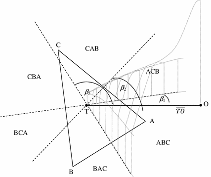
The division of the candidate plane into the six sectors that define the six rankings, and the volume of the wedge (the integral under the spherical bivariate normal distribution centered at \(O\)) that describes the probability that a randomly chosen voter ranks the three candidates in the order ABC
To match the variance of the angles that we determine from observed election data, we parameterize the Dirichlet distribution so that each of the three shares is multiplied by the common constant 73.5008. Dividing the three values in the text by this number yields three shares that sum to 1.
For example, if candidate \(A\) is the winner of voting situation \(R\), then the four pairs of rankings are (ABC, BAC), (ACB, CAB), (BAC, BCA), (CAB, CBA).
In three-candidate elections in which voters must submit full rankings, we treat a truncated ballot for candidate \(X\) as half a ballot for each of the two rankings with \(X \)first. This treatment permits us to examine truncated rankings with two rules, the Kemeny rule and the Coombs rule, that do not permit ballots listing only a single candidate.
The definition of SCC requires that the winner for \(R\) be the unique winner.

References
Arrow K (1951) Social choice and individual values, 1st edn. New York (2nd edn., New Haven, 1963)
Black D (1958) The theory of committees and elections. Cambridge University Press, Cambridge
Brams SJ (1982) The AMS nominating system is vulnerable to truncation of preferences. Not Am Math Soc 29:136–138
Chamberlin JR, Cohen M (1978) Toward applicable social choice theory: a comparison of social choice functions under spatial model assumptions. Am Polit Sci Rev 72:1341–1356
Chamberlin JR, Featherston F (1986) Selecting a voting system. J Polit 48(2):347–369
Condorcet MJAN (1785) “Essai sur l’application de l’analyse à la probabilité des décisions rendues à la pluralité des voix”. L’Imprimerie Royale, Paris
Coombs CH (1964) A theory of data. Wiley, New York
Copeland AH (1951) A ‘reasonable’ social welfare function”. Mimeo, University of Michigan, Department of Mathematics, Seminar on Applications of Mathematics to the Social Sciences
de Borda J-C (1784) Mémoire sur les élections au scrutin”. Histoire de l’Academie Royale des Sciences, Paris
Felsenthal DS (2012) Review of paradoxes afflicting procedures for electing a single candidate. In: Felsenthal DS, Machover M (eds) Electoral systems: paradoxes, assumptions, and procedures. Springer, Berlin, pp 19–91
Fishburn PC (1974a) Paradoxes of voting. Am Polit Sci Rev 68:537–546
Fishburn PC (1974b) On the sum-of-ranks winner when losers are removed. Discret Math 8:25–30
Fishburn PC (1977) Condorcet social choice functions. SIAM J Appl Math 33:469–489
Fishburn PC (1982) Monotonicity paradoxes in the theory of elections. Discret Appl Math 4:119–134
Fishburn PC, Brams SJ (1983) Paradoxes of preferential voting. Math Mag 56:207–214
Gehrlein W (2006) Condorcet’s paradox. Springer, Berlin
Gehrlein W, Lepelley D (2011) Voting paradoxes and group coherence: the Condorcet efficiency of voting rules. Springer, Berlin
Good IJ, Tideman TN (1976) From individual to collective ordering through multidimensional attribute space. Proc R Soc Lond Ser A 347:371–385
Henry M, Mourifié I (2011) Euclidean revealed preferences: testing the spatial voting model. J Appl Econ. doi:10.1002/jae.1276
Hoag CG, Hallett GH (1926) Proportional representation. Macmillan, New York
Kemeny J (1959) Mathematics without numbers. Daedalus 88:577–591
Laslier J-F (2011) Lessons from in situ tests during French elections. In: Dolez B, Grofman B, Laurent A (eds) In situ and laboratory experiments on electoral law reform: French presidential elections. Springer, Heidelberg, pp 90–104
Laslier J-F (2012) And the loser is plurality voting. In: Felsenthal DS, Machover M (eds) Electoral systems: paradoxes, assumptions, and procedures. Springer, Berlin, pp 327–351
Lepelley D, Merlin V (2001) Scoring run-off paradoxes for variable electo-rates. Econ Theory 17:53–80
Merrill S (1984) A comparison of efficiency of multicandidate electoral systems. Am J Polit Sci 28:23–48
Nanson E (1883) Methods of elections. Trans Proc R Soc Vic 19:197–240
Nurmi H (1992) An assessment of voting system simulations. Public Choice 73:459–487
Nurmi H (1999) Voting paradoxes and how to deal with them. Springer, Berlin
Nurmi H (2012) On the relevance of theoretical results to voting system choice. In: Felsenthal DS, Machover M (eds) Electoral systems: paradoxes, assumptions, and procedures. Springer, Berlin, pp 255–274
Plassmann F, Tideman TN (2011) How to assess the frequency of voting paradoxes and strategic voting opportunities in actual elections. Mimeo. Available at http://papers.ssrn.com/sol3/papers.cfm?abstract_id=1911286
Saari DG (2001) Decisions and elections; explaining the unexpected. Cambridge University Press, Cambridge
Smith JH (1973) Aggregation of preferences with variable electorate. Econometrica 41:1027–1041
Stern H (1993) Probability models on rankings and the electoral process. In: Flieger M, Verducci JS (eds) Probability models and statistical analysis for ranking data. Springer, Berlin, pp 173–195
Tideman TN (2006) Collective decisions and voting. Ashgate, Burlington
Tideman TN, Plassmann F (2012) Modeling the outcomes of vote-casting in actual elections. In: Felsenthal DS, Machover M (eds) Electoral systems: paradoxes, assumptions, and procedures. Springer, Berlin, pp 217–251
Young P (1974) An axiomatization of Borda’s rule. J Econ Theory 9:43–52
Young P (1988) condorcet’s theory of voting. Am Pol Sci Rev 82: 1231–1244
Acknowledgments
We thank two anonymous referees for their helpful comments and suggestions. All remaining errors are ours
Author information
Authors and Affiliations
Corresponding author
Appendices
Appendix 1: Simulating elections with the spatial model
1.1 A.1.1 A spatial model of vote-share probabilities
The spatial model of voting represents a conceptualization of the distribution of voter ideal points and the locations of candidates in candidate space. Good and Tideman (1976) describe the philosophy and the technical details of the spatial model that we use; here we summarize its essential elements. Consider the case of \(m\,=\,3\) candidates. There are two sub-cases to be considered. The first is that the three candidates are collinear, that is, all three lie in a single line. In this case, the candidate that is in the middle will not be the last choice of any voter. Since every candidate is the last choice of some voters in the vast preponderance of the results for elections with three candidates that we have seen, we neglect this case and consider the more general case in which the positions of three candidates are not collinear. In this case the locations of the three candidates define a plane, namely the plane that we call candidate space. Label the candidates \(A,\,B\), and \(C\), so that the 3! = 6 different strict rankings are ABC, ACB, CAB, CBA, BCA, and BAC. The six strict rankings form a voting situation that describes how many ballots voters have cast for each of the six rankings.
We assume that the locations of voter ideal points in candidate space follow a circularly symmetric bivariate normal distribution. The probability that a voter chosen at random will place the three candidates in a particular order (e.g., ABC) is the integral of the density function of voter ideal points over the portion of the plane where the order of the distances to the three candidates is the order prescribed by the ranking whose probability is being calculated. The portions of the plane assigned to the six rankings of the three candidates are delineated by the perpendicular bisectors of the line segments connecting pairs of candidates. Figure 3 shows, for specific locations of the three candidates, the division of the candidate plane into the six sectors that define the six rankings. The figure also shows the volume of the triangular wedge (the integral under the spherical multivariate normal distribution centered at \(O)\) whose integral describes the probability that a randomly chosen voter ranks the three candidates in the order ABC.Footnote 34
While there are six degrees of freedom in the locations of the three candidates, there are only four degrees of freedom in the probabilities determined by the integrals. One degree of freedom is lost because, if the positions of the three candidates are rotated around the mode of the distribution of voter ideal points, the pattern of perpendicular bisectors rotates by the same amount, and the integrals are unchanged. A second degree of freedom is lost because, if the locations of the three candidates are moved the same distance toward or away from the point that is equidistant from them, the perpendicular bisectors and hence the integrals are unchanged.
There are different ways to use the remaining four degrees of freedom to describe the structure of the spatial model. We found that the following parameterization makes it easiest to simulate rankings that are very similar to the voting situations that we observe in actual elections. We first place the intersection of the three perpendicular bisectors of the triangle formed by the three candidates (that is, the triangle’s circumcenter \(T\)) at the origin of a coordinate system, and we rotate the coordinate system so that the center of voter ideal points \(O\) is on its horizontal axis. We then use the first degree of freedom for the horizontal distance OT, and the remaining three degrees of freedom for the angles formed by the line \(\overline{OT}\) and the three perpendicular bisectors that describe the boundaries between pairs of the six strict rankings. To simulate data with the spatial model, we adopt distributions for the parameters based on the analysis of real voting data in Plassmann and Tideman (2011). In particular, we assume that \(\overline{OT}\) follows a Weibull distribution with scale parameter \(\alpha \,=\,0.6858\) and shape parameter \(\beta \,=\,2.4608\), and that the three angles follow a Dirichlet distribution with parameters \(\delta _{1}\,=\,26.47,\,\delta _{2}\, =\,23.37\), and \(\delta _{3}~=~23.65\).Footnote 35
1.2 A.1.2 A model of vote-casting outcomes
The spatial model yields a vote share probability \(p_{r}\) for each of the six strict rankings \(r\), with \(\Sigma p_{r}~=~1\). To complete the model of vote-casting, it is necessary to describe the relationship between the vote share probabilities (six real numbers) and the number of ballots that \(n\) voters submit for each of the six rankings (six integers). We assume that the \(p_{r}\)s represent the expected shares of the ballots. We also assume that the distribution of the vector of \(p_{r}\)s does not vary with the size of the electorate. To formalize these assumptions, let \(n_{r}\) be the number of ballots submitted for ranking \(r\), with \(\Sigma n_{r}=n\) and \(r=1,\ldots ,6\), and let \(N_{r}\) be a random variable that describes the distribution of \(n_{r}\). If voters cast their ballots independently of each other, then in a given election in which the expected vote shares are given by a vector of \(p_{r}\)s, the six \(N_{r}\)s follow a multinomial distribution with \(E[N_{r}]= np_{r}\) (and thus \(E[{N_r /n}]=p_r),\,Var[N_{r}]=np_{r}\,(1 - p_{r})\), and Cov [\(N_{r},\,N_{s}]=-np_{r}p_{s}\). One way of accommodating dependent ballots is to assume that the six \(n_{r}\)s follow a multinomial-Dirichlet distribution with \(E[N_{r}]=np_{r},\,Var[N_{r}]=np_{r}(1 - p_{r})\Psi \), and \(Cov[N_{r},\,N_{s}]=- np_{r}p_{s}\Psi \), where \(\Psi = (\psi +n)/(\psi + 1)\). The parameter \(\psi \) describes the additional variance that is introduced through the Dirichlet distribution; in the limit as \(\psi \) approaches infinity, the multinomial-Dirichlet distribution approaches the multinomial distribution. Plassmann and Tideman (2011) show that the multinomial distribution leads to less variation among simulated ballots than what is observed in ballots from actual elections, while the variation among ballots simulated with a multinomial-Dirichlet distribution with \(\psi ~=~330\) is very close to the variation among observed ballots. Thus a specified distribution for the \(p_{r}\)s leads to a distribution of election outcomes, for any size of electorate, that can be parameterized and simulated.
1.3 A.1.3 A model of voter behavior versus a model of vote-casting outcomes
The spatial model can be interpreted either as a model of voter behavior or as part of a model of vote-casting outcomes. It is important to distinguish the two interpretations. When viewed as a model of voter behavior, the task would be to identify the positions of the ideal points in actual elections. Knowledge of these positions would explain why one observes a particular voting situation. The key question would be whether observed voting situation can be interpreted as revealed preferences that provide information about the positions of the ideal points. This question has received considerable attention in the literature; Henry and Mourifié (2011) assess and reject the validity of the spatial model of voting when it is interpreted as a model of voter behavior.
In contrast, when the spatial model serves as a model of vote share probabilities and thus as part of a model of vote-casting outcomes, the focus is on the distribution of voting situations rather than the positions of ideal points. The task is to parameterize the spatial model so that the model of vote-casting outcomes yields a distribution of voting situations that corresponds to the distribution of observed voting situations. Knowledge of the positions of ideal points is not required for this task. Thus our work is neither related to nor affected by the literature on revealed preferences. We adopt the spatial model as a model of vote-casting outcomes solely because, among all contenders for a model of vote share probabilities of which we are aware, it comes closest to describing the distribution of observed voting situations, not because we want to defend it as a model of voter behavior.
Appendix 2: Estimating the frequencies of five voting paradoxes
Let “voting rule \(X\)” be the voting rule for which the frequency of occurrence of a paradox is to be determined. Let \(P\) be the number of occurrences of the paradox, where \(P\,=\,0\) before the first voting situation is drawn. Let \(N\) be the number of voting situations to be drawn.
1.1 A.2.1 The strong lack of monotonicity paradox
-
1.
Use the calibrated spatial model to draw a voting situation \(R\).
-
2.
Use voting rule \(X\) to determine the winner of \(R\).
-
3.
There are four pairs of rankings across which the winner is ranked in consecutive positions.Footnote 36 Consider each of these four pairs in turn, starting with the first pair. If the ranking in which the winner is ranked lower has at least one vote, then decrease the number of votes for that ranking by one and increase the number of votes for the other ranking by 1. Denote the new voting situation by \(R^\prime \). If the ranking in which the winner is ranked lower has no votes, then continue with the next pair of rankings. If this was the fourth pair of rankings, then continue with Step 1.
-
4.
Use voting rule \(X\) to determine the winner of \(R^\prime \).
-
5a.
(Ignoring ties) If voting rule \(X\) chooses different winners for \(R\) and \(R^\prime \), then increment \(P\) by 1. Continue with Step 1.
-
5b.
(Accounting for ties) If voting rule \(X\) chooses either (1) different winners for \(R\) and \(R^\prime \), or (2) the same winner for \(R\) and \(R^\prime \) and the winner is unique for \(R\) but not unique for \(R^\prime \), then increment \(P\) by 1. Continue with Step 1.
-
6.
If \(P\) was not incremented in Step 5, then the following must be true: voting rule \(X\) chooses the same winner for the two voting situations. Continue with Step 3 with a different pair of rankings. After the fourth pair, continue with Step 1.
-
7.
Determine the frequency of occurrence as \(P/N\).
1.2 A.2.2 The strong truncation paradox
Steps 1–2 and 4–7 are the same as in A.2.1
-
3.
Consider each of the six possible strict rankings in turn, starting with the first ranking. Denote this ranking by \(r\). If ranking \(r\) has at least one vote, then decrease the number of votes for ranking \(r\) by one-half. Identify the ranking \(r^\prime \) that has the same highest-ranked candidate as ranking \(r\), and increase the number of votes for ranking \(r^\prime \) by one-half.Footnote 37 Denote the new voting situation by \(R^\prime \). If ranking \(r\) has no votes, then continue with the next ranking. If ranking \(r\) is the sixth ranking, then continue with Step 1.
1.3 A.2.3 The strong no-show paradox
Steps 1–2 and 4–7 are the same as in A.2.1
-
3.
Consider each of the six possible strict rankings in turn, starting with the first ranking. Denote this ranking by \(r\). If ranking \(r\) has at least one vote, then decrease the number of votes for ranking \(r\) by one. Denote the new voting situation by \(R^\prime \). If ranking \(r\) has no votes, then continue with the next ranking. If ranking \(r\) is the sixth ranking, then continue with Step 1.
1.4 A.2.4 Violations of the Subset Choice Consistency (SCC) Condition
Steps 1–2 are the same as in A.2.1
-
3.
If the winner of voting situation \( R\) is not unique, then continue with Step 1.Footnote 38
-
4.
Consider, in turn, each of the two candidates who did not win, starting with the first of these candidates. Eliminate this candidate. Use \(R\) to assemble the voting situation \(R^{\mathrm{short}}\) for the ensuing two-candidate election.
-
5.
Use voting rule \(X\) to determine the winner for \(R^{\mathrm{short}}\) (this is the majority rule winner for all 14 voting rules that we consider).
-
6a.
(Ignoring ties) IF the winner for \(R^{\mathrm{short}}\) is not the same as the winner for \(R\), THEN increment \(P\) by 1. Continue with Step 1.
-
6b.
(Accounting for ties) IF (1) the winner for \(R^{\mathrm{short}}\) is not the same as the winner for \(R\), or (2) the winner for \(R^{\mathrm{short}}\) is not unique (there is a two way tie that involves the winner of \(R)\), THEN increment \(P\) by 1. Continue with Step 1.
-
7.
If \(P\) was not incremented in Step 6, then the following must be true: the winner for \(R^{\mathrm{short}}\) is the same as the winner for \(R\). Continue with Step 4 with the other candidate. After the second candidate, continue with Step 1.
-
8.
Determine the frequency of occurrence as \(P/N\).
1.5 A.2.5 The reinforcement paradox
We examine only the version of the reinforcement paradox for which the two elections under consideration either have the same number of voters or have a number of voters that differs by exactly 1 across the elections. When sampling the elections for the results reported in Table 12, we assumed that the number of voters in each of the two individual elections sum to the number of voters listed in the header of each column.
-
1.
Use the spatial model to draw two voting situations, \(R\) and \(R^\prime \).
-
2.
Use voting rule \(X\) to determine the winners for \(R\) and \(R^\prime \).
-
3.
If the winners of \(R\) and \(R^\prime \) are not the same, then continue with Step 1.
-
4.
Combine \(R\) and \(R^\prime \) to form a new voting situation \(R^{\prime \prime }\).
-
5.
Use voting rule \(X\) to determine the winner for \(R^{\prime \prime }\).
-
6.
EITHER the winners for \(R,\,R^\prime \), and \(R^{\prime \prime }\) are unique, OR some/all winners are not unique but one decides to ignore ties. One of the following must be true:
-
6a.
The winner for \(R^{\prime \prime }\) IS NOT the same as the winner for \(R\) and \(R^\prime \). If true, then increment \(P\) by 1 and continue with Step 1.
-
6b.
The winner for \(R^{\prime \prime }\) IS the same as the winner for \(R\) and \(R^\prime \). If true, then continue with Step 1.
-
6a.
-
7.
Reaching Step 7 implies that the winners for \(R,\,R^\prime \), and \(R^{\prime \prime }\) are not unique and that one decides not to ignore ties. One of the following must be true:
-
7a.
The winner of \(R^{\prime \prime }\) is tied with another candidate and the winners of \(R\) and/or \(R^\prime \) are tied with the same candidate. If true, then continue with Step 1.
-
7b.
The winner of \(R^{\prime \prime }\) is tied with another candidate and the winners of \(R\) and/or \(R^\prime \) are either not tied or tied with a different candidate. If true, then increment \(P\) by 1 and continue with Step 1.
-
7c.
The winner of \(R^{\prime \prime }\) is not tied and the winners of \(R\) and/or \(R^\prime \) are tied with another candidate. If true, then increment \(P\) by 1 and continue with Step 1.
-
7a.
-
8.
Determine the frequency of occurrence as \(P/N\).
Rights and permissions
About this article
Cite this article
Plassmann, F., Tideman, T.N. How frequently do different voting rules encounter voting paradoxes in three-candidate elections?. Soc Choice Welf 42, 31–75 (2014). https://doi.org/10.1007/s00355-013-0720-8
Received:
Accepted:
Published:
Issue Date:
DOI: https://doi.org/10.1007/s00355-013-0720-8