Büchi Store: an open repository of $\omega$-automata

Abstract

We introduce Büchi Store, an open repository of Büchi automata and other types of $\omega$-automata for model-checking practice, research, and education. The repository contains Büchi automata and their complements for common specification patterns and numerous temporal formulae. These automata are made as small as possible by various construction techniques in view of the fact that smaller automata are easier to understand and often help in speeding up the model-checking process. The repository is open, allowing the user to add automata that define new languages or are smaller than existing equivalent ones. Such a collection of Büchi automata is also useful as a benchmark for evaluating translation or complementation algorithms and as examples for studying Büchi automata and temporal logic. These apply analogously for other types of $\omega$-automata, including deterministic Büchi and deterministic parity automata, which are also collected in the repository. In particular, the use of smaller deterministic parity automata as an intermediary helps reduce the complexity of automatic synthesis of reactive systems from temporal specifications.

Appendices

Appendix A: $\omega$-Automata

$\omega$-Automata have essentially the same structure as classic finite-state automata, but operate on infinite words. An $\omega$-automaton accepts an infinite word if and only if there exists a run of the automaton on the word that follows some repetition patterns prescribed by the acceptance condition of the automaton. Formally, an $\omega$-automaton is a quintuple $\langle \varSigma , Q, \delta , q_0, Acc\rangle$:

• $\varSigma$ is the finite alphabet.

• $Q$ is the finite set of states.

• $\delta \subseteq Q \times \varSigma \times Q$ is the transition relation.

• $q_0 \in Q$ is the initial state.

• $Acc$ is the acceptance condition. Different acceptance conditions give rise to different types of $\omega$-automata.

The automata as defined are nondeterministic. An automaton is deterministic if, for all $a \in \varSigma$, $q_1, q_2, q_3 \in Q$, $(q_1,a,q_2) \in \delta$ and $(q_1,a,q_3) \in \delta$ imply $q_2 = q_3$ (as in classic automata). A run of an $\omega$-automaton on an infinite word $a_0a_1a_2\cdots \in \varSigma ^{\omega }$ is an infinite sequence of states $q_0q_1q_2\cdots \in Q^{\omega }$ such that, for every $i \ge 0$, $(q_i,a_i,q_{i+1}) \in \delta$. For a run $\rho$, let $\text{ inf}(\rho )$ denote the set of states that appear infinitely many times (or infinitely often) in $\rho$. Whether a run is considered accepting depends on the type of the $\omega$-automaton, which is determined by conditions in terms of $\text{ inf}(\rho )$ and $Acc$. An $\omega$-automaton accepts an infinite word if there is an accepting run of the automaton on the word. The set of words accepted by an $\omega$-automaton is called the language of the automaton or the language recognized by the automaton. In the following subsections, we introduce the common types of $\omega$-automata.

1.1 A.1 Büchi automata

Büchi automata are the most commonly used type of $\omega$-automata. The acceptance condition of a Büchi automaton is defined by a set of accepting states. A word is accepted by a Büchi automaton if and only if there exists a run of the automaton on the word that passes through at least one accepting state infinitely often. Formally, the acceptance condition of a Büchi automaton is a set $F\subseteq Q$. A run $\rho$ is accepting if $\text{ inf}(\rho ) \cap F \ne \emptyset$.

In Fig. 4 is a (nondeterministic) Büchi automaton intended for the property “eventually always $p$” (which cannot be specified by a deterministic Büchi automaton). Here, the alphabet is $\{\mathsf{p }, {\sim }\mathsf{p }\}$. The automaton accepts infinite words over $\{\mathsf{p }, {\sim }\mathsf{p }\}$ where from some point on $\mathsf p$ repeats indefinitely. The Büchi automaton in Fig. 5 is deterministic and accepts infinite words over $\{\mathsf{p }, {\sim }\mathsf{p }\}$ where ${\sim }\mathsf{p }$ occurs infinitely often (“infinitely often ${\sim }\mathsf{p }$”). The two Büchi automata are the complement of each other.

Fig. 4

A Büchi automaton for “eventually always $\mathsf p$”

Fig. 5

A Büchi automaton for “infinitely often $\mathsf {\sim }p$”

A generalization of Büchi automata, called generalized Büchi automata, allows multiple acceptance sets and is very useful as an intermediary in the translation from a temporal formula to a Büchi automaton. The acceptance condition of a generalized Büchi automaton is a set of acceptance sets $\{ F_1,F_2,\ldots ,F_m \}$, where $F_i \subseteq Q$. A word is accepted by a generalized Büchi automaton if and only if there exists a run of the automaton on the word that passes through each acceptance set infinitely often. In other words, a run $\rho$ is accepting if, for all $i$, $\text{ inf}(\rho )\cap F_i \ne \emptyset$.

Büchi and generalized Büchi automata are expressively equivalent and recognize $\omega$-regular languages (or regular $\omega$-languages), the infinite-word version of regular languages.

1.2 A.2 Other $\omega$-automata

We next introduce other common variants of $\omega$-automata, including co-Büchi, Muller, Rabin, Streett, and parity automata. All these variants of $\omega$-automata, except co-Büchi automata, define $\omega$-regular languages and are expressively equivalent to (nondeterministic) Büchi automata.

• co-Büchi automata: The acceptance condition is a set $F\subseteq Q$. A run $\rho$ is accepting if $\text{ inf}(\rho ) \cap F = \emptyset$.

• Muller automata: The acceptance condition is a set of acceptance sets $\mathcal F =\{F_1, F_2, \ldots , F_m\}$, where $F_i \subseteq Q$. A run $\rho$ is accepting if $\text{ inf}(\rho ) \in \mathcal F$.

• Rabin automata: The acceptance condition is a set of pairs of sets of states, called acceptance pairs, $\{(E_1,F_1),$ $(E_2,F_2), \ldots , (E_m,F_m)\}$, where $E_i, F_i \subseteq Q$. A run $\rho$ is accepting if, for some $i$, $\text{ inf}(\rho ) \cap E_i = \emptyset$ and $\text{ inf}(\rho ) \cap$ $F_i \ne \emptyset$.

• Streett automata: The acceptance condition , as in Rabin automata, is also a set of acceptance pairs $\{(E_1,F_1),$ $(E_2,F_2), \ldots , (E_m,F_m)\}$, where $E_i, F_i \subseteq Q$. A run $\rho$ is accepting if, for all $i$, $\text{ inf}(\rho ) \cap E_i \ne \emptyset$ or $\text{ inf}(\rho ) \cap F_i = \emptyset$.

• Parity automata: The acceptance condition is a mapping $c: Q \rightarrow \mathbb N$. A run $\rho$ is accepting if $\text{ min}\{c(q) \mid q\in \text{ inf}(\rho )\}$ is even.

Intuitively, a run is accepting in a co-Büchi automaton if it is eventually trapped outside of $F$ (or inside of $Q\setminus F$) and never returns to $F$. In Fig. 6 is a co-Büchi automaton for “eventually always $\mathsf p$”. Note that it is deterministic and recognizes the same language of the Büchi automaton in Fig. 4. It has exactly the same structure as the Büchi automaton in Fig. 5, which recognizes its complement “infinitely often $\mathsf {\sim }p$.”

Fig. 6

A co-Büchi automaton for “eventually always $\mathsf p$.” An accepting run must eventually be trapped outside of $\{s_0\}$, i.e., inside of $\{s_1\}$

A run of a Muller automaton is accepting if and only if the set of states visited infinitely often equals one of the acceptance sets. Given a Rabin acceptance pair $(E, F)$, set $E$ defines the set of states that should be visited only finitely many times while set $F$ defines the set of states that should be visited infinitely many times. An accepting run satisfies at least one of the Rabin acceptance pairs. The Streett acceptance condition is dual of the Rabin condition. A run is accepting in a Streett automaton if and only if it is not accepting in a Rabin automaton with the same structure and acceptance pairs. A parity automaton assumes each state has a parity number. A run of a parity automaton is accepting if and only if the smallest parity number that is visited infinitely often is even.

For further information, we refer the reader to the book by Grädel et al. [13].

B Linear temporal logic

1.1 B.1: PTL

Propositional (Linear) Temporal Logic (PTL) formulae are constructed by applying boolean and temporal operators to atomic propositions, or boolean variables, drawn from a predefined universe [20, 26]. Temporal operators are classified into future operators and past operators. Future operators include ${\bigcirc }$ (next), ${\Diamond }$ (eventually), ${\Box }$ (always), $\ \mathcal U \,$ (until), and $\ \mathcal W \,$ (wait-for); in some variant, $\ \mathcal R \,$ (release) is used in place of $\ \mathcal W \,$. Past operators include $\sim \!\!\!\!{\bigcirc }$ (before), ${-\!\!\!\!\!\!{\bigcirc }}$ (previous), ${}-\!\!\!\!{\Diamond }$ (once), ${{-\!\!\!\!{\Box }}}$ (so-far), $\ \mathcal S \,$ (since), and $\ \mathcal B \,$ (back-to); in the variant using $\ \mathcal R \,$, $\ \mathcal T \,$ (trigger) is used in place of $\ \mathcal B \,$.

Syntax: Let $V$ be a set of boolean variables. PTL formulae are defined inductively as follows:

• Every variable $p \in V$ is a PTL formula.

• If $f$ and $g$ are PTL formulae, then so are $\lnot f, f \vee g, f \wedge g, {\bigcirc }f, {\Diamond }f, {\Box }f, f\ \mathcal U \, g, f\ \mathcal W \, g, \sim \!\!\!\!{\bigcirc }f, {-\!\!\!\!\!\!{\bigcirc }}f, {}-\!\!\!\!{\Diamond }f, {{-\!\!\!\!{\Box }}}f,$ $f\ \mathcal S \, g$, and $f\ \mathcal B \, g$. ($\lnot f \vee g$ is also written as $f \rightarrow g$ and $(f \rightarrow g)\wedge (g\rightarrow f)$ as $f \leftrightarrow g$.)

The expressively equivalent subset of PTL without the past temporal operators is usually referred to as LTL in the model-checking community.

Semantics: A PTL formula is interpreted over an infinite sequence of states $\sigma =s_0s_1s_2\ldots$, relative to a position in that sequence. A state is a subset of $V$, containing exactly those variables that evaluate to true in that state. If each possible subset of $V$ is treated as a symbol, then a sequence of states can also be viewed as an infinite word over $2^V$. The semantics of PTL in terms of $(\sigma , i) \models f$ ($f$ holds at the $i$-th position of $\sigma$) is given below. We say that a sequence $\sigma$ satisfies a PTL formula $f$ or $\sigma$ is a model of $f$, denoted $\sigma \models f$, if $(\sigma ,0) \models f$. Two formulae $f$ and $g$ are equivalent if all models of $f$ are also models of $g$ and vice versa.

• For a boolean variable $p$,

  • $(\sigma ,i) \models p \iff p\in s_i$

• For boolean operators,

  • $(\sigma ,i) \models \lnot f \iff (\sigma , i) \models f$ does not hold

  • $(\sigma ,i) \models f \vee g \iff (\sigma , i) \models f$ or $(\sigma , i) \models g$

  • $(\sigma ,i) \models f \wedge g \iff (\sigma , i) \models f$ and $(\sigma , i) \models g$

• For future temporal operators,

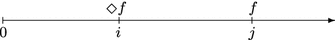
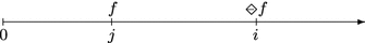
  • $(\sigma ,i) \models {\bigcirc }f\iff (\sigma , i+1) \models f$ That is, ${\bigcirc }f$ holds at position $i$ if and only if $f$ holds at position $i+1$, as visualized below.

    

  • $(\sigma ,i) \models {\Diamond }f \iff$ for some $j \ge i$, $(\sigma , j) \models f$ ${\Diamond }f$ holds at position $i$ if and only if $f$ holds at some position $j \ge i$.

    

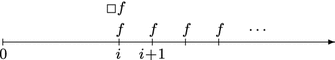
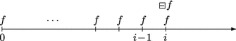
  • $(\sigma ,i) \models {\Box }f \iff$ for all $j \ge i$, $(\sigma , j) \models f$ ${\Box }f$ holds at position $i$ if and only if $f$ holds at every position $j \ge i$; note that $f$ also holds at position $i$.

    

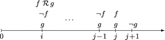
  • $(\sigma ,i) \models f\ \mathcal U \, g \iff$ for some $j \ge i$, $(\sigma , j) \models g$ and for all $k$, $i \le k < j$, $(\sigma , k) \models f$ $f\ \mathcal U \, g$ holds at position $i$ if and only if, for some $j\ge i$, $g$ holds at position $j$ and $f$ holds at every position $k$, $i \le k < j$.

    

  • $(\sigma ,i) \models f\ \mathcal W \, g \iff$ (for some $j \ge i$, $(\sigma ,j) \models g$ and for all $k$, $i \le k < j$, $(\sigma ,k) \models f$) or (for all $k \ge i$, $(\sigma ,k) \models f$) $f\ \mathcal W \, g$ holds at position $i$ if and only if $f\ \mathcal U \, g$ or ${\Box }f$ holds at position $i$.

  • When $\ \mathcal R \,$ is preferred over $\ \mathcal W \,$, $(\sigma ,i) \models f\ \mathcal R \, g$ $\iff$ for all $j\ge i$, if $(\sigma ,k) \not \models f$ for all $k$, $i\le k<j$, then $(\sigma ,j) \models g$.

    

• For past temporal operators,

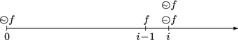
  • $(\sigma ,i) \models \sim \!\!\!\!{\bigcirc }f \iff i = 0$ or $(\sigma , i-1) \models f$

  • $(\sigma ,i) \models {-\!\!\!\!\!\!{\bigcirc }}f \iff i > 0$ and $(\sigma , i-1) \models f$ For $i>0$, $\sim \!\!\!\!{\bigcirc }f$ or ${-\!\!\!\!\!\!{\bigcirc }}f$ holds at position $i$ if and only if $f$ holds at position $i-1$. The difference between $\sim \!\!\!\!{\bigcirc }f$ and ${-\!\!\!\!\!\!{\bigcirc }}f$ occurs at position 0. $\sim \!\!\!\!{\bigcirc }f$ always holds at position 0, where ${-\!\!\!\!\!\!{\bigcirc }}f$ never holds.

    

  • $(\sigma ,i) \models {}-\!\!\!\!{\Diamond }f \iff$ for some $j$, $0 \le j \le i$, $(\sigma , j) \models f$ ${}-\!\!\!\!{\Diamond }f$ holds at position $i$ if and only if $f$ holds at some position $j$, $0 \le j \le i$.

    

  • $(\sigma ,i) \models {{-\!\!\!\!{\Box }}}f \iff$ for all $j$, $0 \le j \le i$, $(\sigma , j) \models f$ ${{-\!\!\!\!{\Box }}}f$ holds at position $i$ if and only if $f$ holds at every position $j$, $0 \le j \le i$.

    

  • $(\sigma ,i) \models f\ \mathcal S \, g \iff$ for some $j$, $0 \le j \le i$, $(\sigma ,j) \models g$ and for all $k$, $j < k \le i$, $(\sigma ,k) \models f$ $f\ \mathcal S \, g$ holds at position $i$ if and only if for some $j$, $0 \le j \le i$, $g$ holds at position $j$ and $f$ holds at every position $k$, $j < k \le i$.

    

  • $(\sigma ,i) \models f\ \mathcal B \, g \iff$ (for some $j$, $0\le j\le i$, $(\sigma ,j) \models g$ and for all $k$, $j < k \le i$, $(\sigma ,k) \models f$) or (for all $k$, $0\le k \le i$, $(\sigma ,k) \models f$) $f\ \mathcal B \, g$ holds at position $i$ if and only if $f\ \mathcal S \, g$ or ${{-\!\!\!\!{\Box }}}f$ holds at position $i$.

  • When $\ \mathcal T \,$ is preferred over $\ \mathcal B \,$ (because of $\ \mathcal R \,$ being preferred over $\ \mathcal W \,$), $(\sigma ,i) \models f\ \mathcal T \, g$ $\iff$ for all $j$, $0\le j \le i$, if $(\sigma ,k) \not \models f$ for all $k$, $j< k\le i$, then $(\sigma ,j) \models g$.

    

Table 5 Syntax for typing temporal formulae.

The language of the Büchi automaton in Fig. 4 is exactly the set of words/models satisfying ${\Diamond }{\Box }p$, while that of the automaton in Fig. 5 is exactly the set of words/models satisfying ${\Box }{\Diamond }\lnot p$. For every PTL formula, there is an equivalent Büchi automaton in sense that the Büchi automaton accepts precisely those words that are models of the PTL formula, but not vice versa. As an example, PTL is incapable of expressing “$p$ holds at every even position”; however, the corresponding language is Büchi-recognizable. $p\wedge {\Box }(p\rightarrow {\bigcirc }{\bigcirc }p)$ might look plausible, but is in fact too strict. (Note that positions in a sequence are numbered from $0$.) The formula requires that, once $p$ holds at some odd position, it must hold at all subsequent odd positions.

1.2 B.2: QPTL

Quantified propositional temporal logic (QPTL) [16, 26] is PTL extended with quantification over boolean variables (so, every PTL formula is also a QPTL formula):

• If $f$ is a QPTL formula and $x\in V$, then $\forall x\!:f$ and $\exists x\!:f$ are QPTL formulae.

Let $\sigma = s_0 s_1 \cdots$ and $\sigma ^{\prime } = s_0^{\prime } s_1^{\prime } \cdots$ be two sequences of states and $x$ an atomic proposition. We say that $\sigma ^{\prime }$ is a $x$-variant of $\sigma$ if, for every $i\ge 0$, $s_i^{\prime }$ differs from $s_i$ at most in the valuation of $x$, i.e., the symmetric set difference of $s_i^{\prime }$ and $s_i$ is either $\{x\}$ or empty. The semantics of QPTL is defined by extending that of PTL with additional semantic definitions for the quantifiers:

• For the quantifiers,

  • $(\sigma , i) \models \exists x\!:f \iff (\sigma ^{\prime }, i) \models f$ for some $x$-variant $\sigma ^{\prime }$ of $\sigma$

  • $(\sigma , i) \models \forall x\!:f \iff (\sigma ^{\prime }, i) \models f$ for every $x$-variant $\sigma ^{\prime }$ of $\sigma$

QPTL is expressively equivalent to Büchi automata. Let us examine a QPTL formula that specifies “$p$ holds at every even position” (which cannot be specified in PTL): $\exists t\!: (t \wedge {\Box }(t \leftrightarrow \lnot {\bigcirc }t) \wedge {\Box }(t \rightarrow p))$. Any sequence $\sigma$ that satisfies this formula has a $t$-variant $\sigma ^{\prime }$ satisfying $t \wedge {\Box }(t \leftrightarrow \lnot {\bigcirc }t) \wedge {\Box }(t \rightarrow p)$. From $t \wedge {\Box }(t \leftrightarrow \lnot {\bigcirc }t)$, we can infer that $t$ holds at every even position but does not hold at any odd position along $\sigma ^{\prime }$. The fact that $t$ holds at every even position and $\sigma ^{\prime }$ satisfies ${\Box }(t \rightarrow p)$ forces $p$ to hold at every even position in $\sigma ^{\prime }$. Since the two sequences $\sigma$ and $\sigma ^{\prime }$ are a $t$-variant of each other, $p$ also holds at every even position in $\sigma$. No restrictions on $p$ are imposed at odd positions, however. The variable $t$ does not hold at any odd position, so $p$ may or may not hold at odd positions in $\sigma ^{\prime }$ and hence in $\sigma$.

C Screen shots from Büchi Store

First of all, we note that, for the textual representation of boolean connectives and temporal operators, Büchi Store follows the format as used in the GOAL tool [33], shown in Table 5. The same holds for the alphabet of an automaton. A typical alphabet $\{\mathsf{pq }, \mathsf{p }{\sim }\mathsf{q }, {\sim }\mathsf{pq },{\sim }\mathsf{p }{\sim }\mathsf{q }\}$ represents $2^{\{\mathsf{p,q }\}}$; $\mathsf p$ appearing alone in a transition means either $\mathsf pq$ or $\mathsf p {\sim }\mathsf q$.

Figure 7 shows the browsing of automata in the Store with a particular setting of the sort and filter options. Each filter option includes quite a few possible values to select from and a “Select/Deselect All” switch is provided. To select $1$ and $2$ for the state size as in Fig. 7, the user can click on Deselect All and then check the two corresponding boxes. Each entry in the returned results shows the formulae that are equivalent to (but syntactically different from) the formula specifying the entry and also the formulae that identify its (semantic) complement.

Fig. 7

Browsing automata in the Store. The “State Size” filter option is set to select automata with one or two states, while the corresponding sort key is set to view the selected automata in decreasing order of state size

Figure 8 shows a failed attempt of uploading a Büchi automaton for ${\Box }(p\rightarrow p\ \mathcal U \, q))$ because the uploaded automaton is incorrect. The Store is also capable of determining if an uploaded automaton is structurally identical (isomorphic) to an existing one in the Store, in which case the uploaded automaton will be discarded.

Fig. 8

A failed attempt of uploading a Büchi automaton. The response from the Store on the right indicates that the uploaded automaton is incorrect. (Note: the path of the uploaded automaton displayed prior to the response in the “Automaton file” field has been cleared)

References

Boker, U., Kupferman, O.: Co-ing Büchi made tight and useful. In: Proceedings of the 24th annual IEEE symposium on logic in computer science (LICS ’09), pp. 245–254. IEEE Computer Society (2009)
Büchi J.R.: On a decision method in restricted second-order arithmetic. In: Proceedings of the 1960 international congress on logic, methodology and, philosophy of science, pp. 1–11 (1962)
Chatterjee, K., Henzinger, T.A., Jobstmann, B., Singh, R.: QUASY: Quantitative synthesis tool. In: Proceedings of the 17th international conference on tools and algorithms for the construction and analysis of systems (TACAS ’11), LNCS 6605, pp. 267–271. Springer, Heidelberg (2011)
Cichoń J., Czubak A., Jasiński A.: Minimal Büchi automata for certain classes of LTL formulas. In: Proceedings of the fourth international conference on dependability of computer systems, pp. 17–24. IEEE (2009)
CodeIgniter. http://codeigniter.com/
Couvreur, J.M.: On-the-fly verification of linear temporal logic. In: World Congress on formal methods in the development of computing systems (FM ’99), LNCS 1708, pp. 253–271. Springer, Heidelberg (1999)
Daniele, M., Giunchiglia, F., Vardi, M.Y.: Improved automata generation for linear temporal logic. In: Proceedings of the 11th international conference on computer-aided verification (CAV ’99), LNCS 1633, pp. 249–260. Springer, Heidelberg (1999)
Dwyer, M.B., Avrunin, G.S., Corbett, J.C.: Patterns in property specifications for finite-state verification. In: Proceedings of the 21st international conference on software engineering (ICSE ’99), pp. 411–420 (1999)
Etessami K., Holzmann G.J.: Optimizing Büchi automata. In: Proceedings of the 11th international conference on concurrency theory (CONCUR ’00), LNCS 1877, pp. 153–167. Springer, Heidelberg (2000)
Gastin, P., Oddoux, D.: LTL 2 BA: fast translation from LTL formulae to Büchi automata. http://www.lsv.ens-cachan.fr/gastin/
Gastin P., Oddoux D.: Fast LTL to Büchi automata translation. In: Proceedings of the 13th international conference on computer-aided verification (CAV ’01), LNCS 2102, pp. 53–65. Springer, Heidelberg (2001)
Giannakopoulou D., Lerda F.: From states to transitions: improving translation of LTL formulae to Büchi automata. In: Proceedings of the IFIP WG 6.1 international conference on formal techniques for networked and distributed sytems (FORTE ’02), LNCS 2529, pp. 308–326. Springer, Heidelberg (2002)
Grädel, E., Thomas, W., Wilke, T.: Automata, logics, and infinite games (LNCS 2500). Springer, Heidelberg (2002)
Holzmann, G.J.: The SPIN model checker: primer and reference manual. Addison-Wesley, Boston (2003)
Kähler, D., Wilke, T.: Complementation, disambiguation, and determinization of Büchi automata unified. In: Proceedings of the 35th international colloqium on automata, languages, and programming (ICALP ’08), LNCS 5125, pp. 724–735. Springer, Heidelberg (2008)
Kesten, Y., Pnueli, A.: Complete proof system for QPTL. J. Logic Comput. 12(5), 701–745 (2002)
Kupferman, O., Vardi, M.Y.: Weak alternating automata are not that weak. ACM Trans. Comput. Logic 2(3), 408–429 (2001)
Landweber, L.H.: Decision problems for \(\omega \)-automata. Math. Syst. Theory 3(4), 376–384 (1969)
Manna, Z., Pnueli, A.: A hierarchy of temporal properties. In: Proceedings of the 9th ACM symposium on principles of distributed computing (PODC ’90), pp. 377–408. ACM (1990)
Manna, Z., Pnueli, A.: The temporal logic of reactive and concurrent systems: specification. Springer, Heidelberg (1992)
Michel, M.: Complementation is more difficult with automata on infinite words. In: CNET, Paris (1988)
PHP/Java Bridge. http://php-java-bridge.sourceforge.net/
Piterman, N.: From nondeterministic Büchi and Streett automata to deterministic parity automata. In: Proceedings of the 21th annual IEEE symposium on logic in computer science (LICS ’06), pp. 255–264. IEEE (2006)
Safra, S.: On the complexity of \(\omega \)-automta. In: Proceedings of the 29th annual IEEE symposium on foundations of computer science (FOCS ’88), pp. 319–327. IEEE (1988)
Schewe, S.: Büchi complementation made tight. In: Proceedings of the 26th international symposium on theoretical aspects of computer science (STACS ’09), LIPIcs 3 Schloss Dagstuhl - Leibniz-Zentrum fuer Informatik, pp. 661–672 (2009)
Sistla, A.P.: Theoretical issues in the design and verification of distributed systems. PhD thesis, Harvard (1983)
Sistla, A.P., Vardi, M.Y., Wolper, P.: The complementation problem for Büchi automata with applications to temporal logic. Theo. Comp. Sci. 49, 217–237 (1987)
Sohail, S., Somenzi, F., Ravi, K.: A hybrid algorithm for LTL games. In Proceedings of the 9th international conference on verification, model checking, and abstract interpretation (VMCAI ’08), LNCS 4905, pp. 309–323. Springer, Heidelberg (2008)
Somenzi, F., Bloem, R.: Efficient Büchi automata from LTL formulae. In Proceedings of the 12th international conference on computer-aided verification (CAV ’00), LNCS 1855, pp. 248–263. Springer, Heidelberg (2000)
The Spec Patterns Repository. http://patterns.projects.cis.ksu.edu/
Tomcat. http://tomcat.apache.org/
Tsai, M.-H., Fogarty, S., Vardi, M.Y., Tsay, Y.-K.: State of Büchi complementation. In: Proceedings of the 15th international conference on implementation and application of automata (CIAA ’10), LNCS 6482, pp. 261–271. Springer, Heidelberg (2011)
Tsay, Y.-K., Chen, Y.-F., Tsai, M.-H., Chan, W.-C., Luo, C.-J.: GOAL extended: towards a research tool for omega-automata and temporal logic. In: Proceedings of the 14th international conference on tools and algorithms for the construction and analysis of systems (TACAS ’08), LNCS 4963, pp. 346–350. Springer, Heidelberg (2008)
Tsay, Y.-K., Tsai, M.-H., Chang, J.-S., Chang, Y.-W.: Büchi Store: an open repository of Büchi automata. In: Proceedings of the 17th international conference on tools and algorithms for the construction and analysis of systems (TACAS ’11), LNCS 6605, pp. 262–266. Springer, Heidelberg, (2011)
Vardi, M.Y., Wolper, P.: An automata-theoretic approach to automatic program verification. In: Proceedings of the 1st annual IEEE symposium on logic in computer science (LICS ’86), pp. 332–344. IEEE (1986)
Acknowledgments
This work was supported in part by National Science Council, Taiwan, under the grant NSC97-2221-E-002-074-My3. We thank Moshe Vardi and Wolfgang Thomas for teaching us so much about \(\omega \)-automata. Moshe’s enthusiasm in pursuing the automata-theoretic approach to model checking was a great source of inspiration for us to create Büchi Store. The diagram depicting the Temporal Hierarchy was learned from Wolfgang while he explained to us the use of DBW and DCW in the classification. Moshe’s Ph.D. student Seth Fogarty, during his visit to our group in the summer of 2009, witnessed the initiation of Büchi Store and made several useful comments. We thank Barbara Jobstmann whose suggestion of including deterministic parity automata prompted us to expand the Store to its current scope. The idea of maintaining a containment partial order of the language-equivalence classes should be shared with a participant of ETAPS 2011 whose name we could not recall; we thank him as well. Finally, we thank the three anonymous reviewers whose constructive and very detailed comments have helped improve the paper tremendously.
Author information
Authors and Affiliations
Corresponding author
Additional information
A preliminary version under a slightly different title “Büchi Store: An Open Repository of Büchi Automata” appeared in TACAS 2011 [34]. The third author Jinn-Shu Chang is now with Chunghwa Telecom and the fourth author Yi-Wen Chang is now with TSMC. Their contributions to this work were completed while they were graduate students at National Taiwan University.