Integrating the DEMATEL with the analytic network process for effective decision-making

Abstract

One of the most advanced and complex multi-criteria decision-making methods is the analytic network process (ANP). This method supports modelling dependencies and feedback between elements in the network, while most other methods do not support this feature. For this reason, the ANP is one of the most appropriate methods for making decisions in the fields characterised by existing dependencies of higher-level elements on lower-level elements, such as the higher education field. However, the implementation of the ANP can be problematic, as it is characterised by highly complex and time-consuming processes, and users’ occasional misunderstandings of some ANP steps. Also, conducting the ANP requires a specific decision-making problem structure, which is a cluster-node structure in the form of a network. To assist with problem structuring and decrease some of the problematic ANP implementation characteristics, specific methods, such as the decision-making trial and evaluation laboratory (DEMATEL) and interpretative structural modelling, have been chosen and integrated with the ANP. This paper focuses on the integration and analysis of the DEMATEL with the ANP. A literature review of how these two methods have been used together is given. Additionally, a new way of integrating these two methods (with two variants) is proposed and evaluated. According to the survey results, new ways of integrating the ANP and the DEMATEL decrease the complexity of the decision-making process, reduce the duration of the decision-making process, and increase users’ understanding of the method. The research methodology used in this paper is the design science research process.

1 Introduction

Many methods can be used for multi-criteria decision making (MCDM), but the most well-known method is the analytic hierarchy process (AHP). In the AHP, the decision-making problem is decomposed into a hierarchy. At the top of the hierarchy is the decision-making goal. The criteria are on the next level and can be decomposed into the sub-criteria (and further decomposed to the lower levels). On the last level are the alternatives. By using pairwise comparisons, local priorities of alternatives as well as criteria weights are calculated (Kadoić et al. 2017b). Then, it is possible to calculate the total priorities of alternatives and make decision (Saaty 2008).

The meaning of the concept ‘depend on’ is the opposite of ‘have an influence on’. Examples of concepts of influences and dependencies: the quality of the product influences the price of the product (the price of the product depends on the quality of the product); the motivation of employee influences the productivity of the employee (the productivity of the employee depends on his/he motivation).

When the influences between criteria are examined (Fig. 1b), the direct connection from criterion 1 to criterion 3 contributes to increasing the weight of criterion 1 and to decreasing the weight of criterion 2, when compared to Fig. 1a.

Fig. 1

a Decision-making criteria without influences between them and b decision-making criteria with influences between them

In the decision-making problem field, if influences/dependencies exist between criteria (see Fig. 1b), which the AHP does not consider, using the AHP might lead to a decision that is less than optimal (Kadoić et al. 2017b). In such cases, using the analytic network process (ANP) is more appropriate. By using the ANP, we can model the dependencies and feedback between the decision-making elements (Saaty 2001), and calculate more precise weights of the criteria as well as the local and global priorities of alternatives. Some other methods that can be used in fields characterised by the existence of influences (dependencies) between criteria include the weighted influence non-linear gauge system (WINGS; Michnik 2013) and social network analitic process SNAP (Kadoić et al. 2017a).

To be able to apply a decision-making method that supports including influences between criteria in the calculation of the criteria weights, the specific structure of the decision-making problem is required. This structure is a network consisting of nodes that represent criteria, and which can be grouped into clusters, and connections that represent influences between the criteria. In terms of graph theory, this network is an unweighted directed graph in the case of the ANP, and a weighted directed graph in the case of WINGS or SNAP. The structuring methods that can assist with the decision-making problem structuring procedure are the top-down and bottom-up approaches (Kadoić et al. 2017c), the PrOACT approach (Hammond et al. 1999), interpretative structural modelling [ISM; examples are given in Attri et al. (2013)] and the decision-making trial and evaluation laboratory (DEMATEL) [examples are given in Sumrit and Anuntavoranich (2013)].

In this paper, we first present the research methodology and the objectives (Sect. 2). In Sect. 3, we describe the ANP method, and address some weaknesses of the method based on a literature review and our experience. In terms of structuring methods, we focus on and describe the DEMATEL (Sect. 4) and review some of the literature on using ANP together with DEMATEL (Sect. 5.1). In Sect. 5.2, we propose some upgrades of the DEMATEL–ANP that make integrating DEMATEL and ANP more efficient. In Sect. 6, we describe how proposed upgrades are evaluated and present the results of the evaluation.

2 Research methodology and paper objectives

According to the types of research designs (Creswell 2009), the design of this research is mixed method research. It is a pragmatic research philosophy, and the research methodology follows the design science research process (DSRP). The phases of this research, adapted from Peffers et al. (2006) and Vaishnavi and Kuechler (2004), are:

• 1. Problem identification and motivation The field of higher education (HE) is characterised by existing dependencies and influences between criteria in decision-making problems. Some of the methods that support modelling dependencies between criteria are the ANP (Saaty 2001) and the WINGS (Michnik 2013). As concluded in literature review analysis in Kadoić et al. (2016), the AHP is the most often used in practice of strategic decision making in HE. By including dependencies between criteria, we obtain more accurate criteria weights (Begičević 2008). The ANP is often avoided because of its complexity. However, when it is used, it is often applied in conjunction with another method, thereby diminishing some of its weak points. The DEMATEL is one method that can be integrated with the ANP. This phase is related to the first objective of this paper (see below), which corresponds to Sects. 3 and 4.

• 2. Objectives of the solution In this phase, variables that describe the implementation complexity of DEMATEL–ANP will be examined. The focus is on input data that need to be obtained by the decision-making user. This phase is related to the second objective of the paper (see below), which corresponds to Sect. 5.1.

• 3. Design and development A new artefact, i.e. a new DEMATEL–ANP approach, will be defined and presented in this phase. This phase is related to the third objective of this paper (see below), which corresponds to Sect. 5.2.

• 4. Demonstration of the artefact The new DEMATEL–ANP approach will be implemented in a case from the area of higher education, the evaluation of candidates for the assistant professor position. This phase is related to the fourth objective of this paper (see below) which corresponds to Sect. 6.2.

• 5. Evaluation of the artefact The newly developed DEMATEL–ANP approach will be compared to the DEMATEL–ANP approaches currently in use from a theoretical and practical points of view (Sect. 5.2.). This phase is related to the fifth and sixth objectives of this paper (see below) and corresponds to Sects. 6.1 and 6.3.

• 6. Dissemination phase This paper is currently the main way to disseminate the results of this research. However, this research will be continued in the future, and those results will be disseminated.

The objectives of the research are:

• 1. To present and analyse the characteristics of the ANP and the DEMATEL;

• 2. To analyse current integrations of the DEMATEL and the ANP;

• 3. To develop and present a new DEMATEL–ANP integration approach;

• 4. To demonstrate a new integration approach on a real case example;

• 5. To analyse a new integration approach and compare it to current integration approaches on a theoretical level; and

• 6. To compare the implementation results of a new approach with the implementation results of a ‘clean’ ANP and some of the current DEMATEL–ANP approaches.

3 The analytic network process (ANP)

The decision-making problems in the ANP are modelled as networks, not as hierarchies as with the AHP. The ANP is a generalisation of the AHP. The basic elements in the hierarchy and network are clusters, nodes and dependencies (arcs).

The steps of the ANP (Begičević 2008; Saaty and Cillo 2008) can be described through a simple example, evaluation of senior researchers (scientists). Senior researchers are active in both the research and teaching fields. To make the further analysis easier, we bring the ANP analysis of this decision-making problem that is already presented in Kadoić et al. (2017a).

Problem structuring The goal of the decision-making is to select the best scientists among three scientists. This means that we will have: (1) cluster Goal with node G; (2) clusters Alternatives with three nodes, alternatives A1, A2 and A3; and (3) five nodes of criteria (papers—pa, citations—ci, projects—pr, courseware—co, grades from students—gr) grouped into two clusters (Science—first three criteria and Teaching—last two criteria). The problem structure is shown in Fig. 2. Solid arcs (arrows) are related to the dependencies of the goal on criteria. Dashed arcs are related to the dependencies between criteria. Dotted arcs are related to the dependencies of alternatives on criteria and dependencies of criteria on alternatives. Arcs between alternatives and criteria, pa and co, are not shown because of the complexity of the figure, but those dependencies also exist. The decision-making structure can be shown in a simpler way (with information lost; see Fig. 3). The Goal is a source cluster that depends on Science and Teaching. The other three clusters are intermediate components. The dashed arc between Science and Teaching is the result of the existence of at least one arc between at least one criterion from Science and at least one criterion in Teaching, e.g. pr depends on co. The dashed arc between Teaching and Science can be interpreted similarly. The loops in the clusters Science and Teaching are the result of the existence of at least one dependency of one criterion on another in the same cluster, e.g. ci depends on pa, or gr depends on co.

Fig. 2

Structure of problem ‘evaluation of scientists’—node level

Fig. 3

Structure of problem ‘evaluation of scientists’—cluster level

Pairwise comparisons on the node level Now, we should create the unweighted supermatrix. It is a square matrix of all nodes in the decision-making problem and contains local priorities. When making judgements in pairwise comparisons, we use Saaty’s fundamental scale of absolute numbers (Saaty 2008), just as with the AHP. To fill the unweighted supermatrix (Table 1) with priorities, we have to make pairwise comparisons of nodes with respect to other nodes. The comparisons that have to be done are:

Table 1 Unweighted supermatrix

• Comparisons of the criteria with respect to the goal (solid arcs in Fig. 2): comparisons of criteria in Science with respect to G (local priorities will be put into the supermatrix at rows ci, pr, pa and column G); comparisons of criteria in Teaching with respect to G (local priorities will be put at rows co, gr and column G).

• Comparisons of criteria with respect to other criteria—comparisons of the criteria that leave (influence) the same criterion from the same cluster with respect to it (dashed arcs in Fig. 2): pa and pr with respect to ci; pa and ci with respect to pr. Priorities are put into the supermatrix depending on which criteria (rows) influence which criterion (column). When making a pairwise comparison between pa and pr with respect to ci, we try to answer the question, ‘Which criterion, pa or pr, has a higher influence on criterion ci, and by how much?’ When some criteria depend on only one criterion in the same cluster, we do not make a comparison, and write 1 in the related cell in the supermatrix, e.g. cell (pr, pa) = 1;

• Comparisons of alternatives with respect to each criterion (see dotted arcs from criteria to alternatives in Fig. 2), the same as in the AHP. This will fill part of the supermatrix as follows: rows A1, A2 and A3, columns co, gr, pa, ci, pr;

• Comparisons of criteria in each cluster with respect to each alternative (see the dotted arc from alternatives to criteria in Fig. 2). This will fill part of the supermatrix as follows: rows co, gr, pa, ci, pr, columns A1, A2 and A3. For example, let us say that alternative A1 has a good value in terms of criterion co, and a very bad value in terms of gr. Let us use 4 on Saaty’s scale to describe this importance; then, at column A1, in rows co and gr, we will write 0.2 and 0.8, respectively.

Pairwise comparisons on a cluster level The goal of this step is to convert the unweighted matrix into the weighted supermatrix (Table 2). For this, we have to do the following comparisons:

Table 2 Weighted supermatrix

• Compare two clusters of criteria with respect to the Goal. For example, if we say that cluster Science is more important than Teaching, 3 in Saaty’s scale, by using the same pairwise comparisons procedure as when comparing the nodes, we will get weights 0.25 (Teaching) and 0.75 (Science). This means that 0.25 will multiply Teaching’s criteria and 0.75 will multiply Science’s criteria in column G;

• Compare clusters Teaching, Science and Alternatives with respect to Teaching. In this example, Teaching is equally important as Science with respect to Teaching, and Alternatives are three times more important than Teaching and Science. The priorities are: 0.2, 0.2 and 0.6, respectively;

• Compare clusters Teaching, Science and Alternatives with respect to Science. In this example, Teaching is equally important as Science with respect to Science, and Alternatives are three times more important than Teaching and Science. The priorities are: 0.2, 0.2 and 0.6, respectively.

• Compare clusters Teaching and Science with respect to Alternatives. In this example, they are equally important.

Calculating the limit matrix In this step, the weighted matrix is multiplied by itself as long as all of its columns become equal. This is how we get the final priorities.

Sensitivity analysis This is the last step in the ANP. The main idea of sensitivity analysis is to determine the influence of (small) changes of ANP inputs (pairwise comparisons, dependencies) on the final decision, ranks or priorities. Sensitivity analysis is currently not the focus of our research.

In terms of software support, the Creative Decisions Foundation’s Super Decisions (webpage: https://www.superdecisions.com) supports all the math behind the ANP.

The field of higher education is characterised by existing dependencies between criteria and feedback in decision-making problems. However, the literature review about which decision-making methods have been used in practice to solve problems showed that the AHP method was used more often than the ANP (Kadoić et al. 2016). The weaknesses of the ANP are related to the complexity of the method, the duration of implementation, and uncertainty in giving judgements, especially those on the cluster level (Kadoić et al. 2017d). Therefore, we can conclude that integrating the ANP with some other method(s) with the aim of eliminating its recognised disadvantages is welcome.

4 The decision-making trial and evaluation laboratory (DEMATEL)

The DEMATEL was developed between 1972 and 1979 with the aim of studying and analysing complex intertwined groups. It has been widely accepted as one of the best methods for modelling influences between components. In the decision-making field, it is used to form and then analyse relationships between criteria (Sumrit and Anuntavoranich 2013). The main steps of the DEMATEL are as follows (Chang et al. 2011; Michnik 2013; Ölçer 2013; Sumrit and Anuntavoranich 2013):

• 1. Data are collected from experts and matrix $Z$ is filled. The size of matrix $Z$ is $\left( {n, n} \right)$ where n is the number of criteria. For each expert, his/her matrix of influences is created, $X^{i} {-} X^{1} , X^{2} , \ldots , X^{m}$, where $m$ is a number of experts who make judgements. The scale that is used consists of five degrees: 0 (no influence between criteria); 1 (low influence between criteria); 2 (medium influence between criteria); 3 (strong influence between criteria); and 4 (very strong influence between criteria). Matrix $Z$ is calculated according to the next equation:

  $$ Z = \left[ {z_{ij} } \right];\, z_{ij} = \frac{1}{m}\mathop \sum \limits_{k = 1}^{m} x_{ij}^{k} $$

  (1)

• 2. In the second step, a normalised initial matrix of connection $D$ is calculated. To calculate this matrix, the values in matrix $Z$ are divided by the maximum sum of all rows and columns.

• 3. Calculation of the total matrix of connection $T.$$T$ is calculated using the Eqs. 2 and 3 (I is the identity matrix):

  $$ T = { \lim }_{m \to \infty } \left( {D^{1} + D^{2} + D^{3} + \cdots + D^{m} } \right) $$

  (2)
  $$ T = D\left( {I - D} \right)^{ - 1} $$

  (3)

• 4. In $T$, sums of rows and columns have to be calculated. The sum of a specific row ($r_{i}$) presents the total influence of an criterion on other criteria, and the sum of a certain column ($c_{i}$) represents the total influence of all other criteria on the criterion.

• 5. For each criterion, it is possible to calculate two values: $\left( {r_{i} + c_{i} } \right)$—the sum of influences of a certain criterion on others and dependencies of a certain criterion on others; and $\left( {r_{i} - c_{i} } \right)$—the difference between influences and dependencies of a certain criterion on others. When $\left( {r_{i} - c_{i} } \right)$ is positive, the criterion can be called ‘source’ in a network, and when $\left( {r_{i} - c_{i} } \right)$ is negative, the criterion is called ‘sink’ or ‘receiver’ in the network.

• 6. Calculation of the threshold value Alpha ($\alpha$). If the value in a certain cell $\left( {x, y} \right)$ in matrix $T$ is lower than $\alpha$, then we conclude that criterion $x$ does not influence $y$. Similarly, if the value in cell $\left( {x, y} \right)$ in matrix $T$ is higher than $\alpha$, then we conclude that $x$ influences $y$. There is a discussion on how to determine the size of the $\alpha$ threshold. In most cases, it is suggested to calculate $\alpha$ as the arithmetic mean of all values in matrix $T$. In this paper, we do not discuss in detail effects of different approaches of $\alpha$ determination on the finale results. Each approach influences the final solution differently.

• 7. Creation of a network relationship map (NRM). We plot a 2D coordinate system. One axis is $\left( {r_{i} + c_{i} } \right)$ and the other is $\left( {r_{i} - c_{i} } \right)$. We put all criteria in a coordinate system according to their values calculated in step 5. Additionally, we plot the connections between criteria respecting step 6.

In the case of evaluating scientists, the DEMATEL has been conducted before the ANP, and the ANP structure presented in Fig. 2 is a result of applying the DEMATEL. The original matrix $Z$ for this specific case is given in Table 3. The total matrix of connection $T$ is given in Table 4. The threshold value $\alpha$ is calculated by the arithmetic mean in matrix $T$.

Table 3 Matrix $Z$—influences between criteria

Table 4 Total matrix of connection $T$($\alpha$ = 0.58273)

The bold values in $T$ are associated with the ‘strongest’ influences in the decision-making problem; they are higher than $\alpha$ (values on the main diagonal are not observed). Since in the ANP we model dependencies, we have just ‘read’ matrix $T$ and can easily create connections in the ANP. The first bold value is (co, gr), which means that co influences gr (and gr is dependent on co); then we have to create a connection from gr to co. Similarly, all other connections in Fig. 2 are created.

We conclude that there are main benefits from the DEMATEL as follows (Shao et al. 2014):

• Standardised DEMATEL scale for determining influences between criteria.

• ‘Filter’ of the ‘strongest’ values (Step 6), which is very interesting in terms of the ANP. One of the main ideas of integrating the ANP and the DEMATEL is that with an initial number of connections between criteria (influences), we decrease to the strongest connections. As mentioned earlier, two of the main weak points of the ANP from a position of method implementation is the duration of the process and the substantial number of pairwise comparisons that need to be done. By decreasing the number of influences (dependencies) between criteria, we significantly decrease the number of comparisons that have to be implemented. Still, sometimes conducting the DEMATEL does not decrease the number of connections between criteria (without adjusting the $\alpha$).

• Values $\left( {r_{i} + c_{i} } \right)$ and $\left( {r_{i} - c_{i} } \right)$ give us the first information about the criteria weights which can, be included in inconsistency measures in the ANP.

5 Integrating the ANP and the dematel

5.1 State of the art

The previous section presented one of the potential benefits of integrating the ANP and the DEMATEL, namely decreasing the complexity of the network structure, which also simplifies implementation of the ANP. An example of this type of integration is given in Shih-Hsi et al. (2012). Lu and Lin (2010) also combined the DEMATEL and the ANP into a hybrid MCDM model to construct a green innovation strategic model. Here, the DEMATEL was used to acquire the structure of the MCDM problems, and the ANP was used to obtain the weights of each criterion. A second example of integrating the ANP and the DEMATEL is presented in a paper by Yang et al. (2008). In this paper, the DEMATEL was also used to create the network structure, but in this case, the DEMATEL played an additional role in the integration. It was used in the process of obtaining the weighted supermatrix in the ANP. The unweighted matrix from the previous ANP step was multiplied with a normalised α-cut total-influence matrix $\varvec{T}$. Essentially the same integration concept was used in two other papers (Ou Yang et al. 2013; Yang and Tzeng 2011). The DEMATEL was used in both segments: structuring the problem and obtaining the weighted supermatrix. Very similar role of the DEMATEL in a DEMATEL–ANP integration is presented in Ölçer (2013). The author created a software called TEMPOS, which supports this integration in Excel. The purpose of the research was to develop a decision support system to guide contractors in the decision-making for international projects. The name of the software is related to six clusters which consist of 108 criteria: technical, economical, market future, political, operational and social.

In paper (Wu 2008), a new type of integration was used, in which the decision-making problem was related to choosing knowledge management strategies. There was only one cluster of criteria, consisting of six criteria, with 30 influences between those criteria (each criterion was connected to all others). To avoid pairwise comparisons of criteria with respect to other criteria (60 pairwise comparisons in total), the DEMATEL was used to calculate the priorities in the unweighted matrix (intensities of 30 influences between criteria were evaluated). The total matrix of connection T was then normalised to 1. The duration of the procedure was then significantly shortened. That worked well in a situation with only one criteria cluster.

An extension of the previous examples of DEMATEL–ANP integration is given in Lee et al. (2011), where an analysis of decision-making factors for equity investment is presented. The approach not only applies the DEMATEL to confirm different degrees of impacts of the clusters, but it also normalises the DEMATEL’s total-influence matrix T, and incorporates it into an unweighted supermatrix of the ANP. Additionally, the DEMATEL was applied at the cluster level, too, to calculate the weighted supermatrix. The same approach was applied in Vujanović et al. (2012).

In a paper by Lin et al. (2010), the DEMATEL and the ANP were applied together with the TOPSIS to evaluate a vehicle telematics system. Similarly, Tsai and Chou (2009) determined the relationship of a network structure and the degree of interdependence from the results of the DEMATEL. Subsequently, they employed the ANP to obtain the weight of each perspective (criterion).

A more comprehensive literature review on the DEMATEL is given in Gölcük and Baykasoğlu (2016). In their paper, all DEMATEL–ANP integrations can be grouped into one of four groups which correspond with our analysis:

• NRM of the DEMATEL–ANP is used to create a network structure of the decision-making problem;

• Inner dependency in the DEMATEL–ANP is used to fill the unweighted supermatrix block(s) without conducting pairwise comparisons among the criteria;

• A cluster-weighted DEMATEL–ANP is used to calculate the weights of the clusters that multiply values in an unweighted matrix to create a weighted matrix; and

• DANP—this integration includes all previous types of integration and an additional modification, namely a modified survey questionnaire of the ANP. DANP forms a comprehensive unweighted supermatrix by building a direct-influence matrix where pairwise comparisons are not only conducted within clusters but for the whole system in compliance with the problem structure. In this respect, the DANP method generalises the modelling of inner dependency partitions by the DEMATEL method. When the unweighted supermatrix is constructed, the total relation matrices among the clusters are used to weight the appropriate portions of the supermatrix to get the weighted supermatrix. Hence, the DANP method is also a general form of cluster-weighted ANP.

5.2 Proposal of a new DEMATEL–ANP integration approach

In this section, we will present two DEMATEL–ANP integration proposals, which are connected to some of the existing ideas presented in Sect. 5.1, but with modifications. The new approach is based on the following reasoning:

• 1. Creating the network structure of the decision-making problem using DEMATEL as a starting point. However, we do not propose conducting the whole DEMATEL algorithm. In this approach, it is important to obtain data and create a matrix of influences among criteria, $Z$ (Eq. 1). The network structure is presented by a weighted graph.

• 2. Calculating the unweighted matrix. When we have a weighted graph of dependencies between criteria, we can automate the calculation of the limit matrix. One method of automation is to apply the normalisation by sum, and another method is to use a matrix of transition. A proposed matrix of transition is given in Table 5.

  Table 5 Matrix of transition

In normalisation by sum, each column in $\varvec{Z}$ is divided by the sum of the column. When the matrix of transition is used, a usual pairwise comparisons table is created and filled with Saaty values. Example: Let’s say that there are five criteria: c1, c2, c3, c4 and c5. The first column in Z would contain values of influences of all criteria on c1. Let those values be 0, 2, 3, 4 and 1. If normalisation by sum is used, vector (0, 2, 3, 4, 1) will be converted to eigenvector (0, 0.2, 0.3, 0.4, 0.1). If the matrix of influences is used, the procedure is as follows:

• (a) First, an empty pairwise comparison matrix is prepared.

• (b) Second, pairwise comparisons have to be done. As usual, the main diagonal contains 1. Then we compare c2 and c3. The question that has to be asked here, which is usual in an ANP, is: ‘Which criterion, c2 or c3, has a higher influence on c1, and how much higher?’ Since we now have the data about those influences from matrix Z, we can easily fill the pairwise comparisons matrix using a proposed matrix of transition. Respecting vector (0, 2, 3, 4, 1), we see that c1 has a weak medium influence (2) on c1, and c3 has a strong influence (3) on c1. This means that c3 dominates c2 in terms of influencing c1. The difference between those two influences is 1, and with respect to the proposed matrix of influence, we will use value 2 from the Saaty scale to describe this domination. Similarly, all other values in Table 6 are calculated.

  Table 6 Pairwise comparisons matrix

• (c) Third, with respect to Table 6, priorities have to be calculated, and those are the values of the eigenvector in the first column of the supermatrix.

Table 5 can be additionally adjusted if needed. Furthermore, it also possible to model a function that models the first variable from the matrix of transition to the second, which will be useful in a situation when Z contains real numbers.

• 3. Calculating the weighted matrix. In the proposed integration, there is no need to group decision-making criteria into clusters; so, the matrix from step 2 is already weighted. Still, if we did have clusters of criteria, the priorities of the criteria in respect of the inner and outer dependencies can be calculated separately as described in step 2. Then, normalisation with cluster weights is needed, which can be done, respecting step 2 on the cluster level. However, if we compare inputs that are needed for each inner/outer dependency block in the supermatrix, they are equal in the case of having criteria grouped in clusters as to in case that all of them are one big cluster. So, observing all criteria as one cluster is preferable.

• 4. Calculating the limit matrix. This is done as usual in the ANP.

6 Evaluation of DEMATEL-ANP proposals: results and discussion

6.1 Comparison of a new approach with other DEMATEL-ANP integrations

In this ANP upgrade, local priorities in terms of dependencies between criteria are calculated automatically, starting from matrix $Z$. The main advantage of this approach is that the total implementation process takes less time than the regular ANP. Also, users do not have to make judgements and risk making wrong judgements because of their misunderstanding of pairwise comparisons of two criteria with respect to a third.

Additionally, this procedure is simpler and shorter than other DEMATEL–ANP integrations. In Table 7, we can see what data about the decision-making procedure need to be input by the decision-maker. We see that the new approach requires fewer inputs than other DEMATEL–ANP integrations:

Table 7 Inputs needed by decision-maker in different DEMATEL–ANP integrations

• The main input is matrix $Z$ on the decision-making problem level (all criteria as one cluster);

• Eigenvectors in the weighted supermatrix can be directly excluded from matrix Z, using one of two proposals (normalisation by sum or using a matrix (function) of transition). Because of this, pairwise comparisons of criteria with respect to inner and outer dependencies are not needed; and

• Influences between clusters or pairwise comparisons of the clusters do not have to be implemented because the whole decision-making problem is one cluster. If the problem was decomposed (as in DANP), then influences between clusters would have to be identified. To analyse all clusters separately and their outer dependencies (that cause the unweighted matrix), we need all data separately, which obtained together, give matrix $Z$ of the whole decision-making problem.

The main difference between other DEMATEL–ANP integrations and the proposed one is that the new approach works with matrix $Z$. In all other approaches, the DEMATEL is applied, and the total influence matrix $T$ is calculated and placed in certain places in the supermatrix. Then, the obtained data were additionally powered as a part of the ANP when calculating the limit matrix. We think that this is unnecessary and that our concept is much ‘closer’ to the regular ANP procedure. Additionally, decreasing the number of transformations and operations on the original data influences the quality of the results.

6.2 Demonstration of the new approach and evaluation on a case study

To demonstrate our proposal and to evaluate it, we have used a case analysed in the scope of a project HigherDecision (Divjak 2017). A higher education institution wants to determine the criteria weights in the problem of evaluating candidates for an assistant professorship position in the workplace. Namely, when the position of assistant professor is announced, several candidates apply. The goal of the decision-making problem is to select the best one. The candidates have to know all the criteria in advance so they can plan their research and other activities accordingly. Moreover, the criteria are not equally important, and their weights have to be known in advance because this data also influences the planning and implementation of the candidates’ activities. In this evaluation, we will compare the results of our proposal with a ‘clean’ ANP and other DEMATEL–ANP integrations in terms of both results (obtained criteria weights) and the duration and complexity of the procedures. The input data needed for conducting all variants were collected during the workshops and meetings organised in the scope of the HigherDecision project. The participants of those workshops and meetings were experts in the higher education field with management skills and experience, representatives of the higher education institution’s management board, previous members of the management board, associate and full-time professors and researchers. The authors of this paper used several methods for data collection: focus groups, questionnaires, interviews, brainstorming, etc. Around 30 experts were included in different phases of our research: identifying criteria, defining dependencies between elements, decision-making model revisions, performing pairwise comparisons, etc. Seven criteria are identified in the decision-making problem (Begicevic Redep et al. 2015):

• 1. Management of and participation in (inter)national scientific and development projects and participation in applications that are positively evaluated (C1);

• 2. Published in recognised journals and conferences (that are known to scientists) (C2);

• 3. Training and education (specialisation) at recognised institutions (C3);

• 4. Networking with scientists beyond the institution (papers in curatorship with those scientists, letters of recommendations, invited lecturer at institutions, mobility) (C4);

• 5. Reviewing papers in journals and conferences (C5);

• 6. Invited lecturer at conferences (C6); and

• 7. Area of PhD research (relevance for the institution) (C7).

In the following sections, we present the implementation procedures and the results of four methods applied on the described problem:

• 1. ‘Clean’ ANP.

• 2. NRM for the ANP.

• 3. DANP (includes outer dependency in the ANP).

• 4. New approach.

‘Clean’ ANP The original version of the ANP has been applied to the case. The network was created in Super Decision software (https://www.superdecisions.com/) by the logical reasoning of dependencies between criteria. After the network was created, pairwise comparisons were conducted. Inputs that have to be done by the decision-maker:

• Network structure (in creating the network structure, the decision-maker has to examine existing dependencies between any two criteria in 35 cells. The obtained network is a full graph, which means that each criterion depends on any other; and

• Pairwise comparisons on the criteria level. In this case, considering the network structure, per each criterion 15 pairwise comparisons have to be done (six criteria influence each criterion, and they have to be pairwise compared); considering the axiom of reciprocity (Harker and Vargas 1987), there are 15 comparisons in total. The total number of comparisons is then 105 for all criteria. Finally, a limit matrix is calculated. The priorities can be found in Table 12.

If each cell is filled in the first case (network structure), we count this as one task. Then, if each cell is filled in the second case (pairwise comparisons), we count this as three tasks (two values are observed as making one judgement). Thus, 350 tasks have to be done in this case. (Note: in the case of a violation of the inconsistency ratio in the pairwise comparisons, the number of tasks increases rapidly).

NRM for the ANP In this case, the DEMATEL is applied to obtain the network structure, which is then analysed by the ANP: pairwise comparisons have to be done. The contribution of conducting the DEMATEL before the ANP is the elimination of some of the dependencies between criteria from the beginning of the DEMATEL. The risk here is in the size of threshold $\alpha$. If $\alpha$ is low, it is possible for none of the connections to be eliminated, which makes the DEMATEL useful. If $\alpha$ is high, it is possible that too many connections will be eliminated. Finally, in any case, when a certain connection is eliminated, we lose a part of problem information. So, either the DEMATEL is useful, or we face losing a part of the problem information. Inputs that have to be done by the decision-maker:

• Conducting the DEMATEL. This requires obtaining the matrix $Z$. Here, we have to define both, determine if there is an influence between two criteria, and then determine the size of the influence. A total of 35 empty cells in matrix $Z$ need to be filled. After the DEMATEL, there are 24 connections ($\alpha$ is counted as an average in matrix $T$, see Table 8). The starting point was 35 connections. Conducting the DEMATEL contributed to decreasing the problem’s complexity. However, we lost information about some influences that originally existed (in matrix $Z$).

  Table 8 Total matrix of connection $T$ ($\alpha$ = 0.69938)

• Pairwise comparisons on the criteria level. With respect to criterion 1, four criteria have to be pairwise compared (six pairwise comparisons). With respect to criterion 2, five criteria have to be pairwise compared (10 pairwise comparisons). With respect to criterion 3, four criteria have to be pairwise compared (six pairwise comparisons). With respect to criterion 4, five criteria have to be pairwise compared (10 pairwise comparisons). With respect to criterion 5, no criteria have to be pairwise compared (zero pairwise comparisons). With respect to criterion 6, two criteria have to be pairwise compared (one pairwise comparisons). With respect to criterion 4, four criteria have to be pairwise compared (six pairwise comparisons). There is a total of 37 pairwise comparisons. Finally, a limit matrix is calculated. The priorities can be found in Table 12.

If each cell is filled in the first case (network structure by the DEMATEL), we count this as one or two tasks (identifying an existing influence between criteria; and if there is an influence, determining its size). Then, if filling each cell in the second case (pairwise comparisons), we count this as three tasks (two values are observed as making one judgement). Then, 181 tasks need to be done in our example. (Note: in the case of a violation of the inconsistency ratio in the pairwise comparisons, the number of tasks increases).

DANP DANP includes the previous concept (NRM for the ANP) but on the cluster level. Considering that we have a less complex problem, this is no applicable. The next step is to create the supermatrix. In this approach, the supermatrix is created by filling it with data obtained from matrix $T$ (after conducting the DEMATEL on criteria from the cluster) and normalised to 1. Practically, this means that the matrix from Table 8 would be column-normalised to 1 and then the limit supermatrix can be calculated.

The data that have to be input by the decision-maker are only related to the DEMATEL part when comparing it to the previous DEMATEL–ANP integration. If each cell is filled in the first case (network structure by DEMATEL), we count this as one or two tasks (identifying the existing influence between criteria, and if there is an influence, determining its size). Then, 70 tasks need to be done in our example. This integration excludes any pairwise comparisons from its methodology. Also, the original DEMATEL data have been transformed several times; the original data are powered to create matrix $T$, matrix $T$ is normalised to the supermatrix, and the supermatrix is then powered to the limit matrix. The priorities can be found in Table 12.

The new approach The new approach is described more in detail with the respect and order presented in the Sect. 5.2

• 1. Creating the network structure. At the beginning, the original data are obtained in matrix $Z$. Matrix $Z$ (Table 9) is then directly normalised to the supermatrix (possible by using two methods—normalisation by sum and using the matrix of transition).

  Table 9 Matrix $Z$ (DEMATEL)

• 2. Calculating the unweighted supermatrix. For variant using normalisation by sum, the unweighted supermatrix is presented in Table 10. Table 9 is normalised by the sum of columns. For the variant using the matrix of transition, the unweighted supermatrix is presented in Table 11. In this case, Table 9 is converted to Table 11 with respect to the procedure related to Tables 5 and 6.

  Table 10 Supermatrix (normalisation by sum) and final priorities

  Table 11 Supermatrix (table of transition) and final priorities

• 3. Calculating the weighted matrix. Considering that the decision-making problem consists of only one cluster, the Tables 10 and 11 are already stochastic.

• 4. Calculating the limit matrix. The limit matrix is calculated in the same way as in the ‘Clean ANP’. The final priorities are given on the right sides of Tables 10 and 11.

The data that have to be input by a decision-maker are related to filling matrix $Z$. If each cell is filled in the first case (network structure by the DEMATEL), we count this as one or two tasks (identifying the existing influences between criteria, and if there is an influence, determining its size); then, 70 tasks have to be done in our example.

This integration excludes any pairwise comparisons from its methodology in contrast to using normalisation by sum. However, we recommend using a matrix of transition because the DEMATEL values (0–5) are transformed to correlate with Saaty values, and this procedure maintains the original pairwise-comparison concept.

Also, the original DEMATEL data were transformed a fewer number of times (when compared to the DANP): original data are normalised to the supermatrix, and the supermatrix is then powered to the limit matrix. Thus, no double-powering of matrix relational data occurs.

6.3 Comparison of the results of different applied methods and general comparison observations

In Table 12, a comparison of implementation results as well as other procedural differences between the applied methods are presented. The goal of each DEMATEL-ANP integration is to give comparable (close) results to the results of the ‘Clean ANP’, but in the same time to be less complex than ‘Clean ANP’.

Table 12 Differences between the applied methods

Explanations related to Table 12 and observations related to general cases:

• The first criterion for comparing the different DEMATEL-ANP approaches are criteria weights. They are placed into Table 12, and a graphical representation of the results is given in Fig. 4. In the presented case, the weights obtained by different DEMATEL-ANP approaches are comparable (close). We calculated two measures that describe the correlations between the methods’ results. They are generally used to calculate the differences between the results of different methods.

  • Spearman rank correlations ($r_{s}$) were calculated (‘Spearman Rank Correlation Coefficient’, n.d.). The results are given in Table 13.

    Table 13 Spearman rank correlations between different methods

    There is a strong correlation between the ‘Clean’ ANP and all other DEMATEL–ANP integrations. The correlations among DEMATEL–ANP integrations are even stronger. The Spearman rank correlation is a relative measure, because ranks were examined.

  • Average square deviation (ASD) between criteria weights obtained by the ‘Clean’ ANP and all other methods. The results are given in Table 14.

    Table 14 Average square deviation between different methods

    The most favourable ASD is obtained by a new approach with the application of a matrix of transition.

    According to both measures, we conclude that the new approach gives close results when compared to the ‘Clean ANP’.

  Fig. 4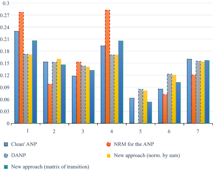

  

  Differences in criteria weights by five methods applied

• In terms of a number of tasks that are done, the lowest number of tasks is related to the situation of DANP and new approaches, and this number is significantly lower than in the first two methods. Since the problem contains only one cluster, there is no difference in the number of tasks between DANP and the new approaches. This difference will exist when the problem is structured through two or more clusters. The DANP calculates priorities in the clusters separately, then priorities between the clusters, and then both priorities are aggregated to final priorities. Therefore, in DANP it is required to identify the intensities of influences between both, elements and clusters. New approach acts like the problem consists of one cluster, even though there are actually two or more clusters. Consequently, only intensities between the elements have to be identified. Hence, the number of tasks in DANP is higher than in the new approach.

• In general, if we have any other problem structure, the situation related to the number of tasks is as follows. Firstly, let us introduce some labels:

  • $m$ = number of clusters.

  • $n_{i}$ = number of criteria in $i$-th cluster.

  • $L_{i}^{j} \left( k \right)$ = number of dependencies between of $i$-th criterion from $j$ cluster considering the element $k$.

  • $l_{i}^{j} \left( k \right)$ = number of the strongest dependencies between of $i$-th criterion from cluster $j$ considering the element $k$ (NRM, DANP).

  Analysis of the number of tasks per each DEMATEL-ANP integration is given in Table 15. Considering the cluster level, we will count each comparison on the cluster level as 5 tasks.

  Table 15 Analysis of the general number of tasks per each DEMATEL-ANP integration

If we sum the columns, then the lowest sum is in the last column.

• Data transformation procedures are related to the number of transformations of original data to obtain the final criteria weights. The goal is to have a method which will use as small as a possible number of original data transformations. There are two reasons for that: one is related to method complexity (lower the number of transformations, lower the complexity of method implementation), and the second is related to credibility of the results (lower the number of transformation, higher the influence of original problem data information on the final results and higher the credibility of the results). In current DEMATEL-ANP approaches, the number of those procedures equals 3: (0) origin input data are identified, (1) input data are transformed to identify the strongest influences and obtain the network structure, (2) local priorities of elements in clusters and local priorities of clusters are calculated and aggregated to weighted supermatrix, (3) weighted supermatrix is transformed to the final criteria weights. In the new approach, the number of those procedures equals 2: (0) origin input data are identified, (1) procedure of sum normalisation or matrix of transition is applied to obtain weighted supermatrix, (2) weighted supermatrix is transformed to the final criteria weights.

• Data loss is related to losing some of the original data in the procedure of calculating the final criteria weights. In NRM for the ANP, the DEMATEL is used to filter the strongest influences between the criteria and further application covers only the strongest influences, not all of them. That means that NRM for the ANP loses some of the original input data. Since all other DEMATEL-ANP integrations include this step of filtering the strongest values, the data loss is present in DANP, too. In the new approach, the DEMATEL is not used to filter the strongest values, and all origin data contribute in the calculation of calculating the final priorities.

• The last criterion is a pairwise comparison (PC). It is related to the characteristic if the DEMATEL-ANP integration keeps the pairwise-comparison procedure somewhere in the calculation. Pairwise comparison is a base of both, AHP and ANP, and if we lose the base, it is questionable if we can still talk about the ANP or not. NRM for the ANP keeps the pair-wise comparison procedure, but only for the strongest influences (dependencies) between the criteria. DANP loses the pairwise comparison procedure completely. In the new approach, in a variant of a matrix of transitions, the pairwise comparison procedure is kept, but it is implemented automatically. Implementation of the automatic pairwise comparisons also contributes to the keeping the consistency at the overall level.

When the input data for four methods’ modifications were collected, the survey participants evaluated the complexity of giving inputs for all methods that they applied and evaluated their understanding of all four methods. A questionnaire based on a Likert scale was used to collect the respondents’ opinions who participated in our workshops. After an analysis of the collected data, we concluded that the newly developed DEMATEL–ANP approach is less complex for decision-makers, but also the most understandable, compared to the other approaches presented in this paper.

The questionnaire contained 4 questions. Participants evaluated the complexity or hardness (mental effort) of implementing 4 activities of giving inputs:

• 1. Determining the existence of influences between the criteria,

• 2. Determining the weights of the influences between the criteria,

• 3. Pairwise comparisons of the criteria with the respect to the goal,

• 4. Pairwise comparisons of the criteria with the respect to the other goals.

After the data were collected, arithmetic means and mods per each activity were calculated. The results are given in Table 16.

Table 16 Analysis of the complexity of giving inputs for DEMATEL-ANP integrations

According to Tables 7 and 16, then the conclusions are the following:

• Since the ‘Clean ANP’ activities 1, 3 and 4; the complexity of the ‘Clean ANP’ is evaluated as 3.45 on average,

• NRM for the ANP covers all activities; the complexity of the NRM for the ANP is 3.21 on average,

• DANP and new approaches cover the activity 2; the complexity is 3.11 on average.

Finally, the duration of the input data collecting was the shortest in case of DANP and new approaches which is logical considering the Table 7.

7 Conclusion

In this paper, we gave an overview of the ANP method with a detailed illustration of its steps that we find crucial, and which are often still not understood by users. Conducting the ANP is a time-consuming activity, and some steps are very challenging. Therefore, the DEMATEL can be used in conjunction with the ANP to decrease the complexity of the ANP method. After presenting the theoretical background of the ANP and the DEMATEL, several DEMATEL–ANP integrations were given, and a new approach was proposed. In a further analysis, the specifics of the approach and the main differences between them were explored. The new approach was demonstrated on a real case and compared with a ‘clean’ ANP and some DEMATEL–ANP integrations in terms of their results, implementation procedures and complexity.

The most important characteristics of the new approach are: (1) the complexity of conducting decision-making is significantly reduced (duration, number of steps [tasks], and the user’s understanding of the method); (2) pairwise comparisons are still a part of the procedure, which became automated; (3) there is no data loss (which occurs, for example, in the NRM for an ANP integration); and finally (4) the number of data transformation procedures is decreased.

Finally, we are finishing with the evaluation the achievements of the goals which are set up in the Sect. 2:

• 1. To present and analyse the characteristics of the ANP and the DEMATEL—presented in Sects. 3 and 4,

• 2. To analyse current integrations of the DEMATEL and the ANP—presented and analysed in Sect. 5.1,

• 3. To develop and present a new DEMATEL–ANP integration approach—presented in Sect. 5.2,

• 4. To demonstrate a new integration approach on a real case example—presented in the Sect. 6.2,

• 5. To analyse a new integration approach and compare it to current integration approaches on a theoretical level—presented in Sect. 6.1,

• 6. To compare the implementation results of a new approach with the implementation results of a ‘clean’ ANP and some of the current DEMATEL–ANP approaches—presented in the Sect. 6.2.

References

Attri R, Dev N, Sharma V (2013) Interpretive structural modelling (ISM) approach: an overview. Res J Manag Sci 2(2):3–8. https://doi.org/10.1108/01443579410062086
Begičević N (2008) Višekriterijski modeli odlučivanja u strateškom planiranju uvođenja e-učenja. University of Zagreb, Faculty of organization and informatics, Doktorski rad
Begicevic Redep N, Klacmer Calopa M, Bockaj J (2015) Decision making on human resource capacity in the higher education institutions. In: ICERI2015 proceedings. IATED, pp 2514–2524
Chang B, Chang CW, Wu CH (2011) Fuzzy DEMATEL method for developing supplier selection criteria. Expert Syst Appl 38(3):1850–1858. https://doi.org/10.1016/j.eswa.2010.07.114
Creswell JW (2014) Research design: qualitative, quantitative, and mixed methods approaches. In: Knight V, Young J, Koscielak K (eds.) Research design qualitative quantitative and mixed methods approaches, 4th edn. SAGE Publications, Inc, Thousand Oaks, California, USA
Divjak B (2017) Webpage od the project development of a methodological framework for strategic decision-making in higher education—a case of open and distance learning (ODL) implementation. Retrieved 7 January 2017, from http://higherdecision.foi.hr/
Gölcük İ, Baykasoğlu A (2016) An analysis of DEMATEL approaches for criteria interaction handling within ANP. Expert Syst App006C 46:346–366. https://doi.org/10.1016/j.eswa.2015.10.041
Hammond J, Keeney R, Raiffa H (1999) Smart choices: a practical guide to making better decisions. Harvard Business School Press, Boston
Harker PT, Vargas LG (1987) The theory of ratio scale estimation: Saaty’s analytic hierarchy process. Manag Sci 33(11):1383–1403. https://doi.org/10.1287/mnsc.33.11.1383
Kadoić N, Begičević Ređep N, Divjak B (2016) E-learning decision making: methods and methodologies. In: Re-imagining learning scenarios, vol Conference. European Distance and E-Learning Network, Budapest, p 24
Kadoić N, Begičević Ređep N, Divjak B (2017a) A new method for strategic decision-making in higher education. Central Eur J Oper Res 1:1. https://doi.org/10.1007/s10100-017-0497-4
Kadoić N, Begičević Ređep N, Divjak B (2017b) Decision making with the analytic network process. In: Kljajić Borštnar M, Zadnik Stirn L, Žerovnik J, Drobne S (eds) SOR 17 proceedings. Slovenia Society Informatika—Section for Operational Research, Bled, Ljubljana, pp 180–186
Kadoić N, Begičević Ređep N, Divjak B (2017c) Structuring e-learning multi-criteria decision making problems. In: Billjanović P (ed) Proceedings of 40th jubilee international convention, MIPRO 2017. Croatian Society for Information and Communication Technology, Electronics and Microelectronics—MIPRO, Opatija, pp 811–817. https://doi.org/10.23919/MIPRO.2017.7973514
Kadoić N, Divjak B, Begičević Ređep N (2017d) Effective strategic decision making on open and distance education issues. In: Volungeviciene A, Szűcs A (eds) Diversity matters!. European Distance and E-Learning Network, Jönköping, pp 224–234
Lee WS, Huang AY, Chang YY, Cheng CM (2011) Analysis of decision making factors for equity investment by DEMATEL and analytic network process. Expert Syst Appl 38(7):8375–8383. https://doi.org/10.1016/j.eswa.2011.01.027
Lin CL, Hsieh MS, Tzeng GH (2010) Evaluating vehicle telematics system by using a novel MCDM techniques with dependence and feedback. Expert Syst Appl 37(10):6723–6736. https://doi.org/10.1016/j.eswa.2010.01.014
Michnik J (2013) Weighted influence non-linear gauge system (WINGS)-An analysis method for the systems of interrelated components. Eur J Oper Res 228(3):536–544. https://doi.org/10.1016/j.ejor.2013.02.007
Ölçer MG (2013) DEMATEL ve ANP Yaklaşımları Kullanılarak Hesap Çizelgelerine Dayalı Bir Karar Destek Sistemi Geliştirilmesi. Fen Bilimleri Enstitüsü 167
Ou Yang YP, Shieh HM, Tzeng GH (2013) A VIKOR technique based on DEMATEL and ANP for information security risk control assessment. Inf Sci 232:482–500. https://doi.org/10.1016/j.ins.2011.09.012
Peffers K, Tuunanen T, Gengler CE, Rossi M, Hui W, Virtanen V, Bragge J (2006) The design science research process: a model for producing and presenting information systems research. In: Proceedings of design research in information systems and technology DESRIST’06, 24, pp 83–106. http://doi.org/10.2753/MIS0742-1222240302
Saaty TL (2001) Decision making with dependence and feedback: the analytic network process: the organization and prioritization of complexity (second and). RWS Publications, New York
Saaty TL (2008) Decision making with the analytic hierarchy process. Int J Serv Sci 1(1):83–98
Saaty TL, Cillo B (2008) A dictionary of complex decision using the analytic network process, the encyclicon, vol 2, 2nd edn. RWS Publications, Pittsburgh
Shao J, Taisch M, Ortega M, Elisa D (2014) Application of the DEMATEL method to identify relations among barriers between green products and consumers. In: 17th European roundtable on sustainable consumption and production—ERSCP 2014, pp 1029–1040. https://core.ac.uk/download/pdf/42968750.pdf. Accessed 15 Dec 2018
Shih-Hsi Y, Wang CC, Teng L-Y, Hsing YM, Yin Shih-Hsi (2012) Application of DEMATEL, ISM, and ANP for key success factor (KSF) complexity analysis in R&D alliance. Sci Res Essays 7(19):1872–1890. https://doi.org/10.5897/SRE11.2252
Springer (n.d.) Spearman rank correlation coefficient. In: The concise encyclopedia of statistics. Springer, New York, pp 502–505. http://doi.org/10.1007/978-0-387-32833-1_379
Sumrit D, Anuntavoranich P (2013) Using DEMATEL method to analyze the causal relations on technological innovation capability evaluation factors in thai technology-based firms. Int Trans J Eng Manag Appl Sci Technol 4(2):81–103
Tsai WH, Chou WC (2009) Selecting management systems for sustainable development in SMEs: a novel hybrid model based on DEMATEL, ANP, and ZOGP. Expert Syst Appl 36(1):1444–1458. https://doi.org/10.1016/j.eswa.2007.11.058
Lu MT, Lin SW (2010) Application of DEMATEL and ANP to investigate strategic drivers for green innovation. The 11th Asia Pacific Industrial Engineering and Management Systems Conference, vol 7, pp 3–8. http://www.apiems.org/archive/apiems2010/pdf/GD/106.pdf
Vaishnavi V, Kuechler B (2004) Design science research in information systems overview of design science research. Ais. https://doi.org/10.1007/978-1-4419-5653-8
Vujanović D, Momčilović V, Bojović N, Papić V (2012) Evaluation of vehicle fleet maintenance management indicators by application of DEMATEL and ANP. Expert Syst Appl 39(12):10552–10563. https://doi.org/10.1016/j.eswa.2012.02.159
Wu WW (2008) Choosing knowledge management strategies by using a combined ANP and DEMATEL approach. Expert Syst Appl 35(3):828–835. https://doi.org/10.1016/j.eswa.2007.07.025
Yang JL, Tzeng GH (2011) An integrated MCDM technique combined with DEMATEL for a novel cluster-weighted with ANP method. Expert Syst Appl 38(3):1417–1424. https://doi.org/10.1016/j.eswa.2010.07.048
Yang Y, Shieh H, Leu J, Tzeng G-H (2008) A novel hybrid MCDM model combined with DEMATEL and ANP with applications. Int J Oper Res 5(3):160–168
Acknowledgements
The work presented in this paper has been supported by the Croatian Science Foundation under the project, ‘Development of a methodological framework for strategic decision-making in higher education—a case of open and distance learning (ODL) implementation’. Project Number: IP-2014-09-7854. Details about the project can be found at the project website, http://higherdecision.foi.hr/en. This paper is a journal version of the paper, ‘Decision-Making with the Analytic Network Process’, which was presented at the SOR 2017 Conference.
Author information
Authors and Affiliations
Corresponding author
Rights and permissions
About this article
Cite this article
Kadoić, N., Divjak, B. & Begičević Ređep, N. Integrating the DEMATEL with the analytic network process for effective decision-making. Cent Eur J Oper Res 27, 653–678 (2019). https://doi.org/10.1007/s10100-018-0601-4
Published:
Issue Date:
DOI: https://doi.org/10.1007/s10100-018-0601-4