
Abstract
Harrington et al. (Math Program Ser B 104:407–435, 2005) introduced a general framework for modeling tacit collusion in which producing firms collectively maximize the Nash bargaining objective function, subject to incentive compatibility constraints. This work extends that collusion model to the setting of a competitive pool-based electricity market operated by an independent system operator. The extension has two features. First, the locationally distinct markets in which firms compete are connected by transmission lines. Capacity limits of the transmission lines, together with the laws of physics that guide the flow of electricity, may alter firms’ strategic behavior. Second, in addition to electricity power producers, other market participants, including system operators and power marketers, play important roles in a competitive electricity market. The new players are included in the model in order to better represent real-world markets, and this inclusion will impact power producers’ strategic behavior as well. The resulting model is a mathematical program with equilibrium constraints (MPEC). Properties of the specific MPEC are discussed and numerical examples illustrating the impacts of transmission congestion in a collusive game are presented.


Notes
The discount factor can be defined as \(\delta := (1-p)/(1+r)\), where \(r\in [0, 1]\) is an interest rate and \(p\in [0, 1]\) represents a probability that the repeated game will end in the next time period.
By definition, the repetition of a static Nash equilibrium is also an SPE. However, not any Nash equilibrium of a repeated game is an SPE.
This is equivalent to the linearized DC representation of power flow, which is an approximation of the actual AC load flow (see Schweppe et al. [41]) and is commonly used in models of electricity markets [45]. In that representation, a hub is arbitrarily chosen, and PTDFs represent the flow on a particular transmission element resulting from a unit injection at the hub and a withdrawal at some other node \(i\). Linearity implies that a transfer of power from a node \(j\) to a node \(i\) can be modeled (and priced) as two transactions: from \(j\) to an arbitrary hub, and then from that hub to \(i\).
Chen et al. [9] have proposed a DC load flow model that considers transmission losses through a (convex) quadratic function. Such an implementation can be incorporated into the modeling and computational approach of the collusion model without much difficulty. As a starting point and for the ease of argument, we omit losses.
Note that since we use an affine function to represent electricity demand at each node, instead of using a fixed demand, there will not be the case that the supply cannot meet the demand.
This is essentially the ISO’s role is, in essence, to eliminate non-congestion related price differentials. Due to this role of the ISO, there cannot be “market sharing” type of agreements (Belleflamme and Bloch [2]) between power producers to preserve their monopoly positions in their “home” markets.
There is another possible type of games (Sauma and Oren [40]) in which the ISO plays as the leader while the oligopolistic power producers act as the follower, with respect to the dispatch schedules. The rationale is that the ISO is aware of the market imperfection, and mitigates the potential market power abuse by strategic generators through anticipating their actions. Under such a setting, the ability that generators may form a tacit collusion is expected to be limited. Such an interesting direction is left to be explored in future research.
Note that the payoffs from a static Nash equilibrium are used as inputs to the collusion model (14) and can be calculated offline. Hence, should there be theoretical and computational advances to address EPEC problems, we can easily substitute the EPEC formulation in calculating the \(\pi _f^N\) for each firm \(f\in \mathcal F \).
However, no proof is known to date for this claim. As a matter of fact, the EPEC game in which each power producer competes while explicitly including in its constraint set all transmission constraints and rivals generation is a generalized Nash equilibrium (GNE) (Yao et al. [47]). Such games are widely recognized to have multiple equilibria (e.g., Oren [34]). A simple example of such a GNE is the pie-sharing game, where each player chooses how much of a pie to take, given how much others have taken; it turns out that if utility is monotonic in the amount of pie, then any split of the pie among the players is an equilibrium. Consequently, there may be some equilibria in the EPEC GNE in which some of the players may be worse-off than playing the CP game.
Note that the variable \(y_f^d\) with an index \(f\) does not mean that it is the deviating firm \(f\)’s decision variable. The index only indicates that it is associated with the ISO’s dispatch decisions when firm \(f\) deviates from the collusive solution.
Note that the complementarity constraints in (18) are from the ISO’s optimization problem, not from the smooth reformulation of the optimal value function of \(\tilde{\pi }^d_f(G_{-f}, a)\).
Though coerciveness of the objective function can guarantee a finite optimal solution without explicit boundedness, (see Proposition A.8 in Bertsekas [4]), the coerciveness of the Nash bargaining objective function cannot be easily shown.
The optimal value functions are written out explicitly through their KKT conditions. The complementarity constraints, with a generic form of \(0\le f(x, y) \perp h(x, y) \ge 0\), are written as \(f(x, y)^Th(x, y)\le 0\). The resulting nonconvex optimization problem sent to BARON (through NEOS server) consists of 40 variables and 67 constraints. The total solving time of this instance is 0.08 s, as BARON finds the optimal solution in preprocessing.
The “Average Price” in Figs. 4 and 5 equals \(\displaystyle \sum \nolimits _{i\in \mathcal N }[p_i\times (\sum \nolimits _{f\in \mathcal F }g_{fi} + y_i)]/ \sum \nolimits _{i\in \mathcal N }\sum \nolimits _{f\in \mathcal F }g_{fi}\).
Fig. 4 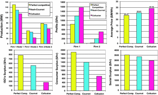
Numerical results under different degrees of market competitiveness
The hub prices under the congested case are 28 $/MWh, 28.26 $/MWh and 28 $/MWh, corresponding to a market of perfect competition, Nash–Cournot and collusion. Without congestion, the nodal prices are the same cross the network, and hence the hub price is the same as the average price reported in Fig. 5.

References
Anderson, E.J., Cau, T.D.H.: Modeling implicit collusion in electricity markets using coevolution. Oper. Res. 57(2), 439–455 (2009)
Belleflamme, P., Bloch, F.: Market sharing agreements and collusive networks. Int. Econ. Rev. 45(2), 387–411 (2004)
Bernheim, B.D., Whinston, M.D.: Multimarket contact and collusive behavior. RAND J. Econ. 21(1), 1–26 (1990)
Bertsekas, D.P.: Nonlinear Programming, 2nd edn. Athena Scientific, Belmont (1999)
Borenstein, S., Bushnell, J., Wolak, F.: Measuring market inefficiencies in California’s wholesale electricity industry. Am. Econ. Rev. 42, 1376–1405 (2002)
Bunn, D.W., Martoccia, M.: Unilateral and collusive market power in the electricity pool of England and Wales. Energy Econ. 27, 305–315 (2005)
Bunn, D.W., Oliveira, F.S.: Agent-based simulation: an application to the new electricity trading arrangements of England and Wales. IEEE Trans. Evolut. Comput. 5(5), 493–503 (2001)
Cardell, J.B., Hitt, C.C., Hogan, W.W.: Market power and strategic interaction in electricity networks. Resour. Energy Econ. 19, 109–137 (1997)
Chen, Y., Hobbs, B.F., Leyffer, S., Munson, T.S.: Leader-follower equilibria for electric power and \(\text{ NO }_x\) allowances markets. Comput. Manag. Sci. 3(4), 307–330 (2006)
Cicchetti, C.J., Dubin, J.A., Long, C.M.: The California Electricity Crisis: What, Why, and What is Next. Springer, Berlin (2004)
Correia, P., Overbye, T., Hiskens, I.: Supergames in electricity markets: beyond the Nash equilibrium concept. In: 14th Power Systems Computation Conference. Sevilla, Spain (2002)
Dirkse, S.P., Ferris, M.C.: A pathsearch damped Newton method for computing general equilibria. Ann. Oper. Res. 68, 211–232 (1996)
Fabra, N.: Tacit collusion in repeated auctions: Uniform versus discriminatory. J. Ind. Econ. 51(3), 271–293 (2003)
Fabra, N., Toro, J.: Price wars and collusion in the Spanish electricity market. Int. J. Ind. Organ. 23(3–4), 155–181 (2005)
Fershtman, C., Pakes, A.: A dynamic oligopoly with collusion and price wars. RAND J. Econ. 31(2), 207–236 (2000)
Fiacco, A.V., Kyparisis, J.: Convexity and concavity properties of the optimal value function in parametric nonlinear programming. J. Optim. Theory Appl. 8, 95–126 (1986)
Friedman, J.W.: A noncooperative equilibrium for supergames. Rev. Econ. Stud. 38, 1–12 (1971)
Friedman, J.W.: Game Theory with Applications to Economics, 2nd edn. Oxford University Press, New York (1990)
Green, E., Porter, R.: Non-cooperative collusion under imperfect price information. Econometrica 52, 87–100 (1984)
Harrington, J.E.: The determination of price and output quotas in a heterogeneous cartel. Int. Econ. Rev. 32, 767–792 (1991)
Harrington, J.E., Hobbs, B.F., Pang, J.S., Liu, A., Roch, G.: Collusive game solutions via optimization. Math. Program. Ser. B 104, 407–435 (2005)
Harvey, S., Hogan, W.: California electricity prices and forward market hedging. Mimeo: John F. Kennedy School of Government, Harvard University (2000)
Hobbs, B.F.: Linear complementarity models of Nash-Cournot competition in bilateral and POOLCO power markets. IEEE Trans. Power Syst. 16(2), 194–202 (2001)
Hobbs, B.F., Metzler, C., Pang, J.S.: Strategic gaming analysis for electric power networks: an MPEC approach. IEEE Trans. Power Syst. 15(2), 638–645 (2000)
Hogan, W.W.: Contract networks for electric power transmission. J. Regul. Econ. 4(3), 211–242 (1992)
Hu, X., Ralph, D.: Using EPECs to model bilevel games in restructured electricity markets with locational prices. Oper. Res. 55(5), 809–827 (2007)
Leyffer, S., Munson, T.: Solving multi-leader-common-follower games. Optim. Methods Softw. 25(4), 601–623 (2010)
Liu, A.L.: Repeated-game models of competitive electricity markets: formulations and algorithms. Ph.D. thesis, Department of Applied Mathematics and Statistics, The Johns Hopkins University, Baltimore, MD (2009)
Liu, A.L.: Repeated games in electricity spot and forward markets—an equilibrium modeling and computational framework. In: 48th Annual Allerton Conference on Communication, Control and Computing, pp. 66–71 (2010)
Macatangay, R.E.A.: Tacit collusion in the frequently repeated multi-unit uniform price auction for wholesale electricity in England and Wales. Eur. J. Law Econ. 13(3), 257–273 (2002)
Metzler, C., Hobbs, B., Pang, J.S.: Nash-Cournot equilibria in power markets on a linearized DC network with arbitrage: formulations and properties. Netw. Spatial Econ. 3(2), 123–150 (2003)
Nash, J.F.: The bargaining problem. Econometrica 18, 155–162 (1950)
Newbury, D.: Regulating unbundled network utilities. Econ. Soc. Rev. 33(1), 23–41 (2002)
Oren, S.S.: Economic inefficiency of passive transmission rights in congested electricity systems with competitive generation. Energy J. 18(1), 63–83 (1997)
Pang, J.S., Fukushima, M.: Quasi-variational inequalities, generalized Nash equilibria, and multi-leader-follower games. Comput. Manag. Sci. 2(1), 21–56 (2005)
Puller, S.L.: Pricing and firm conduct in California’s deregulated electricity market. Rev. Econ. Stat. 89(1), 75–87 (2007)
Rasch, A., Wambach, A.: Internal decision-making rules and collusion. J. Econ. Behav. Organ. 72(2), 703–715 (2009)
Rothkopf, M.H.: Daily repetition: a neglected factor in the analysis of electricity auctions. Electr. J. 12(3), 164–212 (1999)
Sahinidis, N.V., Tawarmalani, M.: BARON 7.2.5: global optimization of mixed-integer nonlinear programs, user’s manual (2005)
Sauma, E.E., Oren, S.S.: Proactive planning and valuation of transmission investments in restructured electricity markets. J. Regul. Econ. 30(3), 261–290 (2006)
Schweppe, F.C., Caramanis, M.C., Tabors, R.D., Bohn, R.E.: Spot Pricing of Electricity. Kluwer Academic, Dordrecht (1988)
Sweeting, A.: Market power in the England and Wales wholesale electricity market 1995–2000. Econ. J. 117, 654–685 (2007)
Tellidou, A.C., Bakirtzis, A.G.: Agent-based analysis of capacity withholding and tacit collusion in electricity markets. IEEE Trans. Power Syst. 22(4), 17–35 (2007)
Twomey, P., Green, R., Neuhoff, K., Newbery, D.: A review of the monitoring of market power. CMI Working Paper 71, University of Cambridge (2005)
Ventosa, M., Baíllo, A., Ramos, A., Rivier, M.: Electricity market modeling trends. Energy Policy 33(7), 897–913 (2005)
Visudhiphan, P., Ilić, M.D.: Dynamic games-based modeling of electricity markets. In: IEEE-PES Annual Conference Proceedings, pp. 274–281. NYC, NY (1999)
Yao, J., Adler, I., Oren, S.: Modeling and computing two-settlement oligopolistic equilibrium in congested electricity networks. Oper. Res. 56(1), 34–47 (2008)
Yao, J., Oren, S.S., Adler, I.: Two-settlement electricity markets with price caps and Cournot generation firms. Eur. J. Oper. Res. 181(3), 1279–1296 (2007)
Acknowledgments
This work is based on the first author’s doctoral dissertation at the Johns Hopkins University, which was advised under Jong-Shi Pang and Benjamin Hobbs. This paper has benefited significantly from collaboration and discussion with Jong-Shi Pang and Joseph Harrington. We also want to thank three anonymous referees and Shmuel Oren (the editor) for their very helpful comments. This research is partially supported by the National Science Foundation (NSF) under the grant ECS-0224817. The second author is also partially supported by NSF under an EFRI Grant 0835879.
Author information
Authors and Affiliations
Corresponding author
Appendices
Appendix 1: Static Nash equilibrium models
1.1 Exogenous-ISO model
For each power producer \(f \in \mathcal F \), again let \(X_f\) denote its generic feasible production region. Then \(f\) solves the following optimization problem.
The ISO solves the following optimization problem.
By writing out the the KKT conditions of each firm’s and the ISO’s optimization problem, together with the market clearing condition, we obtain a complementarity problem (CP).
1.2 Endogenous-ISO model
For each power producer \(f \in \mathcal F \), it solves the following optimization problem.
As each firm’s problem is an MPEC, by grouping all firms’ problems together, we obtain an equilibrium problem with equilibrium constraints (EPECs).
Appendix 2: Algebraic reformulation of the collusion model
This appendix provides the derivation of the model (18) from (17). The key idea is that certain variables in the optimality conditions of the ISO’s optimization problem are redundant. For the ease of argument, we re-provide the optimality conditions in the following.
which is derived under the affine inverse demand function assumption: \( p(d) = P^0 - Bd\).
The purpose of the following derivation is to derive explicit expressions of \(y\) and \(\mu \) with respect to \(G\) and \(\lambda \), hence eliminating the need to keep the (redundant) variables \(y\) and \(\mu \) in the model. Without loss of generality, we assume that node \(N\) is designated as the hub node, and introduce the following notations. Let \(\breve{P}^0, \breve{G}\) and \(\breve{y}\) denote the \(\mathfrak R ^{N-1}\) vectors excluding the \(N\)th component of \(P^0, G\) and \(y\), respectively. Also let \(P_{N}^0, Q_{N}^0\) and \(G_{N}\) denote the \(N\)th component of the vectors \(P^0, Q^0\), and \(G\), respectively. Further use \(\breve{B}\) to denote the \((N-1)\times (N-1)\) matrix resulting from deleting the \(N\)th row and column of \(B\), and \(\breve{\mathbf{1 }}\) to represent an \((N-1)\) vector of 1’s. Notice that by two equations in (26) and (27) we can have the following linear system of \(\mu \) and \(\breve{y}\) with \(G\) and \(\lambda \) as parameters:
where Eq. (29) is the same as in (26) for all the nodes other than the hub node; while Eq. (30) is derived using (26) at the hub node (where \(\mathrm PTDF _{kN}\) for each \(k\in \mathcal A \) is 0) and Eq. (27). Rewriting the linear system (29) and (30) into a matrix form yields the following.
Recall that matrix \(\breve{B} = \mathrm Diag (b_i)\) is an \((N - 1) \times (N - 1)\) diagonal matrix, with \( b_i = P_i^0/Q_i^0,\ i = 1, \ldots , N - 1\). Under the assumption that \(P_i^0 > 0\) and \(Q_i^0 > 0\) for each \(i = 1, \ldots , N,\, \breve{B}\) is positive definite, and so is the skew-symmetric coefficient matrix in (31)
Hence, the coefficient matrix is nonsingular, and the linear system (31) has a unique solution. Let \(H\in \mathfrak R ^{2L \times N}\) denote the \(\mathrm PTDF \) matrix, and \(\breve{H}\in \mathfrak R ^{2L \times (N-1)}\) be the \(H\) matrix with its \(N\)th column removed. Then the solution of (31) can be expressed as follows.
where
With (32) and (33), the three conditions in the ISO’s optimality conditions (26)–(28) can be condensed into one single complementarity constraint:
Let \(r := T - H\breve{R}^0 \in \mathfrak R ^{2L}, \varDelta := -H\breve{\varUpsilon }\in \mathfrak R ^{2L \times N}\) and \(M := H\breve{\varXi }H^T \in \mathfrak R ^{2L\times 2L}\). The above complementarity system can then be written as
Furthermore, with (33) and Eq. (27), each firm’s payoff function \(\pi _f(g_f, y) = p(G + y)^Tg_f - C_f(g_f)\) can be re-written as a function of \((G, \lambda )\) as follows
which is exactly Eq. (19). Hence, we have completed the derivation of (18) from (17).
Proof of Lemma 1
Given the assumptions in Lemma 1, the matrix \(\breve{\varXi }\) is strongly diagonally dominant by the fact that for each \(i = 1, \ldots , N - 1\),
Since \(\breve{\varXi }\) is also symmetric and has positive diagonal entries, it is then a positive definite matrix. Consequently, \(M \!=\! H \breve{\varXi } H^T\) is a symmetric, positive semi-definite matrix.\(\quad \square \)
Rights and permissions
About this article
Cite this article
Liu, A.L., Hobbs, B.F. Tacit collusion games in pool-based electricity markets under transmission constraints. Math. Program. 140, 351–379 (2013). https://doi.org/10.1007/s10107-013-0693-5
Received:
Accepted:
Published:
Issue Date:
DOI: https://doi.org/10.1007/s10107-013-0693-5