
Abstract
We consider the assortment and inventory decisions of a retailer under a locational consumer choice model where products can be differentiated both horizontally (e.g., color of a product) and vertically (e.g., quality of a product). The assortment and quantity decisions affect customer choice and, hence, the demand and sales for each product. In this paper, we investigate two different environments where product availability and assortment affect consumer choice and demand in different ways: make-to-order (MTO) and make-to-stock (MTS). In the MTO environment, customers order and purchase their most preferred product; that is, stockouts do not occur. In the MTS model, customers buy their most preferred product if it is in stock or do not buy if it is out of stock.
In both environments we find conditions under which it is optimal to carry assortments of only a single quality level. In the MTS case, we show that an assortment of mixed quality levels can be optimal only within a narrow range of parameters.


Notes
The existence and uniqueness of \(\underline{d}^{S}_{y}\) follow from the convexity of \(\varPi^{S}_{j}(d_{j}(\mathbf{b},\mathbf{y}))\) and \(\varPi_{j}^{S}(0) = -K < 0\).
References
7thOnline (2007). Inc. Website. Last accessed 11/27/07. http://www.7thonline.com/index.shtm.
Alptekinoğlu, A., & Corbett, C. (2008). Mass customization versus mass production: variety and price competition. Manuf. Serv. Oper. Manag., 10(2), 204–217.
Alptekinoğlu, A., & Corbett, C. (2010). Leadtime-variety tradeoff in product differentiation. Manuf. Serv. Oper. Manag., 12(4), 569–582.
Aydin, G., & Porteus, E. L. (2008). Joint inventory and pricing decisions for an assortment. Operations Research, 56, 1247–1255.
Cachon, G. P., & Kök, A. G. (2007). Category management and coordination in retail assortment planning in the presence of basket shopping consumers. Management Science, 53, 934–951.
Cachon, G. P., Terwiesch, C., & Xu, Y. (2005). Retail assortment planning in the presence of consumer search. Manuf. Serv. Oper. Manag., 7(4), 330–346.
Chen, F., Eliashberg, J., & Zipkin, P. (1998). Consumer preferences, supply chain costs, and product line design. In Ho, Tang (Ed.), Product variety management: research advances, Norwell: Kluwer Academic.
Economides, N. (1989). Quality variations and maximal variety differentiation. Regional Science and Urban Economics, 19, 21–29.
Economides, N. (1993). Quality variations in the circular model of variety-differentiated products. Regional Science and Urban Economics, 23, 235–257.
Heese, S., & Swaminathan, J. (2006). Product line design with component commonality and cost reduction effort. Manufacturing & Service Operations Management, 8(2), 206–220.
Gaur, V., & Honhon, D. (2006). Assortment planning and inventory decisions under a locational choice model. Management Science, 52(10), 1528–1543.
Honhon, D., Gaur, V., & Seshadri, S. (2010). Assortment planning and inventory management under stockout-based substitution. Operations Research, 58(5), 1367–1379.
Hopp, W. J., & Xu, X. (2005). Product line selection and pricing with modularity in design. Manufacturing & Service Operations Management, 7(3), 172–187.
Kök, A. G., & Fisher, M. L. (2007). Demand estimation and assortment optimization under substitution: methodology and application. Operations Research, 55, 1001–1021.
Kök, A. G., Fisher, M. L., & Vaidyanathan, R. (2006). Assortment planning: a review of literature and industry practice. In Retail supply chain management.
Lacourbe, P., Loch, C. H., & Kavadias, S. (2009). Product positioning in a two-dimensional market space. Production and Operations Management, 18(3), 315–332.
Lancaster, K. (1966). A new approach to consumer theory. Journal of Political Economy, 74, 132–157.
Lancaster, K. (1975). Socially optimal product differentiation. The American Economic Review, 65, 567–585.
Marshall, A. W., & Olkin, I. (1979). Inequalities: theory of majorization and its applications. New York: Academic Press
Maddah, B., & Bish, E. K. (2007). Joint pricing, assortment, and inventory decisions for a retailer’s product line. Naval Research Logistics, 54, 315–330.
Mahajan, S., & van Ryzin, G. (2001a). Stocking retail assortments under dynamic consumer substitution. Operations Research, 49(3), 334–351.
Mahajan, S., & van Ryzin, G. (2001b). Inventory competition under dynamic consumer choice. Operations Research, 49(5), 646–657.
Mayorga, M. E. (2006). Essays on Consumer Heterogeneity and Optimal Stochastic Resource Allocation. Dissertation, University of California, Berkeley.
Mayorga, M. E., Kurz, M. E., & McElreath, M. H. (2008). Optimal attributes of mixed quality assortments. In Proceedings of the 2008 industrial engineering research conference, Vancouver, Canada, BC.
McElreath, M. H., Mayorga, M. E., & Kurz, M. E. (2010). Metaheuristics for assortment problems with multiple quality levels. Computers & Operations Research, 37, 1797–1804.
McElreath, M. H., & Mayorga, M. E. (2012). A dynamic programming approach to solving the assortment planning problem with multiple quality levels. Computers & Operations Research, 39, 1521–1529.
Mendelson, H., & Parlakturk, A. (2008). Competitive customization. Manufacturing & Service Operations Management, 10(3), 377–390.
Moorthy, K. S. (1988). Product and price competition in a duopoly. Marketing Science, 7(2), 141–168.
Mussa, M., & Rosen, S. (1978). Monopoly and product quality. Journal of Economic Theory, 18, 301–317.
Netessine, S., & Rudi, N. (2003). Centralized competitive inventory models with demand substitution. Operations Research, 51(2), 329–335.
Porteus, E. L. (2002). Foundations of stochastic inventory theory. Stanford: Stanford Business Books.
Rajaram, K., & Tang, C. S. (1992). The impact of product substitution on retail merchandising. Central European Journal of Operations Research, 135, 582–620.
Smith, S., & Agrawal, N. (2000). Management of multi-item retail inventory systems with demand uncertainty. Operations Research, 48(1), 50–64.
van Ryzin, G., & Mahajan, S. (1999). On the relationship between inventory costst and variety benefits in retail assortments. Management Science, 45(11), 1496–1509.
Acknowledgements
The authors wish to thank the two referees that reviewed this paper and provided valuable comments which led to a much improved manuscript.
Author information
Authors and Affiliations
Corresponding author
Appendices
Appendix A: Proofs for the Make-to-Order (MTO) model
Throughout the appendix, given an assortment (b,y), let Q y (b,y) denote the probability that a randomly selected customer buys a product of quality level y, y∈{H,L}. Note that Q y (b,y) is given by:
In addition, we define two quantities OR j (b,y) and OL j (b,y) which represent, respectively, the overlap between the coverages of products j and j+1 and the overlap between the coverages of products j and j−1. That is,
Note that if OR j (OL j ) is negative, products j and j+1 (j and j−1) are placed sufficiently far apart so that there is no overlap. Hence, if OR j and OL j are non-positive, then the length of product j’s first choice interval, \(b_{j}^{+} - b_{j}^{-}\) equals \(2l_{y_{j}}\). On the other hand, if OR j or OL j is positive, then \(b_{j}^{+} - b_{j}^{-} < 2l_{y_{j}}\).
Consider two assortments, (b,y) and \((\hat {\mathbf{b}},\hat{\mathbf{y}})\). Define
Note from (2) that
Proof of Proposition 1
Properties (i)–(iii) in Proposition 1 can be shown using similar arguments to those used in the proof of Proposition 1 in Gaur and Honhon (2006). Therefore, we focus on Property (iv). If all the products in the optimal assortment are of the same quality, then the result follows immediately from Gaur and Honhon (2006). Thus, it suffices to consider an assortment that has at least one each of high and low quality products and satisfies Proposition 1(i)–(iii). The proof is by contradiction. Suppose an n-product assortment (b,y) is the only optimal assortment and contains a pair of products, i and i+1, such that OR i (b,y)>0 and, hence, \(b_{i}^{+} - b_{i}^{-} < 2l_{y_{i}}\) and \(b_{i+1}^{+} - b_{i+1}^{-} < 2l_{y_{i+1}}\), thereby violating property (iv). We will modify assortment (b,y) by removing the violation of property (iv) and construct an alternate assortment \((\hat{\mathbf{b}}, \hat{\mathbf{y}})\) with the same number of products and \(\mathit{OR}_{i}(\hat{\mathbf{b}}, \hat{\mathbf{y}}) = 0\) which is at least as good as assortment (b,y), yielding a contradiction to the claim that (b,y) is uniquely optimal. We divide the proof into three cases depending on quality types of products i and i+1.
- Case 1 y i =H,y i+1=L or y i =L,y i+1=L::
-
To create new assortment \((\hat{\mathbf{b}},\hat{\mathbf{y}})\), remove product i+1 from assortment (b,y). Let G(b,y) be the gap in coverage left by the removal of product i+1, that is, \(G(\mathbf{b},\mathbf{y})=[(b_{i+2}-l_{y_{i+2}})-(b_{i}+l_{y_{i}})]\). Next, shift products j≥i+2 left by G(b,y) and concatenate product i+1 to the assortment by putting it next to product n. Figure 6 illustrates how we construct assortment \((\hat{\mathbf{b}},\hat{\mathbf{y}})\) from (b,y), and the following equations formalize the relationship between the two assortments.

Fig. 6 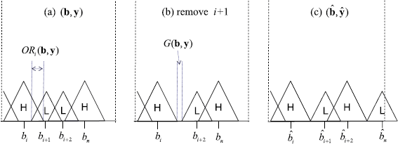
Proposition 1 Case 1, (y i ,y i+1)=(H,L). To construct \((\hat{\mathbf{b}},\hat{\mathbf {y}})\) by modifying (b,y): (a) begin with (b,y); (b) remove i+1, leaving gap G(b,y); (c) shift j≥i+2 left by G(b,y) and concatenate i+1 to end
Notice that the customers who preferred product i+1 in the original assortment (b,y) will now prefer one of the two products that neighbor product i+1 in the original assortment. One or both of these neighboring products may be of high quality. Furthermore, a customer who wished to buy some product in the original assortment (b,y) will continue to do so in the new assortment \((\hat{\mathbf{b}},\hat{\mathbf{y}})\). Therefore, it is not difficult to see that the following two inequalities hold:
 (A.4)
(A.4) (A.5)
(A.5)From (A.1), (A.2), (A.4), and (A.5) we have that
$$\begin{aligned} \varDelta_H&=Q_H(\hat{\mathbf{b}},\hat{ \mathbf{y}})-Q_H(\mathbf{b}, \mathbf{y})\geq Q_L(\hat{ \mathbf{b}}, \hat{\mathbf{y}})-Q_L(\mathbf{b}, \mathbf{y})=- \varDelta_L \end{aligned}$$From the inequality above, (A.3), and the fact that both assortments have the same number of products, we have
$$\varPi^M(\hat{\mathbf{b}}, \hat{\mathbf{y}}) - \varPi^M( \mathbf{b}, \mathbf{y}) = (p_H - c_H) \varDelta_H + (p_L - c_L) \varDelta_L \geq0, $$where the inequality follows from (p H −c H )>(p L −c L ). This concludes the proof of Case 1.
- Case 2 y i =H,y i+1=H::
-
To create a new assortment \((\hat{\mathbf{b}},\hat{\mathbf{y}})\), shift all products j, j≥i+1 right by OR i (b,y) as in Fig. 7. That is,
$$\hat{y}_j=y_j,\quad \forall j; \qquad \hat{b}_j=b_j,\quad i=1,\ldots,i;\qquad \hat{b}_j=b_{j}+\mathit{OR}_i(\mathbf{b},\mathbf{y}), \quad j\geq i+1. $$As in Case 1, we observe that
$$\begin{aligned} & \varDelta_H=Q_H(\hat{\mathbf{b}}, \hat{\mathbf{y}}) -Q_H(\mathbf{b}, \mathbf{y}) \geq0,\quad \mbox{and} \\ & Q_H(\hat{\mathbf{b}}, \hat{\mathbf{y}})+Q_L(\hat{ \mathbf{b}}, \hat{\mathbf{y}}) \geq Q_H(\mathbf{b}, \mathbf{y})+Q_L(\mathbf{b}, \mathbf{y}). \end{aligned}$$From the two inequalities above we again conclude that Δ H ≥−Δ L . This and the assumption that (p H −c H )>(p L −c L ) imply that \(\varPi^{M}(\hat{\mathbf{b}}, \hat{\mathbf{y}}) - \varPi^{M}(\mathbf{b}, \mathbf{y})\geq0\), which concludes the proof of Case 2.
Fig. 7 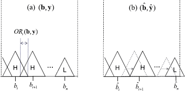
Proposition 1 Case 2: (y i ,y i+1)=(H,H). To construct \((\hat{\mathbf{b}},\hat{\mathbf {y}})\) by modifying (b,y): (a) begin with (b,y); (b) shift all products j≥i+1 right by OR i
- Case 3 y i =L,y i+1=H::
-
This case is a mirror image of the case where y i =H,y i+1=L, which we examined in Case 1. Thus, the result follows from a symmetric argument. □


Proof of Proposition 2
Part (i)
Lemma A.1 in Appendix A shows that the result holds when the quality premium is greater than or equal to the price premium, q≥p H −p L (in other words, l H ≥l L .) Here, we show that the result still holds when l L >l H and condition MH, (p H −c H )l H >(p L −c L )l L , holds. The proof is by contradiction. Suppose an optimal assortment (b,y) contains n products, at least one of which is a low quality product (say product i). We will show that we can always construct an alternate assortment that contains no low quality products and attains higher profits, which yields a contradiction to the optimality of assortment (b,y). To do so, we construct an alternate assortment \((\hat{\mathbf{b}},\hat{\mathbf {y}})\) where \(d_{j}(\mathbf{b}, \mathbf{y})=d_{j}(\hat{\mathbf{b}},\hat{\mathbf{y}})\) for j≠i and product i is replaced by a high quality product.
Now, we consider three cases: 1<i<n,i=1, and i=n.
- Case 1 (1<i<n)::
-
Construct an alternate assortment \((\hat {\mathbf{b}},\hat{\mathbf{y}})\) by replacing low quality product i with a high quality product at the same location (i.e., \(\hat{b}_{i}=b_{i}\)). Note that assortment (b,y) is optimal thus it must satisfy Property (iv) \(b_{i}^{+} - b_{i}^{-} = 2l_{L}\). Furthermore, since 1<i<n, d i (b,y)=2l L . From l H ≤l L , we have \(d_{i}(\hat{\mathbf{b}},\hat{\mathbf{y}})= 2l_{H}\) and \(d_{j}(\mathbf {b}, \mathbf{y})=d_{j}(\hat{\mathbf{b}},\hat{\mathbf{y}})\) for j≠i. Then:
$$\begin{aligned} \varPi^M(\hat{\mathbf{b}}, \hat{\mathbf{y}})- \varPi^M(\mathbf{b}, \mathbf{y})&=\sum_{j=1}^n(p_{\hat{y}_j}-c_{\hat{y}_j})d_j( \hat {\mathbf{b}},\hat{\mathbf{y}})-\sum_{j=1}^n(p_{y_j}-c_{y_j})d_j( \mathbf{b}, \mathbf{y}) \\ &=(p_H-c_H)d_{i}(\hat{\mathbf{b}}, \hat{\mathbf{y}})-(p_L-c_L)d_{i}(\mathbf{b}, \mathbf{y}) \\ &=2 \bigl[(p_H-c_H)l_H-(p_L-c_L)l_L \bigr] > 0, \end{aligned}$$(A.6)where the last inequality follows from Condition MH.
- Case 2 (i=1)::
-
In preparation for the proof, first note that assortment (b,y) is optimal, thus it must satisfy Proposition 1. Hence, \(b_{1}^{+} = b_{1} + l_{L}\) and \(b_{1}^{-} = b_{1} - l_{L}\). It should be noted that it is possible for \(b_{1}^{-}\) to be negative, in which case the first-choice interval for product 1 is \([0, b_{1}^{+}]\). (If that is the case, we say product 1 is truncated.) Now construct an alternate assortment \((\hat{\mathbf{b}},\hat{\mathbf{y}})\) by replacing product 1 of low quality with a high quality product. The locations of all the products remain the same (i.e. \(\hat{b}_{j}=b_{j}\), j≠1) except product 1 whose new location is \(\hat{b}_{1} = b_{1}+(l_{L}-l_{H})\) (so that \(\hat{b}_{1}^{+} =\hat{b}_{1} + l_{H}= b_{1}+l_{L} =b^{+}_{1}\)). This new assortment is shown in Fig. 8. Since \(\hat{b}_{j}=b_{j}\) for j≠1 and \(d_{j}(\mathbf{b}, \mathbf{y})=d_{j}(\hat{\mathbf{b}},\hat{\mathbf{y}})\) for j≠1, we have
$$\begin{aligned} \varPi^M(\hat{\mathbf{b}}, \hat{\mathbf{y}})- \varPi^M(\mathbf{b}, \mathbf{y})&=\sum_{j=1}^n(p_{\hat{y}_j}-c_{\hat{y}_j})d_j( \hat {\mathbf{b}},\hat{\mathbf{y}})-\sum_{j=1}^n(p_{y_j}-c_{y_j})d_j( \mathbf{b}, \mathbf{y}) \\ &=(p_H-c_H)d_{1}( \hat{\mathbf{b}}, \hat{\mathbf{y}})-(p_L-c_L)d_{1}( \mathbf{b}, \mathbf{y}) \end{aligned}$$(A.7)Next observe that \(d_{1}(\hat{\mathbf{b}}, \hat{\mathbf{y}})\) and d 1(b,y) depend on whether or not the products are truncated (whether \(b_{1}^{-} <0\) and/or \(\hat{b}_{1}^{-} <0\)). Since l L >l H , there are only three cases to consider:
-
(i)
If neither product is truncated (\(b_{1}^{-}, \hat{b}^{-}_{1} \geq0\)), then \(d_{1}(\hat{\mathbf{b}}, \hat{\mathbf{y}})=2l_{H}\) and d 1(b,y)=2l L . Hence, \(\varPi^{M}(\hat{\mathbf{b}}, \hat{\mathbf{y}})-\varPi^{M}(\mathbf{b}, \mathbf{y}) > 0\) by condition MH.
-
(ii)
If the low quality product is truncated but the replacement high quality product is not (\(b_{1}^{-}<0\), \(\hat{b}^{-}_{1}\geq 0\)), then \(d_{1}(\hat{\mathbf{b}}, \hat{\mathbf{y}})=2l_{H}\) and d 1(b,y)<2l L , and \(\varPi^{M}(\hat{\mathbf{b}}, \hat{\mathbf{y}})-\varPi^{M}(\mathbf{b}, \mathbf{y}) >0 \) by condition MH.
-
(iii)
If both products are truncated then they achieve the same demand, i.e. \(d_{1}(\hat{\mathbf{b}}, \hat{\mathbf{y}})=d_{1}(\mathbf{b}, \mathbf{y})= b^{+}_{1}\). This combined with (p H −c H )>(p L −c L ) yield \(\varPi^{M}(\hat{\mathbf{b}}, \hat{\mathbf{y}})-\varPi^{M}(\mathbf{b}, \mathbf{y})>0\).
Fig. 8 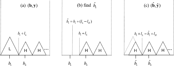
Proposition 2, Case 2, when MH holds and y i =L. To construct \((\hat{\mathbf{b}},\hat{\mathbf{y}})\): (a) begin with (b,y); (b) remove low quality product 1, and find location \(\hat{b}_{1}=b_{1}+(l_{L}-l_{H})\); (c) place a high quality product at location \(\hat{b}_{1}\)
-
(i)
- Case 3 (i=n)::
-
In this case, as in Case 2, we construct an alternate assortment \((\hat{\mathbf{b}},\hat{\mathbf{y}})\) by replacing low quality product n with a high quality product, except that the new location of n is given by \(\hat{b}_{n} = b_{n}-(l_{L}-l_{H})\) (so that \(\hat{b}_{n} - l_{H}= b_{n} - l_{L}\)). We then apply symmetric arguments to show that \(\varPi^{M}(\hat{\mathbf{b}}, \hat{\mathbf{y}})-\varPi ^{M}(\mathbf{b}, \mathbf{y}) >0\).

We have shown that replacing a low quality product with a high quality product improves the profit. Repeating this argument, there exists an optimal assortment consisting of high quality products only.
Part (ii)
If 2(p H −c H )l H <K, then no high quality product is profitable. On the other hand, because K<2(p L −c L )l L , at least one low quality level product is profitable. Thus, when ML holds the optimal assortment will contain only low quality level products. □
Proof of Corollary 2
From Proposition 1 we can write the location of the last product as \(b_{n}=b_{1}+ l_{y_{1}}+\sum_{i=2}^{n-1}2l_{y_{i}}+l_{y_{n}}\), and this satisfies \(\underline{\it{b}}^{M}_{y_{1}}\leq b_{1}< \underline{\it{b}}^{M}_{y_{1}}+2l_{y_{1}}\) and \(\bar{b}^{M}_{y_{n}}-2l_{y_{n}}< b_{n}\leq\bar{b}^{M}_{y_{n}}\). Notice that for the optimal assortment to be of mixed quality types q<p H −p L (equivalently, l L >l H ), otherwise MH holds and the assortment is of high quality types only, therefore l L >l H . Furthermore, since p H >p L we have that \(\underline{b}_{H}^{M} < \underline{b}_{L}^{M}\) and \(\bar{b}_{H}^{M} > \bar{b}_{L}^{M}\).
To calculate the upper bound, we see that \(\bar{b}_{H}^{M}\geq b_{n}\geq (n-1)2l_{H} + b_{1}\geq(n-1)2l_{H} + \underline{b}_{H}^{M}\). This implies that \(n\leq\frac{\bar{b}^{M}_{H}-\underline{b}^{M}_{H}}{2l_{H}} +1\). For the lower bound we see that \(\bar{b}_{L}^{M}-2l_{L}\leq b_{n}\leq(n-1) 2l_{L} + b_{1}\leq(n-1)2l_{L} + \underline{b}_{L}^{M}+2l_{L}=n2l_{L}+ \underline{b}_{L}^{M}\). This implies that \(n\geq \frac{\bar{b}^{M}_{L}-\underline{b}^{M}_{L}}{2l_{L}}-1\). Since n is integer it follows that
□
Lemma A.1
If q≥p H −p L , then the optimal assortment consists of only high quality products.
Proof
The proof is by contradiction. Suppose q≥p H −p L (equivalently, l H ≥l L ) but an optimal assortment (b,y) contains at least one low quality product. We will show that we can always construct an alternate assortment that contains no low quality products and attains higher profits, which yields a contradiction to the optimality of assortment (b,y). Therefore the optimal assortment consists only of high quality products.
Let product i be a low quality product in optimal assortment (b,y). We construct an alternate assortment \((\hat{\mathbf{b}},\hat{\mathbf{y}})\) by replacing low quality product i with a high quality product at the same location b i . (An illustration of this is provided in Fig. 9.) That is,
By assumption, l H ≥l L ; and by construction, locations \(\hat{b}_{j}=b_{j}\) for all j. Therefore \(\hat{b}_{i}^{+}> b_{i}^{+}\) and \(\hat{b}_{i}^{-}<b_{i}^{-}\). Observe that, all customers who preferred low quality product i in the original assortment (b,y) will now prefer the high quality product that replaced it in \((\hat{\mathbf{b}},\hat {\mathbf{y}})\). Therefore, Δ H >0. In addition, a customer who wished to buy some product in assortment (b,y), will continue to do so in assortment \((\hat{\mathbf{b}},\hat{\mathbf{y}})\), thus \(Q_{H}(\hat{\mathbf{b}},\hat{\mathbf{y}})+Q_{L}(\hat{\mathbf {b}},\hat{\mathbf{y}})\geq Q_{H}(\mathbf{b},\mathbf{y})+Q_{L}(\mathbf {b},\mathbf{y})\). These last two observations together imply that Δ H ≥−Δ L . Using this observation, (A.3), and the fact that (p H −c H )>(p L −c L ), we conclude that assortment \((\hat{\mathbf{b}}, \hat{\mathbf{y}})\) is better than assortment (b,y), i.e., \(\varPi^{M}(\hat{\mathbf{b}}, \hat{\mathbf{y}})- \varPi^{M}(\mathbf{b}, \mathbf{y})>0\).

Lemma A.1—To construct \((\hat {\mathbf{b}},\hat{\mathbf{y}})\): (a) begin with (b,y), (b) replace product i with a high quality product at location b i
To complete the proof, we repeat this argument until we remove all low quality products. □
Appendix B: Proofs for the Make-to-Stock (MTS) model
The proofs in this section will use the following definitions.
Definition B.1
(Marshall and Olkin 1979)
For any real vector x=(x 1,x 2,…,x n )∈ℜn, let x [1]≥x [2]⋯≥x [n] denote the components of x in non-increasing order.
- B1.1 :
-
For x,y∈ℜn, we say x is majorized by y, written as x≺y, if
$$\begin{aligned} \sum_{i=1}^kx_{[i]}\leq\sum _{i=1}^k y_{[i]},\quad k=1,\ldots,n-1 \quad \mbox{and}\quad \sum_{i=1}^nx_{[i]}= \sum_{i=1}^ny_{[i]}. \end{aligned}$$(B.1) - B1.2 :
-
x≺y if and only if ∑g(x i )≤∑g(y i ) for all continuous convex functions g:ℜ→ℜ
We carry the following notation from Appendix A: \(Q_{y}(\mathbf{b},\mathbf{y})=\sum_{j:y_{j}=y}d_{j}(\mathbf{b},\mathbf {y})\mbox{ for }y\in\{L,H\}\), \(\mathit{OR}_{j}(\mathbf{b},\mathbf{y})=(b_{j} + l_{y_{j}}) - (b_{j+1}-l_{y_{j+1}})\), and \(\mathit{OL}_{j}(\mathbf{b},\mathbf{y})=(b_{j-1}+l_{y_{j-1}}) - (b_{j}-l_{y_{j}})\).
In addition, define two real functions g H and g L (on the domain of [0,1]) which represent the induced profit for high and low quality products with the first choice probability d excluding the fixed cost K, respectively:
Lastly, define d(b,y)=(d 1(b,y),…,d n (b,y)), which is a vector containing the first choice probabilities of every product in the assortment. Similarly, define \(\mathbf{d}^{y}(\mathbf{b},\mathbf{y})=(d_{1}(\mathbf{b},\mathbf {y})1_{\{y_{1}=y\}},\ldots,d_{n}(\mathbf{b},\mathbf{y})1_{\{y_{n}=y\}}) =(d_{1}^{y},\ldots,d_{n}^{y})\), for y∈{L,H} as the vector containing the first choice probabilities of products of quality level y in the assortment. That is, d y(b,y) is a vector of components \(d_{i}^{y}(\mathbf{b},\mathbf{y})=d_{i}(\mathbf {b},\mathbf{y})1_{\{y_{i}=y\}}\), where \(d_{i}^{y}(\mathbf{b},\mathbf{y})\) is equal to d i (b,y) if y i =y and 0 otherwise. Using this notation and (6), we can rewrite the profit function as
Proof of Proposition 3
The first three properties in Proposition 1 can be shown following similar arguments used in the proof of Proposition 1 in Gaur and Honhon (2006). Thus, we only focus on the last property, Property (iv). If all the products in the optimal assortment are of the same quality, then the result follows immediately from Gaur and Honhon (2006). Thus, it suffices to consider an assortment that has at least one each of high and low quality products and satisfies Proposition 3(i)–(iii).
The proof is by contradiction. Suppose (b,y) is the unique optimal assortment and contains at least one pair of products, i and i+1 that do not satisfy property (iv), i.e. \(b_{i}^{+} - b_{i}^{-} < 2l_{y_{i}}\), and \(b_{i+1}^{+} - b_{i+1}^{-} < 2l_{y_{i+1}}\). We construct an alternate assortment \((\hat{\mathbf{b}}, \hat{\mathbf{y}})\) which satisfies Property (iv) (i.e., \(b_{j}^{+}-b_{j}^{-}=2l_{y_{j}}\) for all j) and is at least as good as assortment (b,y). This leads to a contradiction to (b,y) being uniquely optimal. Let n L and n H be the numbers of low and high quality products in assortment (b,y), respectively. Thus, the total number of products is n=n L +n H .
Define β=Q L (b,y) and γ=Q H (b,y). Note that β+γ≤1. We construct a new assortment \((\hat{\mathbf{b}},\hat{\mathbf {y}})\) by placing all high quality products to the right of 1−γ and all low quality products to the left of β and stretching products to remove any overlap, i.e., \(\hat{b}^{+}_{j}-\hat{b}^{-}_{j}=2l_{\hat{y}_{j}}\) for all j. That is
An illustrative example of \((\hat{\mathbf{b}},\hat{\mathbf{y}})\) is shown in Fig. 10.

Proposition 3, case when \(b_{i}^{+}-b_{i}^{-}<2l_{y_{i}}\) for some i. To create \((\hat{\mathbf {b}},\hat{\mathbf{y}})\): (a) begin with (b,y) and find β and γ; (b) place all high quality products right of 1−γ, and all low quality products left of β; (c) move products to remove any overlaps, i.e. such that \(\hat{b}^{+}_{j}-\hat{b}^{-}_{j}=2l_{y_{j}}\) for all j
By construction, assortment \((\hat{\mathbf{b}},\hat{\mathbf{y}})\) satisfies Property (iv) with low quality products indexed 1 through n L , and high quality products indexed n L +1 to n. Thus we can write
Define two vectors
Now, from (B.3), we observe that there exists k∈{1,…,n L } such that
Again, from (B.4), we observe that there exists k∈{1,…,n H } such that
On the other hand, the demand vectors of high quality products and low quality products in the original assortment (b,y) are
Note that
and
Since \(d^{L}_{[j]}(\mathbf{b},\mathbf{y})\leq2l_{L} \mbox{ for } j=1,\ldots, n_{L}\), from (B.5) and (B.7)
Similarly, since \(d^{H}_{[j]}(\mathbf{b},\mathbf{y})\leq2l_{H} \mbox{ for } j=1,\ldots, n_{H}\), from (B.6) and (B.8)
From Lemma B.1, g y(d), y∈{H,L} is convex in d≥0. Hence,
where the last inequality follows from the definition of majorization and (B.9) and (B.10). □
Proof of Proposition 4
Part (i)
Lemma B.3 in Appendix B shows that the result holds when q≥p H −p L (equivalently, l H ≥l L .) Here, we show that the result still holds when l L >l H and condition SH, g H(2l H )>g L(2l L ), holds. Furthermore, it suffices to consider the case where 2l L <1 because the case with 2l L ≥1 follows trivially from condition SH.
The proof is by contradiction. Suppose an optimal assortment (b,y) contains n products, at least one of which is a low quality product (say product i). We will show that we can always construct an alternate assortment that contains no low quality products and attains higher profits, which yields a contradiction to the optimality of assortment (b,y). To do so, we construct an alternate assortment \((\hat{\mathbf{b}},\hat{\mathbf {y}})\) where \(d_{j}(\mathbf{b}, \mathbf{y})=d_{j}(\hat{\mathbf{b}},\hat{\mathbf{y}})\) for j≠i and product i is replaced by a high quality product.
Now, consider three cases:
- Case 1 (1<i<n)::
-
Construct an alternate assortment \((\hat {\mathbf{b}},\hat{\mathbf{y}})\) by replacing low quality product i with a high quality product at the same location (i.e., \(\hat{b}_{i}=b_{i}\)). Note that assortment (b,y) is optimal thus it must satisfy Property (iv) \(b_{i}^{+} - b_{i}^{-} = 2l_{L}\). Furthermore, since 1<i<n, d i (b,y)=2l L . From l H ≤l L , we have \(d_{i}(\hat{\mathbf{b}},\hat{\mathbf{y}})= 2l_{H}\) and \(d_{j}(\mathbf {b}, \mathbf{y})=d_{j}(\hat{\mathbf{b}},\hat{\mathbf{y}})\) for j≠i. Then:
$$\begin{aligned} \varPi^S(\hat{\mathbf{b}}, \hat{\mathbf{y}})-\varPi^S( \mathbf{b}, \mathbf{y})= \varPi^S_i (\hat{\mathbf{b}}, \hat{\mathbf{y}})- \varPi^S_i (\mathbf{b}, \mathbf{y})=g^H(2l_H) - g^L(2l_L) >0 \end{aligned}$$from condition SH.
- Case 2 (i=1)::
-
In preparation for the proof, first note that assortment (b,y) is optimal, thus it must satisfy Proposition 1. Hence, \(b_{1}^{+} = b_{1} + l_{L}\) and \(b_{1}^{-} = b_{1} - l_{L}\). It should be noted that it is possible for \(b_{1}^{-}\) to be negative, in which case the first-choice interval for product 1 is \([0, b_{1}^{+}]\). (If that is the case, we say product 1 is truncated.) Now construct an alternate assortment \((\hat{\mathbf{b}},\hat{\mathbf{y}})\) by replacing product 1 of low quality with a high quality product. The locations of all the products remain the same (i.e. \(\hat{b}_{j}=b_{j}\), j≠1) except product 1 whose new location is \(\hat{b}_{1} = b_{1}+(l_{L}-l_{H})\) (so that \(\hat{b}_{1}^{+} =\hat{b}_{1} + l_{H}= b_{1}+l_{L} =b^{+}_{1}\)). Since \(\hat{b}_{j}=b_{j}\) for j≠1 and \(d_{j}(\mathbf{b}, \mathbf{y})=d_{j}(\hat{\mathbf{b}},\hat{\mathbf{y}})\) for j≠1, we have
$$\begin{aligned} \varPi^S(\hat{\mathbf{b}}, \hat{\mathbf{y}})-\varPi^S( \mathbf {b}, \mathbf{y}) =\varPi^S_i (\hat{\mathbf{b}}, \hat{\mathbf{y}})- \varPi^S_i (\mathbf{b}, \mathbf{y})=g^H\bigl(d_1 (\hat{\mathbf{b}},\hat{\mathbf {y}})\bigr) - g^L\bigl(d_1 (\mathbf{b},\mathbf{y})\bigr) \end{aligned}$$(B.11)Next observe that \(d_{1}(\hat{\mathbf{b}}, \hat{\mathbf{y}})\) and d 1(b,y) depend on whether or not the products are truncated (whether \(b_{1}^{-} <0\) and/or \(\hat{b}_{1}^{-} <0\)). Since l L >l H , there are only three cases to consider:
-
(i)
If neither product is truncated (\(b_{1}^{-}, \hat{b}^{-}_{1} \geq0\)), then \(d_{1}(\hat{\mathbf{b}}, \hat{\mathbf{y}})=2l_{H}\) and d 1(b,y)=2l L . Hence, \(\varPi^{S}(\hat{\mathbf{b}}, \hat{\mathbf{y}})-\varPi^{S}(\mathbf{b}, \mathbf{y}) =g^{H}(2 l_{H}) - g^{L}(2 l_{L}) >0\) by condition SH.
-
(ii)
If the low quality product is truncated but the replacement high quality product is not (\(b_{1}^{-}<0\), \(\hat{b}^{-}_{1}\geq 0\)), then \(d_{1}(\hat{\mathbf{b}}, \hat{\mathbf{y}})=2l_{H}\) and d 1(b,y)<2l L . Then,
$$\varPi^S(\hat{\mathbf{b}}, \hat{\mathbf{y}})-\varPi^S( \mathbf{b}, \mathbf{y}) =g^H(2 l_H) - g^L \bigl(d_1 (\mathbf{b},\mathbf{y})\bigr) \geq g^H(2 l_H) - g^L(2 l_L) > 0. $$The first inequality holds because g L(d) is increasing in d from Lemma B.2 and \(d_{1} (\mathbf{b},\mathbf{y})\geq\underline {d}^{S}_{L}\) (otherwise, g L(d 1(b,y))<K so product 1 generates loss and would not be a part of the optimal assortment). The second inequality comes from condition SH.
-
(iii)
If both products are truncated then they achieve the same demand, i.e. \(d_{1}(\hat{\mathbf{b}}, \hat{\mathbf{y}})=d_{1}(\mathbf{b}, \mathbf{y})= b^{+}_{1}\). Then
$$\varPi^S(\hat{\mathbf{b}}, \hat{\mathbf{y}})-\varPi^S( \mathbf{b}, \mathbf{y}) =g^H\bigl(b_1^+\bigr) - g^L\bigl(b_1^+\bigr) >0 \quad\mbox{by Lemma B.2}. $$
-
(i)
- Case 3 (i=n)::
-
In this case, as in Case 2, we construct an alternate assortment \((\hat{\mathbf{b}},\hat{\mathbf{y}})\) by replacing low quality product n with a high quality product, except that the new location of n is given by \(\hat{b}_{n} = b_{n}-(l_{L}-l_{H})\) (so that \(\hat{b}_{n} - l_{H}= b_{n} - l_{L}\)). We then apply symmetric arguments to show that \(\varPi^{S}(\hat{\mathbf{b}}, \hat{\mathbf{y}})-\varPi ^{S}(\mathbf{b}, \mathbf{y}) >0\).
We have shown that replacing a low quality product with a high quality product improves the profit. Repeating this argument, there exists an optimal assortment consisting of high quality products only.
Part (ii)
Omitted since proof is similar to that of Proposition 2 Part (ii). □
Proof of Corollary 4
Part (i)
For an assortment consisting of a single quality level y, apply Corollary 1 of Gaur and Honhon (2006), replacing β with \(\bar{b}^{S}_{y}\) and L with l y .
Part (ii)
We omit this proof since it is similar to the proof of Corollary 2. □
Proof of Proposition 5
Clearly \((p_{H}-c_{H})\lambda2l_{H}\geq(p_{H}-c_{H})\lambda 2l_{H}-p_{H}\phi(z_{H})\sqrt{\lambda2l_{H}}\). Thus, if K≥(p H −c H )λ2l H , then \(K\geq(p_{H}-c_{H})\lambda 2l_{H}-p_{H}\phi(z_{H})\sqrt{\lambda2l_{H}}\), and the result follows. □
Proof of Proposition 6
For both cases (MTO and MTS), it is not hard to show that b 1=l y . Applying Corollary 1 to \(n^{*}_{M}(y)\) and Corollary 4(i) to \(n_{S}^{*}(y)\), we have
Since \(\underline{d}^{S}_{y} \geq\underline{d}^{M}_{y}\), we have \(\bar{b}^{S}_{y} \leq\bar{b}^{M}_{y}\), which implies that \(n^{*}_{S}(y)\leq n^{*}_{M}(y)\). To show that \(n^{*}_{M}(y)\) is bounded above, notice that \(\bar{b}^{S}_{y} \geq1- l_{y}\) (since it is profitable to place a product at 1−l y ) and that \(\bar{b}^{M}_{y} \leq1+ l_{y}\)(otherwise, there is no demand). Therefore,
□
Technical lemmas used in Appendix B
Lemma B.1
g y(d),y∈{L,H}, is convex in d≥0. Furthermore, it is increasing in \(d \geq\underline{d}^{S}_{y}\).
Proof
Differentiating g y(d) with respect to d we obtain, \([g^{y}(d)]'=\lambda(p_{y}-c_{y})-\tfrac{p_{y}\phi(z_{y})\lambda }{2\sqrt{\lambda d}}\). Then, the second derivative is \([g^{y}(d)]''=\frac{p_{y}\phi(z_{y})\lambda^{2}}{4(\lambda d)^{\frac{3}{2}}}\). Notice that [g y(d)]″≥0 for d≥0. Thus, the function g y(d) is convex in d for all d≥0. Now, note that g y(d)=0 for d=0. Furthermore, by definition of \(\underline{d}^{S}_{y}\), g y(d)=K for \(d = \underline{d}^{S}_{y}\). Given that g y(d) is convex, there must exist some \(d_{0} \in[0, \underline{d}^{S}_{y}]\) such that g y(d) is increasing in d for all d≥d 0. □
Lemma B.2
g H(d)>g L(d) for any d>0.
Proof
By definition, g y(d)=max x {p y E[min(x,D)]−c y x}, where D is normally distributed with mean λd and standard deviation \(\sqrt{\lambda d}\). Let \(x^{*}_{H}=\arg\max_{x}\{p_{H}E[\min(x,D)] -c_{H}x\}\) and \(x^{*}_{L}=\arg\max_{x}\{p_{L}E[\min(x,D)] -c_{L}x\}\). To see this note that,
Therefore \(\frac{g^{H}(d)}{g^{L}(d)}>\frac{c_{H}}{c_{L}} \geq1\), which implies that g H(d)>g L(d). □
Lemma B.3
If the quality premium is greater than or equal to the price premium, q≥p H −p L , (equivalently l H ≥l L ), then the optimal assortment consists of only high quality products.
Proof
The proof is by contradiction. Suppose (b,y) is an optimal assortment containing at least one low quality product. We show that there exists an alternate assortment with no low quality products which is at least as good as assortment (b,y).
Let product i be the first low quality product in (b,y), i.e. i=min{j:y j =L}. We divide the proof into two cases: i=1 or n, and 1<i<n.
- Case 1: i=1 or i=n.:
-
For i=1, we construct an alternate assortment \((\hat{\mathbf{b}},\hat{\mathbf {y}})\) with y 1=H and \(\hat{b}_{1}^{+}=b_{1}^{+}\). All other products (j≥2) remain unchanged, that is, \((\hat{b}_{j},\hat{y}_{j})=(b_{j},y_{j})\) for all j≥2. Thus, \(d_{j}(\hat{\mathbf{b}},\hat{\mathbf {y}})=d_{j}(\mathbf{b},\mathbf{y})\) for all j≥2. Hence \(\varPi_{j}^{S}(\hat{\mathbf{b}},\hat{\mathbf{y}})= \varPi ^{S}_{j}(\mathbf{b},\mathbf{y})\) for j≥2.
Since l H ≥l L , we have that \(d_{1}(\hat{\mathbf{b}},\hat {\mathbf{y}})\geq d_{1}(\mathbf{b},\mathbf{y})\). Now, from Lemma B.1, we have \(\varPi_{1}^{S}(d_{1}(\hat{\mathbf{b}},\hat{\mathbf{y}}))=g^{H}(d_{1}(\hat {\mathbf{b}},\hat{\mathbf{y}})) - K \geq g^{H}(d_{1}(\mathbf{b},\mathbf {y})) - K\). Furthermore, from Lemma B.2, we have \(g^{H}(d_{1}(\mathbf{b},\mathbf{y})) - K \geq g^{L}(d_{1}(\mathbf{b},\mathbf {y})) - K=\varPi^{S}_{1}(d_{1}(\mathbf{b},\mathbf{y}))\). These last two observations together yield \(\varPi_{1}^{S}(d_{1}(\hat{\mathbf {b}},\hat{\mathbf{y}})) \geq \varPi^{S}_{1}(d_{1}(\mathbf{b},\mathbf{y}))\). Thus, \(\varPi^{S}(\hat {\mathbf{b}},\hat{\mathbf{y}})\geq\varPi^{S} (\mathbf{b},\mathbf{y})\).
For i=n, symmetric arguments apply, so we omit the proof.
- Case 2: i∈{2,…,n−1}.:
-
Construct an alternate assortment \((\hat{\mathbf{b}},\hat{\mathbf{y}})\) by replacing product i with a high quality product at location \(\hat{b}_{i} = b_{i} - (l_{H} -l_{L})\) and shifting the locations of products 1 through i−1 to the left by l H −l L . The new assortment is illustrated in Fig. 11, and the following equations formalize the relationship between assortments (b,y) and \((\hat{\mathbf{b}},\hat {\mathbf{y}})\).

Since the profits from product i+1 to product n are identical in both assortments, (b,y) and \((\hat{\mathbf {b}},\hat{\mathbf{y}})\), we restrict our attention to the profit generated by first i products in the assortment.
Fig. 11 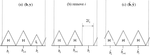
Lemma B.3, Case 2, i=min{j:y j =L}. To create \((\hat{\mathbf{b}},\hat{\mathbf{y}})\): (a) begin with (b,y); (b) remove product i leaving a gap of 2l L ; (c) shift all products j≤i−1 left by l H −l L and replace product i with a high quality product at location \(\hat{b}_{i}=b_{i}-(l_{H}-l_{L})\)
We now consider two cases:
-
(i)
\((b_{i}^{+} \geq2(i-1)l_{H} + 2l_{L} )\): In assortment (b,y), d j (b,y)=2l H for j=1,…,i−1 and d i (b,y)=2l L . In the new assortment \((\hat{\mathbf{b}},\hat{\mathbf{y}})\), we will have \(d_{j} (\hat{\mathbf{b}},\hat{\mathbf{y}})= 2l_{H}\) for j=2,…,i and \(d_{1}(\hat{\mathbf{b}},\hat{\mathbf{y}})\) will be at least as large as 2l L . Hence:
$$\begin{aligned} \varPi^S (\hat{\mathbf{b}},\hat{\mathbf{y}})- \varPi^S ( \mathbf {b},\mathbf{y})&= g^H\bigl(d_1 (\hat{\mathbf{b}}, \hat{\mathbf{y}})\bigr) - g^L(2l_L) \\ &\geq g^H(2l_L) - g^L(2l_L) > 0 \end{aligned}$$The first inequality follows from Lemma B.1, since \(d_{1} (\hat{\mathbf{b}},\hat{\mathbf{y}})\geq2 l_{L} \geq \underline{d}_{L}^{S} \geq \underline{d}_{H}^{S}\). The second inequality follows from Lemma B.2.
-
(ii)
\((b_{i}^{+} < 2(i-1)l_{H} + 2l_{L} )\): First, notice that \(\sum_{j=1}^{n} d_{j} (\mathbf{b},\mathbf{y})= \sum_{j=1}^{n} d_{j}((\hat{\mathbf {b}},\hat{\mathbf{y}})) = b_{i}^{+}\), that is, all customers located between 0 and \(b_{i}^{+}\) will be covered in both assortments (b,y) and \((\hat{\mathbf{b}},\hat{\mathbf {y}})\). Furthermore, in the new assortment \((\hat{\mathbf{b}},\hat {\mathbf{y}})\), we have either \(d_{j} (\hat{\mathbf{b}},\hat{\mathbf{y}})= 2 l_{H}\) for j=2,…,i and \(d_{1} (\hat{\mathbf{b}},\hat{\mathbf{y}})= b_{i}^{+} - 2 (i-1) l_{H}\) or \(d_{j} (\hat{\mathbf{b}},\hat{\mathbf{y}})= 2 l_{H}\) for j=3,…,i, \(d_{2} (\hat{\mathbf{b}},\hat{\mathbf{y}})= b_{i}^{+} - 2 (i-2) l_{H}\) and \(d_{1} (\hat{\mathbf{b}},\hat{\mathbf{y}})=0\). In either case, the demand vector \((d_{1}(\hat{\mathbf{b}},\hat {\mathbf{y}}), \ldots, d_{i}(\hat{\mathbf{b}},\hat{\mathbf{y}}))\) majorizes any other vector (x 1,…,x i ) such that \(\sum_{j=1}^{i} x_{j} = b_{i}^{+}\) and 0≤x j ≤2l H . Therefore:
$$\begin{aligned} \varPi^S (\hat{\mathbf{b}},\hat{\mathbf{y}})- \varPi^S ( \mathbf {b},\mathbf{y})&= \sum_{j=1}^i g^H\bigl(d_j (\hat{\mathbf{b}},\hat {\mathbf{y}})\bigr) - \sum_{j=1}^{i-1} g^H \bigl(d_j (\mathbf{b},\mathbf{y})\bigr) - g^L(2 l_L) \\ &> \sum_{j=1}^i g^H \bigl(d_j (\hat{\mathbf{b}},\hat{\mathbf{y}})\bigr) - \sum _{j=1}^{i} g^H\bigl(d_j ( \mathbf{b},\mathbf{y})\bigr) \geq0 \end{aligned}$$where the first inequality follows from Lemma B.2 and the last inequality follows from \((d_{1}(\hat{\mathbf {b}},\hat{\mathbf{y}}), \ldots, d_{i}(\hat{\mathbf{b}},\hat{\mathbf{y}})) \succ(d_{1}(\mathbf {b},\mathbf{y}), \ldots, d_{i}(\mathbf{b},\mathbf{y}))\). □
-
(i)


Rights and permissions
About this article
Cite this article
Mayorga, M.E., Ahn, HS. & Aydin, G. Assortment and inventory decisions with multiple quality levels. Ann Oper Res 211, 301–331 (2013). https://doi.org/10.1007/s10479-013-1456-7
Published:
Issue Date:
DOI: https://doi.org/10.1007/s10479-013-1456-7