A New Steepest Descent Differential Inclusion-Based Method for Solving General Nonsmooth Convex Optimization Problems

Abstract

In this paper, we investigate a steepest descent neural network for solving general nonsmooth convex optimization problems. The convergence to optimal solution set is analytically proved. We apply the method to some numerical tests which confirm the effectiveness of the theoretical results and the performance of the proposed neural network.

1 Introduction

Nonsmooth optimization problems belong to important categories of applied problems in industry, engineering, and economics. Different methods have been introduced for solving such problems since the 1960s. Nonsmooth optimization problems are important because of their scientific and engineering applications (see [1–3] and references therein). These problems are difficult to solve, even in the unconstrained cases. Some algorithms for solving such problems are available, such as subgradient methods [4], cutting plane methods [5], analytic center cutting plane methods [6], bundle methods [7–9], and differential inclusion-based methods [10–13]. Most of these methods are feasible in the sense that, for solving a constrained optimization problem, the initial condition must be chosen from inside of the feasible region; for more details see, for example, [14] and [15]. On the other hand, some versions of bundle methods (see, for example, [16, 17]) as well as some differential inclusion-based methods, such as the methods of [10, 11] and the one proposed by us, can deal with infeasible starting points. In these methods, it is possible to choose the initial condition from outside of the feasible region while still being convergent. This fact is one of the most important features which differentiates these methods from some other conventional ones. It is also a reason for authors to try to develop methods of this class for solving optimization problems. From differential equation-based and differential inclusion-based methods for solving optimization problems, we can refer to four different classes: gradient projection methods [12, 13, 18, 19], primal–dual methods [20, 21], Lagrange multiplier rule methods [22], penalty-based methods [10, 11], or some combination of these methods. Gradient projection-based methods are among those which have received a lot of attention in recent years. In these methods, the right-hand side of the designed differential inclusion is a projection of a subgradient function (which is dependent on the objective function) on the feasible solution set. While finding projections on simple sets in ℝⁿ (e.g., those given by box constraints) is an easy task, it is more challenging on complex sets. Although primal–dual methods are efficient for solving some special problems, like quadratic programming problems, they are not efficient for solving more general optimization problems. Lagrange multiplier methods have been designed for problems with nonsmooth objective functions with special constraints, e.g., linear ones. Among them, the penalty-based methods are the most robust ones. One of the basic methods for a general form of convex optimization problem is the neural network introduced by Forti et al., which is a penalty-based method. This method has several valuable properties: first, its global convergence is guaranteed. Second, the initial condition can be selected from outside of the feasible region. And, third, the convergence to feasible region in finite time is established. On the contrary, the selection of an appropriate penalty parameter can be considered a limitation concern of this method, as the convergence is guaranteed for a sufficiently large penalty parameter. Furthermore, the performance of the method for different values of penalty parameters cannot be anticipated beforehand; for example, bigger values do not guarantee better performance. However, in this paper, we will introduce a penalty parameter free, new neural network for solving general nonsmooth convex optimization problems based on a different analytical formulation. In this neural network, the calculation of projections is not required and there is no need to increase the dimension of the problem.

The rest of the paper is organized as follows. In Sect. 2, we formulate the problem and describe some concepts that are used in the rest of the paper. In Sect. 3, first, some results related to our new neural network are expressed and, then, global convergence to solution in general convex problems for this steepest descent differential inclusion-based neural network is argued theoretically. In Sect. 4, a more practical form of the designed neural network is expressed and its nonlinear circuit implementation is shown. Finally, in Sect. 5, some typical examples are given, illustrating the effectiveness and the performance of the proposed neural network.

2 The Problem and Preliminaries

In this section, first, the problem is stated. Then, some definitions and preliminary results concerning nonsmooth optimization, set-valued maps and nonsmooth analysis are provided. These issues will be utilized in the rest of the paper. Furthermore, Forti et al.’s method is briefly explained. Let us consider the constrained optimization problem

$$ \min\,f(x) \quad \text{s.t.}\quad G(x)\leq0. $$

(1)

Here, x∈ℝⁿ and G=(g ₁,g ₂,…,g _m )^T:ℝⁿ→ℝ^m is an m-dimensional vector-valued function of n variables. Furthermore, f,g _i :ℝⁿ→ℝ, i=1,2,…,m are general convex Lipschitz functions. We assume that problem (1) is feasible, and generally nonsmooth, i.e., the functions involved in this problem can be nondifferentiable, and the optimal solution set is bounded.

We will analyze the existence of solution for a new proposed differential inclusion and its convergence to optimal solution for the corresponding problem (1). Suppose that Ω is the feasible region of problem (1), Ω ^∗ is the optimal solution set, Ω ⁰ is the interior of Ω, ∂Ω is the boundary of Ω, and Ω′ is the complement of Ω. We use b(x ⁰,l) to denote an open ball with center x ⁰ and radius l and μ(A), as the Lebesgue measure of a set A⊆ℝ.

Definition 2.1

(Upper semicontinuity, [23])

Let X and Y be normed spaces. We say that the set valued map F:X⇉Y is upper semicontinuous (USC) at x ⁰ iff, given ϵ>0, there exists δ>0 such that F(x ⁰+δb(0,1))⊆F(x ⁰)+ϵb(0,1). We say that F is USC iff it is USC at every x ⁰∈X.

Definition 2.2

[23]

The vector v∈ℝⁿ is a subgradient of a convex function f:ℝⁿ→ℝ at x∈ℝⁿ iff, for each y∈ℝⁿ,

$$ f(y)\geq f(x)+v^T(y-x). $$

The set of all subgradients of f at x is denoted by ∂f(x).

Definition 2.3

[23]

Assume that F:ℝⁿ⇉ℝⁿ is a set-valued map; then, a vector function x(⋅):[0,∞[ →ℝⁿ is called a solution of $\dot{x}(t)\in F(x(t))$ on [t ₁,t ₂] iff x(⋅) is absolutely continuous on [t ₁,t ₂] and $\dot{x}(t)\in F(x(t))$, a.e. t∈[t ₁,t ₂].

Lemma 2.1

[24]

Suppose that F:ℝⁿ→ℝ is a locally Lipschitz function and semismooth at x∈ℝⁿ; then, for each h∈ℝⁿ and v∈∂F(x),

$$F(x+h)-F(x)=v^T h+o\bigl(\|h\|\bigr). $$

Note that, according to [24] and references therein, smooth, convex and concave functions F:ℝⁿ→ℝ are semismooth at each x∈ℝⁿ (see the definition of semismooth functions in [25]).

2.1 The Forti et al.’s Method

One of the differential inclusion-based methods that has appropriate properties is the method introduced by Forti et al. [10], which is based on the theory of the penalty method. They proposed a neural network for solving nonsmooth optimization problems. A brief explanation of this method is given here.

Consider the following barrier function:

$$ B(x)= \begin{cases} 0, & x\in\varOmega,\\ \sum_{i\in I^+(x)}g_i(x), & x\notin\varOmega, \end{cases} $$

where for a given x∈ℝⁿ

$$I^{+}(x):= \bigl\{i\in \{1,2,\ldots,m \} :g_{i}(x)>0 \bigr\}, $$

and the following differential inclusion for solving problem (1):

$$ \dot{x}\in-\partial f\bigl(x(t)\bigr)-\sigma\partial B\bigl(x(t) \bigr), $$

(2)

where

$$ \partial B(x)= \begin{cases} \sum_{i\in I^0(x)}[0,1]\partial g_i(x), & x\in\partial\varOmega,\\ \{0\}, & x\in\varOmega^0,\\ \sum_{i\in I^+(x)}\partial g_i(x)+\sum_{i\in I^0(x)}[0,1]\partial g_i(x),& x\notin\varOmega\ \text{and}\ I^0(x)\neq\emptyset,\\ \sum_{i\in I^+(x)}\partial g_i(x), & x\notin\varOmega\ \text{and}\ I^0(x)= \emptyset. \end{cases} $$

(3)

Furthermore, suppose that there exists some x ⁰∈Ω such that G(x ⁰)<0 and consider a sufficiently large sphere with center x ⁰ and radius R, b(x ⁰,R) such that Ω⊂b(x ⁰,R) and

$$M_{f}(R):=\max_{x\in b(x^0,R)\backslash\varOmega} \Bigl\{\max_{\upsilon\in\partial f(x)} \|\upsilon \|_{2} \Bigr\}<\infty. $$

Moreover, let

$$f_m:=- \Bigl\{\max_{i\in\{1,\ldots, m\}} g_i \bigl(x^0\bigr) \Bigr\}>0, $$

and

$$M_{B}(R):=\max_{x\in b(x^0,R)}\frac{\|x\|_{2}}{f_m+B(x)}<\infty. $$

Then, we have the following result:

Theorem 2.1

[10]

Suppose that E _σ is the set of equilibrium points of differential inclusion (2) and

$$\sigma> \varGamma(R)=M_{f}(R)M_{B}(R), $$

then E _σ =Ω ^∗. Furthermore, for any initial condition x ₀∈b(x ⁰,R), the differential inclusion (2) has a unique solution x(t) converging to the optimal solution set of problem (1).

3 A New Differential Inclusion-Based Method

In this section, a new differential inclusion-based method, called the steepest descent neural network, is introduced and analyzed theoretically. Unlike the penalty-based methods, the convergence of this method is not controlled by any penalty parameter.

We first introduce a differential inclusion corresponding to problem (1) and then theoretically show that the existence of its solution and the convergence of trajectories to the optimal solution set of problem (1) is guaranteed.

3.1 Definition of a New Differential Inclusion

Without any loss of generality, problem (1) can be replaced by the following problem

$$ \min f(x) \quad \text{s.t.}\quad g(x)\leq0, $$

(4)

where g(x):=max{g _i (x):i=1,2,…,m}. Obviously, by convexity of g _i ’s, g is also a convex function. We propose the following differential inclusion:

$$ \dot{x}\in S\bigl(x(t)\bigr),\qquad x(0)=x_0, $$

(5)

where

$$ S(x):= \begin{cases} -\partial g(x)& \textrm{if}\ x\in\varOmega^{\prime},\\ -\partial f(x) &\textrm{if}\ x\in\varOmega^0, \\ \{-\alpha\partial g(x)-\beta\partial f(x)\ : \alpha+\beta=1,\ \alpha ,\beta\geq0\} & \textrm{if}\ x\in\partial\varOmega, \end{cases} $$

(6)

and x ₀∈ℝⁿ is the initial condition. Then we prove that this differential inclusion leads to our new improved method.

3.2 Existence of Solution and the Convergence

In this subsection, we show that the right-hand side of the differential inclusion (5) is USC, which guarantees the existence of a solution.

Lemma 3.1

S(x), as defined in (6), is a USC set valued map on ℝⁿ.

Proof

Suppose ϵ>0 and x∈ℝⁿ; then, three cases can happen:

Case (i): x∈Ω ⁰. Then, there exists some δ ₁>0 such that

$$x+\delta_1 b(0,1)\subseteq\varOmega^0. $$

By the upper semicontinuity of −∂f(x) [26], there exists a δ ₂>0 such that

$$-\partial f\bigl(x+\delta_2 b(0,1)\bigr)\subseteq-\partial f(x)+ \epsilon b(0,1). $$

Then, with δ=min{δ ₁,δ ₂}, we obtain

$$S\bigl(x+\delta b(0,1)\bigr)\subseteq S(x)+\epsilon b(0,1). $$

Case (ii): x∈∂Ω. We take δ ₁,δ ₂, such that

Obviously, these values exist because of the upper semicontinuity of −∂f and −∂g. Assume δ=min{δ ₁,δ ₂}; then,

$$S\bigl(x+\delta b(0,1)\bigr)\subseteq\bigl\{-\alpha\partial f\bigl(x+\delta b(0,1)\bigr)-\beta \partial g\bigl(x+\delta b(0,1)\bigr) : \alpha+\beta=1, \alpha,\beta\geq0\bigr\}, $$

because from (6), if x+δb(0,1)∈Ω′, then

$$S\bigl(x+\delta b(0,1)\bigr)=-\partial g\bigl(x+\delta b(0,1)\bigr), $$

that is, we can take α=0 and β=1.

Similarly, if x+δb(0,1)∈Ω ⁰, then

$$S\bigl(x+\delta b(0,1)\bigr)=-\partial f\bigl(x+\delta b(0,1)\bigr), $$

that is, we can take α=1 and β=0.

In the case x+δb(0,1)∈∂Ω, the result is obvious.

It can be shown that S(x+δb(0,1))⊆S(x)+ϵb(0,1). To prove this, let y∈S(x+δb(0,1)); then, there exist α,β, α+β=1, α,β≥0 and γ∈∂f(x+δb(0,1)), η∈∂g(x+δb(0,1)) such that

$$y=-\alpha\gamma-\beta\eta. $$

Hence,

$$-\gamma\in-\partial f(x)+\epsilon b(0,1),\qquad -\eta\in-\partial g(x)+\epsilon b(0,1). $$

Therefore,

$$y\in-\alpha\partial g(x)-\beta\partial f(x)+\epsilon b(0,1)\subseteq S(x)+ \epsilon b(0,1), $$

which shows

$$S\bigl(x+\delta b(0,1)\bigr)\subseteq S(x)+\epsilon b(0,1). $$

Case (iii): x∈Ω′. The proof of this case is similar to that of Case (i), where g(x) should be used instead of f(x). □

Proposition 3.1

If we use the differential inclusion (5) to solve the nonsmooth problem (1), then it is shown that this differential inclusion has a local solution for any initial condition x ₀∈ℝⁿ.

Proof

From Lemma 3.1, clearly, S is a USC set-valued map with nonempty, compact, and convex values. Hence, the local existence of the solution x(t) for (5) on [0,t ₁] (t ₁>0) with x(0)=x ₀ is a straightforward consequence of Theorem 1 on p. 77 of [27]. □

To continue our analytical investigation, we assume that only one of the following two assumptions holds:

Assumption 3.1

There exists an optimal solution in the interior of Ω.

Assumption 3.2

All the optimal solutions are located on the boundary of Ω.

The proof of convergence under Assumption 3.1 is similar to the analysis of [28], although a different differential inclusion is considered; thus, we will not give the details of the proof. However, under Assumption 3.2, the analysis of [28] cannot be applied to investigate the convergence to an element of the optimal solution set. Hence, in the rest of this paper, with an essentially different analysis, we will prove that in the newly proposed method, the convergence to an element of the optimal solution set for general convex nonsmooth optimization problems will be guaranteed.

For an arbitrary x ^∗∈Ω ^∗, let us consider $V(x,x^{*})=\frac{1}{2}\Vert x-x^{*}\Vert ^{2}$. Then, if x(t) is a solution trajectory of the differential inclusion (5), it obviously satisfies

$$ \frac{dV(x(t),x^*)}{dt}=\dot{x}(t)^T\bigl(x(t)-x^*\bigr)=D \bigl(x(t),x^*\bigr), $$

(7)

where

$$ D\bigl(x,x^*\bigr):= \begin{cases} -\gamma^{T}(x-x^*) & \textrm{if}\ x\in\varOmega^0, \\ -(\alpha\gamma^{T}+\beta\eta^T)(x-x^*) & \textrm{if}\ x\in\partial\varOmega , \\ -\eta^{T}(x-x^*)& \textrm{if}\ x\in\varOmega^{\prime},\\ \end{cases} $$

(8)

for some γ∈∂f(x), η∈∂g(x) and α+β=1, α,β≥0 where α and β depend on x.

Lemma 3.2

Suppose that x ^∗∈Ω ^∗. Then, we have

• (a) D(x,x ^∗)≤0, for any x∈ℝⁿ,

• (b) If Λ⊂ℝⁿ is a compact set such that Λ∩(Ω ^∗∪∂Ω)=∅, then there exists some τ>0 such that, for any x∈Λ, D(x,x ^∗)<−τ.

Proof

(a) Proof is similar to the proof of Lemma 3.5 of [28].

(b) Proof is similar to the proof of Lemma 3.7 of [28]. □

Now, a straightforward corollary of Lemma 3.2(a) follows:

Corollary 3.1

Assume {t _n }⊆ℝ⁺, t _n ↑∞ and lim _n→∞ x(t _n )=x ^∗∈Ω ^∗; then, lim _t→∞ x(t)=x ^∗.

Theorem 3.1

A solution of the differential inclusion (5) with any initial condition x ₀ exists globally.

Proof

The conclusion follows from Proposition 3.1 and Lemma 3.2(a). □

Now, we prove convergence of trajectories of the differential inclusion (5) to optimal solution set, under each one of the above-mentioned Assumptions 3.1 and 3.2, separately.

3.3 Convergence Under Assumption 3.1

Theorem 3.2

Suppose that x ₀∈ℝⁿ is arbitrary and Ω ^∗ is bounded. Then, under Assumption 3.1, the trajectory x(t) of the differential inclusion (5) will converge to a point in Ω ^∗.

Proof

The proof is similar to the proof of Theorem 3.9 of [28]. □

In the rest of this section, we suppose that Assumption 3.2 holds and x(t) is an arbitrary solution trajectory of the differential inclusion (5).

3.4 Convergence Under Assumption 3.2

In this subsection, when all the optimal solutions are on the boundary of the feasible region, as mentioned before, we need to use an analysis essentially different from that of [28] to prove the convergence of the differential inclusion (5) to optimal solution set of problem (1). It is shown that, no matter if the constraints are strictly convex or not, the convergence to the optimal solution set is guaranteed for general nonsmooth convex optimization problems.

Lemma 3.3

For any positive real number c, the Lebesgue measure of

$$H_c:=\bigl\{t\geq0 : \bigl|g\bigl(x(t)\bigr)\bigr|\geq c\bigr\} $$

is finite.

Proof

(By contradiction) Suppose that the result of lemma does not hold; thus, there exists some c>0, such that μ(H _c )=∞. Let us define

$$A:=\bigl\{x\in{\mathbb{R}}^n : \bigl|g(x)\bigr|\geq c\bigr\}. $$

Then, from continuity of |g|, A is a closed subset of ℝⁿ. From Lemma 3.2(a), there exists some r>0, such that ∥x(t)∥≤r. Now, define Λ as follows:

$$\varLambda:=A\cap\bigl\{x\in{\mathbb{R}}^n : \|x\|\leq r\bigr\}. $$

Obviously, Λ is compact and Λ∩(Ω ^∗∪∂Ω)=∅; therefore, from Lemma 3.2(b), there exists some τ>0, such that

$$D\bigl(x,x^*\bigr)<-\tau,\quad \forall x\in\varLambda, $$

and, thus, letting t→∞, in the following result of fundamental theorem of calculus for Lebesgue integrals,

$$V\bigl(x(t),x^*\bigr)=V\bigl(x(0),x^*\bigr)+\int_{0}^{t} \frac{dV(x(s),x^*)}{ds}\,ds, $$

and from Lemma 3.2(a) which implies $\frac{dV(x(s),x^{*})}{ds}\leq 0$, we obtain

which is a contradiction. □

Remark 1

Note that in Lemma 3.3, we can replace the set H _c , with the following one

$$\bigl\{t\geq0\,:\,d\bigl(x(t),\partial\varOmega\bigr)\geq c\bigr\}, $$

where d is the distance function.

Lemma 3.4

An absolutely continuous function g:ℝ→ℝ is Lipschitz continuous iff it has bounded first derivative for almost all x∈ℝ; that is, |g′(x)|<k, for some k>0. Here, k is a Lipschitz constant of g.

Lemma 3.5

x(t) is Lipschitz continuous function of t.

Proof

By Lemma 3.2(a), we can assume that there exists a compact set C⊂ℝⁿ, such that x(t)∈C, for each t≥0. Suppose t≥0 is fixed. From definition of the differential inclusion (5), there exist some α,β≥0, α+β=1 such that

$$\dot{x}(t)=-\alpha\gamma- \beta\eta, $$

where γ∈∂f(x(t)) and η∈∂g(x(t)). From the properties of a generalized derivative and Lipschitz continuity of f and g, there exist some M,N>0 such that, for each x∈C and γ∈∂f(x) and η∈∂g(x),

$$\|\gamma\|<M,\qquad \|\eta\|<N. $$

Therefore,

$$\bigl\|\dot{x}(t)\bigr\|<M+N. $$

Hence, by Lemma 3.4, x(t) is Lipschitz continuous with Lipschitz constant M+N. □

Lemma 3.6

For x ^∗∈Ω ^∗, let us consider V(t)=V(x(t),x ^∗). Then, for any positive real number c, the Lebesgue measure of the set

$$A_c:=\bigl\{t\geq0 : \dot{V}(t)\leq-c\bigr\}=\bigl\{t\geq0 : \bigl| \dot{V}(t)\bigr|\geq c\bigr\} $$

is finite.

Proof

From theorems in real analysis and Lipschitz continuity of V, $\dot{V}$ is Lebesgue integrable and thus Lebesgue measurable, and for each c>0, the set A _c is measurable. Suppose that the result of the theorem is not true, then there exists a c>0 such that

$$\mu(A_c)=\infty. $$

Then, from the following equation for Lebesgue integrals,

$$V\bigl(x(t),x^*\bigr)=V\bigl(x(0),x^*\bigr)+\int_{0}^{t} \frac{dV(x(s),x^*)}{ds}\,ds, $$

we obtain, as t→∞, the following

However, this is a contradiction. □

In the rest of this subsection, we assume that, in addition to Assumption 3.2, the following assumption is also true:

Assumption 3.3

There exists some x ⁰∈Ω such that g(x ⁰)<0.

Lemma 3.7

Suppose that x(t) converges in finite time to a point $\bar{x}$; then, $\bar{x}\in\varOmega^{*}$.

Proof

By Lemma 3.3, there exists a sequence, {t _n }, such that t _n ↑∞, $x(t_{n})\rightarrow\bar{x}\in\partial\varOmega$. Thus, from its convergence in finite time, we conclude that $x(t)\rightarrow\bar{x}$. Therefore, for some $\bar{t}>0$, we have $x(t)=\bar{x}, \forall t\geq\bar{t}$ and $\dot{x}(\bar{t})=0$. From definition of x(t), we have

$$\dot{x}(\bar{t})\in-\alpha\partial f(\bar{x}) -\beta\partial g(\bar{x}). $$

Then,

$$0\in\alpha\partial f(\bar{x})+\beta\partial g(\bar{x}), $$

where α+β=1, α,β≥0. Now, three cases might happen:

• (i) α,β≠0. In this case,

  $$0\in \partial f(\bar{x})+\frac{\beta}{\alpha}\partial g(\bar{x}), $$

  and, hence, there exist $\gamma\in\partial f(\bar{x})$ and $\eta\in \partial g(\bar{x})$ such that $\gamma+\frac{\beta}{\alpha}\eta=0$. Now, for a proof by contradiction, suppose that $\bar{x}$ is not an optimal solution. Then, there exists some $\tilde{x}\in\varOmega^{*}$ such that $f(\bar{x})>f(\tilde{x})$. However, from convexity of f and g,

  $$0>f(\tilde{x})-f(\bar{x})\geq\gamma^T(\tilde{x}-\bar{x})\quad \text{and} \quad 0>g(\tilde{x})-g(\bar{x})\geq\eta^T(\tilde{x}-\bar{x}). $$

  Thus,

  $$\biggl(\gamma+\frac{\beta}{\alpha}\eta\biggr)^T(\tilde{x}-\bar{x})<0, $$

  which is a contradiction with $\gamma+\frac{\beta}{\alpha}\eta=0$. Thus, $\bar{x}$ is an optimal solution.

• (ii) β=0. In this case, $0\in\partial f(\bar{x})$; hence, $\bar{x}$ is an optimal solution of the unconstrained problem. However, from Lemma 3.3, $\bar{x}\in\partial\varOmega$ is feasible and, thus, it is an optimal solution of the constrained problem (1).

• (iii) α=0. Here, $0\in\partial g(\bar{x})$; that is, $\bar{x}$ is a minimizer of the convex function g(x) on ℝⁿ. However, from Assumption 3.3 and $g(\bar{x})=0$, $\bar{x}$ cannot be a minimizer of g and, hence, this case cannot happen.

 □

Lemma 3.8

Assume that x(t) does not converge in finite time and for a sequence {t _n }, t _n ↑∞, V(x(t),x ^∗) is differentiable at each t _n and $\dot{V}(x(t_{n}),x^{*})\rightarrow0$, for some x ^∗∈Ω ^∗. Then, for arbitrary small h _n , there exists a sequence of elements s _n  ∈ ] t _n ,t _n +h _n [ such that V(x(t),x ^∗) is differentiable at each s _n and $\dot{V}(x(s_{n}),x^{*})\rightarrow0$.

Proof

From the absolute continuity property of x(t), it can be seen that V(x(t),x ^∗) is also absolutely continuous. However,

$$\bigl\|\dot{V}\bigl(x(t),x^*\bigr)\bigr\|=\bigl\|\dot{x}(t)^T\bigl(x(t)-x^*\bigr) \bigr\|<M\mathrm{R}=L, $$

where M is a Lipschitz constant of the Lipschitz continuous function x(t) and R is an upper bound for ∥x(t)−x ^∗∥, t≥0. Thus, by Lemma 3.4, V(x(t),x ^∗) is Lipschitz continuous with Lipschitz constant L, and the Clarke generalized derivative can be defined for V at almost every t∈ℝ⁺. To define an equivalent definition of the generalized gradient, we should recall that a locally Lipschitz function U(t) is differentiable almost everywhere. Then, for such a function U(t), the generalized gradient is defined as

$$ \begin{array}{c} \partial U(t):=\overline{\text{conv}}\Bigl\{\mathop{\lim}\limits_{n\rightarrow\infty}\dot {U}(l_n) : l_n\rightarrow t, l_n\notin N, l_n\notin\varOmega_{t}\Bigr\}, \end{array} $$

(9)

where Ω _t is the set of points in t+ϵb(0,1) for some arbitrary ϵ>0 where U fails to be differentiable, N is an arbitrary set of measure zero and $\overline {\text{conv}}\{\cdot\}$ denotes the closure of the convex hull. Without loss of generality, we can assume that $|\dot{V}(x(t_{n}),x^{*})|<\frac{1}{n}$. Now, define

$$ U_n(t):= \begin{cases} V(x(t),x^*) & \textrm{if}\ t\geq t_n, \\ V(x(t_n),x^*)+ \frac{1}{2}(u_n^{-}+u_n^{+})(t-t_n)& \textrm{if}\ t<t_n,\\ \end{cases} $$

where $u_{n}^{-}$ and $u_{n}^{+}$ respectively denote the right-hand essential infimum and supremum of $\dot{V}(x(\cdot),x^{*})$ at t _n , as the supremum and infimum are taken over almost all t≥t _n . Note that the constructed function U _n (t), obviously, is Lipschitz continuous; thus, we can use the definition of generalized gradient for this function. From (9),

$$ \partial U_n(t_n)=\bigl[u_n^{-},u_n^{+} \bigr], $$

(10)

because lim _k→∞ U _n (l _k ), for each {l _k } such that l _k ↓t _n , is a scalar in $[u_{n}^{-},u_{n}^{+}]$. Furthermore, if t<t _n , U _n is differentiable at t and $\dot {U}_{n}(t)=\frac{1}{2}(u_{n}^{-}+u_{n}^{+})$. Thus, because of the compactness and convexity of ∂U _n (t _n ), (10) holds. On the other hand, $\dot{U}_{n}(t)=\dot{V}(x(t),x^{*})$, for each t ∈ ]t _n ,t _n +h _n [, where V is differentiable at t. By Proposition 2.2.2 of [26],

$$\dot{V}\bigl(x(t_n),x^*\bigr)=D_{+}U_n(t_n) \in\partial U_n(t_n), $$

where D ₊ U _n (t _n ) is the right-sided derivative of U _n at t _n . Now, we prove that there exists a sequence of elements s _n  ∈ ]t _n ,t _n +h _n [ such that $|\dot{V}(x(s_{n}),x^{*})|<\frac{2}{n}$. If this were not the case, then for each t ∈ ]t _n ,t _n +h _n [, where V is differentiable at t, we would have $\dot{U}_{n}(t)=\dot {V}(x(t),x^{*})<-\frac{2}{n}$ and, thus, by the definition of generalized derivative of U _n (t), $[u_{n}^{-},u_{n}^{+}]\,{\subseteq}\,]{-}\infty,-\frac {2}{n}]$ would hold. Therefore,

$$\dot{V}\bigl(x(t_n),x^*\bigr)\in\bigl[u_n^{-},u_n^{+} \bigr]\,\subseteq\,\biggl]-\infty,-\frac{2}{n}\biggr], $$

which is in contradiction with $|\dot{V}(x(t_{n}),x^{*})|<\frac{1}{n}$. Thus, $\dot{V}(x(s_{n}),x^{*})\rightarrow0$, and the proof is complete. □

Lemma 3.9

([29, Lemma 5.13])

Let x ₁,x ₂,…,x _n be real-valued locally Lipschitz functions that are defined on ℝ⁺ and g be a real-valued locally Lipschitz function defined on ℝⁿ. If x=(x ₁,x ₂,…,x _n )^T is differentiable at some $\tilde {t}>0$ and either $\frac{d}{dt}(g(x(\tilde{t})))$ or $D_{\dot{x}(\tilde {t})}g(x(\tilde{t}))$ exists, then

$$\frac{d}{dt}\bigl(g\bigl(x(\tilde{t})\bigr)\bigr)=D_{\dot{x}(\tilde{t})}g \bigl(x(\tilde{t})\bigr). $$

$D_{\dot{x}(\tilde{t})}g(x(\tilde{t}))$ is the directional derivative of g at the point $x(\tilde{t})$ in the direction $\dot{x}(\tilde{t})$.

Lemma 3.10

Suppose x ^∗∈Ω ^∗; then, there exists a sequence {t _n }⊆ℝ⁺, t _n ↑∞, such that $x(t_{n})\rightarrow\bar{x}$, for some $\bar{x}\in\partial\varOmega$ and $\dot{V}(x(t_{n}),x^{*})\rightarrow0$, when n→∞.

Proof

Suppose s ₁>0 is arbitrary and s _n >n has been made inductively. Now, we make s _n+1. From Lemmas 3.6 and 3.3, μ(A _n ), μ(B _n )<∞, where

$$A_n:=\biggl\{t\geq0\ :\ \bigl|\dot{V}\bigl(x(t),x^*\bigr)\bigr|\geq \frac{1}{n+1}\biggr\},\ B_n:=\biggl\{t\geq0\ :\ \bigl|g\bigl(x(t) \bigr)\bigr|\geq\frac{1}{n+1}\biggr\}. $$

Thus, μ(A _n ∪B _n )<∞ and, therefore, $\mu(A_{n}^{\prime}\cap B_{n}^{\prime}\cap\{t\geq0\})=\infty$. Now, we choose $n+1<s_{n+1}\in A_{n}^{\prime}\cap B_{n}^{\prime}\cap\{t\geq0\}$, that is,

$$\bigl|\dot{V}\bigl(x(s_{n+1}),x^*\bigr)\bigr|< \frac{1}{n+1},\qquad \bigl|g \bigl(x(s_{n+1})\bigr)\bigr|<\frac{1}{n+1}. $$

Therefore,

$$ d\bigl(x(s_n),\partial\varOmega\bigr)\rightarrow0. $$

(11)

From the boundedness of x(s _n ), there exists a subsequence {x(t _n )} of {x(s _n )}, such that x(t _n ) is convergent and, by (11), there exists a $\bar{x}\in\partial\varOmega$ such that $x(t_{n})\rightarrow\bar{x}$. □

Lemma 3.11

Let x ^∗∈Ω ^∗ and $\{t_{n_{k}}\}$ be a subsequence of {t _n } satisfying Lemma 3.10 with $g(x(t_{n_{k}}))=0$ for each k. If $\bar{x}$ is the same as the one expressed in Lemma 3.10, then $\bar{x}\in\varOmega^{*}$ or there exists a sequence {u _n }, u _n ↑∞, such that $x(u_{n})\rightarrow\bar{x}$. Moreover, g(x(u _n ))<0 and $\dot{V}(x(u_{n}), x^{*})\rightarrow0$.

Proof

Without loss of generality, we can use {t _n } instead of $\{t_{n_{k}}\}$. Then, for each n, g(x(t _n ))=0. On the other hand, by (7), there exist γ _n ∈∂f(x(t _n )) and η _n ∈∂g(x(t _n )) such that

$$ \dot{V}\bigl(x(t_n),x^*\bigr)=\dot{x}(t_n)^T \bigl(x(t_n)-x^*\bigr)= -\bigl(\alpha_n \gamma_n^T+\beta_n\eta_n^T \bigr) \bigl(x(t_n)-x^*\bigr), $$

(12)

with α _n +β _n =1, α _n ,β _n ≥0. Therefore, by taking the limit of (12) as n→∞, we get

$$ \bigl(\alpha{\gamma}^T+\beta{\eta}^T\bigr) \bigl(\bar{x}-x^*\bigr)=0, $$

(13)

as $\gamma_{n}\rightarrow\gamma\in\partial f(\bar{x})$ and $\eta_{n}\rightarrow\eta\in\partial g(\bar{x})$ and α+β=1, α,β≥0. Note that here the convergence takes place generally for some subsequences of {α _n } and {β _n }. However, for simplicity, we assume that this property is true for the main sequences. If $f(\bar{x})=f(x^{*})$, then the result follows obviously; otherwise, by the convexity hypothesis and Assumption 3.2, we have

(14)

(15)

From (14), we see that γ≠0. Furthermore, (13), (14), and (15) yield α=0 and, thus, β _n →β=1. Moreover, η≠0 because if η=0, then

$$0=\eta\in\partial g(\bar{x}), $$

that is in contradiction with Assumption 3.3. Now, using {t _n }, we can introduce a sequence {u _n } that satisfies g(x(u _n ))<0, $\dot {V}(x(u_{n}),x^{*})\rightarrow0$, and $x(u_{n})\rightarrow\bar{x}$. Therefore, to construct that sequence, obviously, from γ≠0 and η≠0, we can assume that

$$ \|\gamma_n\|>N_1,\qquad \|\eta_n \|>N_2, $$

(16)

for some positive numbers N ₁ and N ₂. Note that (16) holds for members of some subsequences of {γ _n } and {η _n }. However, for simplicity, we assume that this property is true for the main sequences. Furthermore, from the properties of the generalized gradient, there exist some positive numbers M ₁ and M ₂ such that

$$ \|\gamma_n\|<M_1,\qquad \|\eta_n \|<M_2. $$

(17)

Now, we choose ϵ,δ>0, such that

$$ \delta< \frac{N_2^2}{2},\qquad \epsilon<\frac{N_2^2}{4M_2}. $$

(18)

Then, as β _n →1 and 0≤β _n ≤1, we can consider a k>0 such that, for n>k,

$$ \beta_n>\frac{M_1M_2+M_2\epsilon+\delta}{N_2^2+M_1M_2}. $$

(19)

Obviously, by (18), $\frac{M_{1}M_{2}+M_{2}\epsilon+\delta}{N_{2}^{2}+M_{1}M_{2}}<1$. Then, by the definition of the differential inclusion (5), for s>k, there exist γ _s ∈∂f(x(t _s )) and η _s ∈∂g(x(t _s )) such that

$$\dot{x}(t_s)=-\alpha_s\gamma_s- \beta_s\eta_s, $$

or

$$\dot{x}_i(t_s)=-\alpha_{s} \gamma_{s_{i}}-\beta_{s}\eta_{s_{i}},\quad i=1,2,\ldots,n, $$

where α _s +β _s =1. Thus, for each i∈{1,2,…,n}, there exists $h_{s_{i}}>0$ such that, for each $h<h_{s_{i}}$,

$$x_i(t_s)-h\alpha_{s}\gamma_{s_{i}}-h \beta_{s}\eta_{s_{i}}-h\epsilon/n^2 < x_i(t_s+h) < x_i(t_s)-h \alpha_{s}\gamma_{s_{i}}-h\beta_{s} \eta_{s_{i}}+h\epsilon/n^2. $$

Suppose that $h< \frac{1}{2}\min\{h_{s_{i}}\}_{i=1,2,\ldots, n}=\bar {h}_{s}^{0}$; then, there exist some ϵ _i , i=1,2,…,n, such that $|\epsilon_{i}|<\frac{\epsilon}{n^{2}}$ and

$$x_i(t_s+h) = x_i(t_s)-h \alpha_{s}\gamma_{s_{i}}-h\beta_{s} \eta_{s_{i}}+h\epsilon_i. $$

In other words,

$$x(t_s+h) = x(t_s)-h\alpha_{s} \gamma_{s}-h\beta_{s}\eta_{s}+h {\textbf{k}}, $$

where k=(ϵ ₁,…,ϵ _n )^T. Suppose u=t _s +h; by convexity of g, g is semismooth at each x ⁰∈ℝⁿ. Thus, from the property of semismoothness for each x ⁰∈ℝⁿ, ζ∈∂g(x ⁰) and ρ∈ℝⁿ with small norm, we have

$$g\bigl(x^0+\rho\bigr)=g\bigl(x^0\bigr)+ \zeta^T\rho+o\bigl(\|\rho\|\bigr). $$

Note that this is a straightforward result of Lemma 2.1 and the convexity of g. By assuming x ⁰:=x(t _s ), $\zeta:=\eta_{s}^{T}$, and

$$\rho:=-\alpha_s h\gamma_s-\beta_s h \eta_s+h\textbf{k}, $$

it is easily seen that for any such h,

$$0\leq\|{-}\alpha_s h\gamma_s-\beta_s h \eta_s+h\textbf{k}\|\leq (M_1+M_2+ \epsilon)h. $$

Moreover, we have

$$ g\bigl(x(u)\bigr)=g\bigl(x(t_s)\bigr)- \eta_s^T(\alpha_s h\gamma_s+ \beta_s h\eta_s-h\textbf {k})+o\bigl(\|\rho\|\bigr). $$

(20)

This means that there exists $\bar{h}_{s}^{1}<\bar{h}_{s}^{0}$ such that, if $h<\bar{h}_{s}^{1}$, then

$$ g\bigl(x(u)\bigr)<g\bigl(x(t_s)\bigr)- \eta_s^T(\alpha_s h\gamma_s+ \beta_s h\eta_s-h\textbf{k})+\frac{\delta h}{2}. $$

(21)

Furthermore, by continuity of x(t), there exists $\bar{h}_{s}^{2}<\bar {h}_{s}^{1}$ such that, if $h<\bar{h}_{s}^{2}$, then

$$ \bigl\|x(t_s)-x(t_s+h)\bigr\|<\frac{1}{s}. $$

(22)

On the other hand, from Lemma 3.8, we can conclude, without loss of generality, that there exists $h_{s}<\bar{h}_{s}^{2}$ such that

$$ \dot{V}\bigl(x(t_s+h_s),x^*\bigr)< \frac{1}{s}. $$

(23)

Hence, by considering

$${\rho}_s:=-\alpha_s h_s \gamma_s-\beta_s h_s\eta_s+h_s \textbf{k}, $$

where k depends on h _s and u _s =t _s +h _s , from (20), we have

$$ g\bigl(x(u_s)\bigr)=g\bigl(x(t_s) \bigr)-\eta_s^T(\alpha_s h_s \gamma_s+\beta_s h_s\eta_s-h_s \textbf{k})+o\bigl(\|{\rho}_s\|\bigr). $$

(24)

From (16)–(19), it is seen that

$$ -\eta_s^T(\alpha_s h_s\gamma_s+\beta_s h_s \eta_s-h_s\textbf{k})< (1-\beta_s)M_1M_2h_s- \beta_s N_2^2h_s+M_2h_s \epsilon<-\delta h_s, $$

(25)

which implies g(x(u _s ))<0, by (21), (24), and (25). From (23) and (22),

$$\bigl\|x(t_s)-x(u_s)\bigr\|<\frac{1}{s},\qquad \dot{V} \bigl(x(u_s),x^*\bigr)<\frac{1}{s}, $$

and, consequently,

$$x(u_n)\rightarrow\bar{x},\qquad \dot{V}\bigl(x(u_n),x^*\bigr) \rightarrow0\quad \textrm{as}\ n\rightarrow\infty, $$

and the proof is now complete. □

Lemma 3.12

Let x ^∗∈Ω ^∗ and {t _n } be the same sequence as mentioned in Lemma 3.10, and let there exist a subsequence $\{ t_{n_{k}}\}$ of {t _n } such that, for each k, $g(t_{n_{k}})>0$. Then, there exists a sequence {υ _n } such that υ _n ↑∞, g(x(υ _n ))≤0, $\dot{V}(x(\upsilon_{n}),x^{*})\rightarrow0$, and $x(\upsilon_{n})\rightarrow\bar{x}$ for some $\bar{x}\in\partial\varOmega$.

Proof

Without loss of generality, we can suppose that for each n, g(x(t _n ))>0. Only one of the following statements holds:

Statement 1. There exists some N>0 such that, for each t>N,

$$g\bigl(x(t)\bigr)>0,\quad \text{or}\quad\big|\dot {V} \bigl(x(t),x^*\bigr)\bigr|\geq\frac{1}{N}, \quad \text{or}\quad \bigl|g\bigl(x(t)\bigr)\bigr|\geq\frac{1}{N}. $$

Statement 2. For each N>0, there exists υ _N >N such that

$$g\bigl(x(\upsilon_N)\bigr)\leq0, \quad \text{and}\quad \bigl|\dot {V}\bigl(x(\upsilon_N),x^*\bigr)\bigr|< \frac{1}{N}, \quad \text{and}\quad \bigl|g\bigl(x( \upsilon_N)\bigr)\bigr|<\frac{1}{N}. $$

Obviously, if Statement 2 holds, then there exists a subsequence $\{ \upsilon_{n_{k}}\}$ of {υ _n } such that $\upsilon_{n_{k}}\uparrow \infty$, $g(x(\upsilon_{n_{k}}))\leq0$, $\dot{V}(x(\upsilon_{n_{k}}),x^{*})\rightarrow0$ for some x ^∗∈Ω ^∗ and $x(\upsilon_{n_{k}})\rightarrow\bar{x}$ for some $\bar{x}\in\partial \varOmega$ and, hence, in this case, we are done.

In the other case, when Statement 1 holds, we consider

Then, from Lemmas 3.3 and 3.6, μ(A)<∞ and μ(A′∩{t>N})=∞. Now, define

$$E(t):=g\bigl(x(t)\bigr); $$

then, E(t) is Lipschitz continuous and, by Lemma 3.9,

$$\dot{E}(t)=D_{\dot{x}(\tilde{t})}g\bigl(x(\tilde{t})\bigr). $$

Suppose t∈A′∩{t>N}; then,

$$\dot{x}(t)=-\gamma_t, $$

for some γ _t ∈∂g(x(t)); then, from the convexity of g and a property of semismooth functions,

$$\dot{E}(t)=\lim_{h\downarrow0}\frac{g(x(t)-h\gamma_t)-g(x(t))}{h}=\lim_{h\downarrow0} \frac{-h\gamma_t^T\gamma_t+o(h)}{h}=-\gamma_t^T\gamma_t. $$

Now, it can be shown that there exists some k>0 such that, for each t∈A′∩{t>N}, ∥γ _t ∥>k. Because if this were not the case, there would exist some sequences {ϑ _n }, {γ _n }, ϑ _n ∈A′∩{t>N}, γ _n ∈∂g(x(ϑ _n )) such that $x(t_{n})\rightarrow\tilde{x}\in(\partial\varOmega\cup\varOmega^{\prime})$ and γ _n →0; thus, $0\in\partial g(\tilde{x})$, that is in contradiction with Assumption 3.3 and, thus, there exists k>0 such that $\dot{E}(t)<-k^{2}$, for each t∈A′∩{t>N}. On the other hand, there exists a positive number l, such that |g(x(t))|<l for each t>0 (because of the continuity of g and the boundedness of x(t)). Moreover, for some Lipschitz constant M>0 for g, we have ∥γ _t ∥<M and, thus, $|\dot{E}(t)|<M^{2}$. Furthermore,

$$ g\bigl(x(t_n)\bigr)=g\bigl(x(N)\bigr)+\int _N^{t_n}{\dot{E}(s)\,ds}, $$

(26)

for each n, such that t _n >N. By taking the limit of (26), as n→∞, we get

(27)

that is an obvious contradiction which confirms that Statement 1 cannot hold. Therefore, the proof is complete. □

Corollary 3.2

Suppose x ^∗∈Ω ^∗; then, there exists a sequence {l _n }⊆ℝ⁺ such that l _n ↑∞, g(x(l _n ))<0, $x(l_{n})\rightarrow\bar{x}$ for some $\bar{x}\in\partial\varOmega$ and $\dot{V}(x(l_{n}),x^{*})\rightarrow0$.

Proof

Let us consider the sequence {t _n } to be the sequence concluded from Lemma 3.10; then, there exists a subsequence $\{\bar{t}_{n}\}$ of {t _n } for which only one of the following cases holds:

Case (i): for each n, $g(x(\bar{t}_{n}))<0$,

Case (ii): for each n, $g(x(\bar{t}_{n}))=0$,

Case (iii): for each n, $g(x(\bar{t}_{n}))>0$.

In Case (i), it is enough to take $l_{n}=\bar{t}_{n}$, for each n.

In Case (ii), it is enough to take l _n =u _n , for each n, where {u _n } is the same sequence which is obtained from Lemma 3.11.

In Case (iii), by Lemma 3.12, a sequence exists whose elements satisfy either Case (i) or Case (ii), for which we have already obtained the desired conclusions. □

Theorem 3.3

There exists $\bar{x}\in\varOmega^{*}$ such that $x(t)\rightarrow\bar{x}$.

Proof

If x(t) converges in finite time, then, by Lemma 3.7, the result is true. Otherwise, let us assume x ^∗∈Ω ^∗; then, from Corollary 3.2, there exists a sequence {l _n }⊆ℝ⁺ such that l _n ↑∞, g(x(l _n ))<0, $x(l_{n})\rightarrow\bar{x}$, for some $\bar{x}\in\partial \varOmega$. Furthermore, $\dot{V}(x(l_{n}),x^{*})\rightarrow0$, for some x ^∗∈Ω ^∗. We then show that $\bar{x}$ should satisfy $\bar {x}\in\varOmega^{*}$ which, according to Corollary 3.1, implies that $x(t)\rightarrow\bar{x}$.

From g(x(l _n ))<0, there exists a sequence {γ _n } such that γ _n ∈∂f(x(l _n )) and

$$ \dot{V}\bigl(x(l_n),x^*\bigr)=\dot{x}(l_n)^T \bigl(x(l_n)-x^*\bigr)= -\gamma_n^T \bigl(x(l_n)-x^*\bigr). $$

(28)

Thus, by the upper semicontinuity of f at each x∈ℝⁿ, there exists $\gamma\in\partial f(\bar{x})$ such that, after taking the limit of (28) as n→∞, we obtain

$$ \lim_{n\rightarrow\infty}\dot{V}\bigl(x(l_n),x^*\bigr)=- \gamma^T\bigl(\bar{x}-x^*\bigr)=0. $$

(29)

If γ=0, then $0\in\partial f(\bar{x})$, that is, $\bar{x}\in \varOmega^{*}$; otherwise, from the convexity of f, we get

$$ \gamma^T\bigl(\bar{x}-x^*\bigr)\geq f(\bar{x})-f \bigl(x^*\bigr)\geq0. $$

(30)

Hence, from (29) and (30), we get $f(x^{*})=f(\bar{x})$, which implies $\bar{x}\in\varOmega^{*}$ and, by Corollary 3.1, $x(t)\rightarrow\bar{x}$. □

4 Implementation in Nonlinear Circuits

It should be noted that the differential inclusion (5) can be implemented by nonlinear circuits. Suppose

$$ \chi(x)= \begin{cases} 0 & \textrm{if}\ x<0,\\ [0,1] &\textrm{if}\ x=0,\\ 1 & \textrm{if}\ x>0, \end{cases} $$

then, the following theorem discusses the practical implementation of the differential inclusion (5).

Theorem 4.1

The differential inclusion (5) can be implemented with the following system:

$$ \dot{x}(t)\in\chi\bigl(g\bigl(x(t)\bigr)\bigr) \bigl(\partial f \bigl(x(t)\bigr)-\partial g\bigl(x(t)\bigr) \bigr) -\partial f\bigl(x(t)\bigr). $$

(31)

Proof

We show that

$$S(x)=\chi\bigl(g(x)\bigr) \bigl(\partial f(x)-\partial g(x) \bigr)-\partial f(x). $$

Assume x∈Ω ⁰, then χ(g(x))=0, which implies χ(g(x))(∂f(x)−∂g(x))−∂f(x)=−∂f(x)=S(x). If x∈Ω′, then χ(g(x))=1; therefore, χ(g(x))(∂f(x)−∂g(x))−∂f(x)=−∂g(x)=S(x). If x∈∂Ω, that is, g(x)=0, then

$$ S(x)=\bigl\{ -\alpha\partial g(x)-\beta\partial f(x) ,\alpha+\beta=1,\ \alpha,\beta\geq0\bigr\}, $$

(32)

and χ(g(x))=[0,1]; thus,

$$ \chi\bigl(g(x)\bigr) \bigl(\partial f(x)-\partial g(x)\bigr)-\partial f(x)=[0,1]\bigl(\partial f(x)-\partial g(x)\bigr)-\partial f(x). $$

(33)

Obviously, (32) and (33) are the same, and the proof is complete. □

Figure 1 shows the designed neural network for differentiable problems when we apply the differential inclusion (31). Note that for the nondifferentiable case, instead of the gradient of each function, one can use an element of the generalized gradient. From the system defined by (31), clearly, in comparison with other related neural networks for solving nonlinear programming problems (see, for example, [10, 11, 30]), the new designed neural network has a simpler architecture and can be easily used in practical problems. As far as we can tell, in all other related methods for nonsmooth optimization problems, a simple implementation in circuit form has not yet been explained. For instance, one can see that for the penalty-based method and the complicated form of right-hand side of the differential inclusion (3), expressing the method for implementation by a nonlinear circuit may not be easy or could be more complicated in comparison to the new method presented in this article.

Fig. 1

Block diagram for differentiable cases

5 Numerical Results

In this section, we provide some numerical examples to illustrate the theoretical results of the paper. The test problems P1 and P2 (see [31]) will appear here with the notations as given in the main formulation of problem (1) in Sect. 2. Here, we have considered the infeasible initial points much different from those used by [31] to illustrate practically what was shown theoretically; that is, the convergence of the proposed method happens independent of the initial points.

Problem P1

(Rosen–Suzuki)

$f(x) = x_{1}^{2} + x_{2}^{2} + 2x_{3}^{2} + x_{4}^{2} - 5x_{1} - 5x_{2} - 21x_{3} +7x_{4}$,

$$ g(x)=\max \left \{ \begin{array}{l} x_1^2 + x_2^2 + x_3^2 + x_4^2 + x_1 - x_2 + x_3 - x_4 - 8;\\[3pt] x_1^2 + 2x_2^2 + x_3^2 + 2x_4^2 - x_1 - x_4 - 10;\\[3pt] x_1^2 + x_2^2 + x_3^2 + 2x_1 - x_2 - x_4 - 5 \end{array} \right \}. $$

In this problem, the constraint is nonsmooth. The optimal value of the objective function for this problem is –44. We have used three different sets of initial conditions. In each case, the solution trajectory converges to an equilibrium point of the differential inclusion, which is an optimal solution.

• (i) x _i =2, i=1,…,4, see Fig. 2 for the convergence to an optimal solution of problem P1, plotted in pink.

  Fig. 2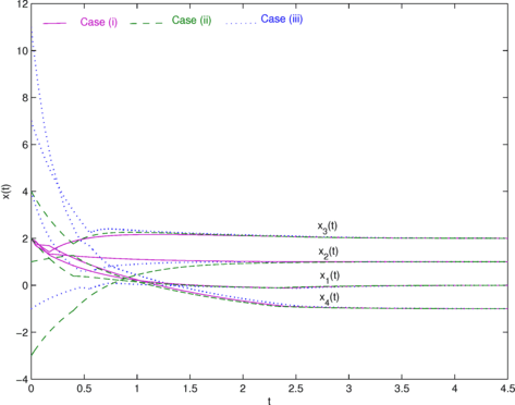

  

  Convergence to an optimal solution of problem P1, with three different initial conditions

• (ii) (2,−3,4,1), see Fig. 2 for the convergence to an optimal solution of problem P1, plotted in green.

• (iii) (−1,4,7,11), see Fig. 2 for the convergence to an optimal solution of problem P1, plotted in blue.

Problem P2

(Constrained CB2-II)

Here, the objective function and the constraints are nonsmooth. The optimal value of the objective function for this problem is 2. We have solved the problem with three different sets of initial conditions, all of which converge to the optimal solution (1,1).

• (i) (10,−8), see Fig. 6 for the convergence to an optimal solution of problem P2, plotted in pink (solid). A solution trajectory path of the differential inclusion (5) in this case is shown in Fig. 3.

  Fig. 3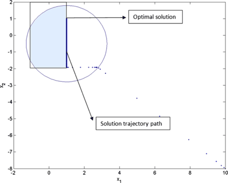

  

  Solution trajectory path of the differential inclusion (5) with initial condition (10,−8) for problem P2 and its convergence to an optimal solution, which is located on the boundary of the feasible region

• (ii) (0,−14), see Fig. 6 for the convergence to an optimal solution of problem P2, plotted in green (dashed). A solution trajectory path of the differential inclusion (5) in this case is shown in Fig. 4.

  Fig. 4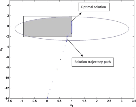

  

  Solution trajectory path of the differential inclusion (5) with initial condition (0,−14) for problem P2 and its convergence to an optimal solution, which is located on the boundary of the feasible region

• (iii) (−5,6), see Fig. 6 for the convergence to an optimal solution of problem P2, plotted in blue (dotted). A solution trajectory path of the differential inclusion (5) in this case is shown in Fig. 5.

  Fig. 5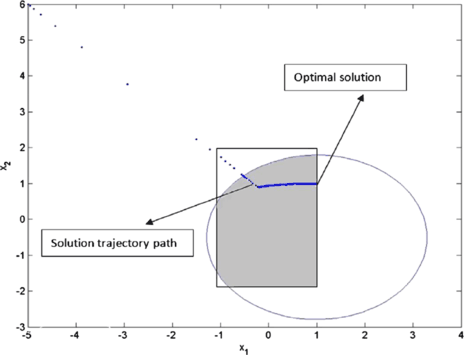

  

  Solution trajectory path of the differential inclusion (5) with initial condition (−5,6) for problem P2 and its convergence to an optimal solution, which is located on the boundary of the feasible region

  Fig. 6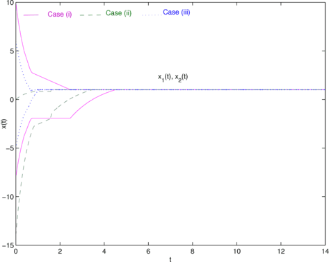

  

  Convergence to an optimal solution of problem P2, with three different initial conditions

6 Conclusions

In this paper, we introduced a differential inclusion which solves general nonsmooth convex optimization problems. Convergence to a solution was theoretically investigated. In this new neural network, the calculation of projections is not required. By the same token, there is no need to use any penalty parameter. Furthermore, this method can easily deal with infeasible starting points. We have illustrated the effectiveness of theoretical results as well as the performance of the proposed method by some numerical examples. These examples deal with nonsmooth objective functions and constraints, in which we use infeasible starting points. Some generalization of the proposed method for solving nonconvex problems and more application results will be discussed in a future work.

References

Mordukhovich, B.: Variations Analysis and Generalized Differentiation, I: Basic Theory. Springer, Berlin (2006)
Mordukhovich, B.: Variations Analysis and Generalized Differentiation, II: Applications. Springer, Berlin (2006)
Soleimani-damaneh, M.: Nonsmooth optimization using Mordukhovich’s subdifferential. SIAM J. Control Optim. 48, 3403–3432 (2010)
Shor, N.: Minimization Methods for Non-differentiable Functions. Springer, Berlin (1985)
Kelley, J.E.: The cutting-plane method for solving convex programs. J. Soc. Ind. Appl. Math. 8, 703–712 (1960)
Goffin, J.L., Haurie, A., Vial, J.P.: Decomposition and nondifferentiable optimization with the projective algorithm. Manag. Sci. 38, 284–302 (1992)
Hiriart-Urruty, J.B., Lemaréchal, C.: Convex Analysis and Minimization Algorithms: Part 2: Advanced Theory and Bundle Methods. Springer, Berlin (2010)
Solodov, M.V.: On approximations with finite precision in bundle methods for nonsmooth optimization. J. Optim. Theory Appl. 119, 151–165 (2003)
Zhao, X., Luh, P.B.: New bundle methods for solving lagrangian relaxation dual problems. J. Optim. Theory Appl. 113, 373–397 (2002)
Forti, M., Nistri, P., Quincampoix, M.: Generalized neural network for nonsmooth nonlinear programming problems. IEEE Trans. Circuits Syst. I 51, 1741–1754 (2004)
Bian, W., Xue, X.: Subgradient-based neural networks for nonsmooth nonconvex optimization problems. IEEE Trans. Neural Netw. 20, 1024–1038 (2009)
Li, G., Song, S., Guan, X.: Subgradient-based feedback neural networks for non-differentiable convex optimization problems. Sci. China Ser. F, Inf. Sci. 20, 421–435 (2006)
Li, G., Song, S., Wu, C.: Generalized gradient projection neural networks for nonsmooth optimization problems. Sci. China Ser. F, Inf. Sci. 53, 990–1004 (2010)
Lemaréchal, C., Nemirovskii, A., Nesterov, Y.: New variants of bundle methods. Math. Program. 69, 111–147 (1995)
Mäkelä, M.M.: Survey of bundle methods for nonsmooth optimization. Optim. Methods Softw. 17(1), 1–29 (2001)
Kiwiel, K.C.: Methods of Descent for Nondifferentiable Optimization. Lecture Notes in Mathematics. Springer, Berlin (1985)
Mäkelä, M.M., Neittaanmäki, P.: Nonsmooth Optimization. World Scientific, Singapore (1992)
Xia, Y., Leung, H., Wang, J.: A projection neural network and its application to constrained optimization problems. IEEE Trans. Circuits Syst. I, Fundam. Theory Appl. 49, 442–457 (2002)
Xia, Y., Wang, J.: A general projection neural network for solving monotone variational inequalities and related optimization problems. IEEE Trans. Neural Netw. 15, 318–328 (2004)
Xia, Y., Wang, J.: Neural network for solving linear programming problems with bound variables. IEEE Trans. Neural Netw. 6, 515–519 (1995)
Xia, Y.: A new neural network for solving linear programming problems and its application. IEEE Trans. Neural Netw. 7, 525–529 (1996)
Wang, J., Hu, Q., Jiang, D.: A Lagrangian network for kinematic control of redundant robot manipulators. IEEE Trans. Neural Netw. 10, 1123–1132 (1999)
Aubin, J.P., Cellina, A.: Differential Inclusion: Set-Valued Maps and Viability Theory. Springer, Berlin (1984)
Mifflin, R.: Semismooth and semiconvex functions in constrained optimization. SIAM J. Control Optim. 15, 957–972 (1977)
Defeng, S., Womersley, R.S., Houduo, Q.: A feasible semismooth asymptotically Newton method for mixed complementarity problems. Math. Program. 94, 167–187 (2002)
Clarke, F.H.: Optimization and Nonsmooth Analysis. Society for Industrial and Applied Mathematics, Philadelphia (1983)
Filippov, A.F.: Differential Equations with Discontinuous Right-Hand Sides: Control Systems. Kluwer, Boston (1988)
Hosseini, A., Hosseini, S.M., Soleimani-damaneh, M.: A differential inclusion-based approach for solving nonsmooth convex optimization problems. Optimization (2011). doi:10.1080/02331934.2011.613993
Borwein, J.M., Moors, W.B.: Essentially strictly differentiable Lipschitz functions. J. Funct. Anal. 149, 305–351 (1997)
Liu, Q., Wang, J.: A one-layer recurrent neural network for constrained nonsmooth optimization. IEEE Trans. Syst. Man Cybern., Part B 41, 1323–1333 (2011)
Lukšan, L., Vlček, J.: Test problems for nonsmooth unconstrained and linearly constrained optimization. Institute of Computer Science, Academy of Science of the Czech Republic, Technical report, 798 (2000)
Acknowledgements
The authors would like to thank the editor and the reviewers of the paper for their instructive comments. Certainly, their meticulous reading and fruitful comments enriched the content and the structure of this paper.
Author information
Authors and Affiliations
Corresponding author
Rights and permissions
About this article
Cite this article
Hosseini, A., Hosseini, S.M. A New Steepest Descent Differential Inclusion-Based Method for Solving General Nonsmooth Convex Optimization Problems. J Optim Theory Appl 159, 698–720 (2013). https://doi.org/10.1007/s10957-012-0258-4
Received:
Accepted:
Published:
Issue Date:
DOI: https://doi.org/10.1007/s10957-012-0258-4