Variable order and stepsize in general linear methods

Abstract

This paper describes the implementation of a class of IRKS methods (Wright 2002). These GLM algorithms are practical with reliable error estimators (Butcher and Podhaisky, Appl. Numer. Math. 56, 345–357 2006). The current robust ODE solvers in variable stepsize as well as in variable-order mode are based upon heuristics. In this paper, we examine an optimisation approach, based on Euler-Lagrange theory (Butcher, IMA J. Numer. Anal. 6, 433–438 1986), (Butcher, Computing 44, 209–220 1990), to control the stepsize as well as the order and implement the GLMs in an efficient manner. A set of nonstiff to mildly stiff problems have been used to investigate this approach in fixed-order and variable-order modes.

Appendix

Methods.:

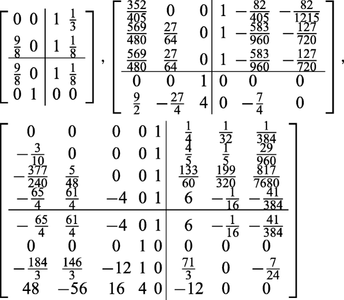
The design choices for these methods, along with the coefficients of the methods and their error estimators, are as follows:

• To use the F-property, the last abscissa c_s must be equal to 1, whereas the rest are selected at equal spacing $\frac {i}{s}$ for $i = 1,2,\dots ,s-1$.

• The error constants C_j’s for j = 1, 2, 3, 4 are $\frac {1}{8}$, $-\frac {1}{27}$, $\frac {1}{192}$ and $-\frac {19}{28125}$, respectively.

• The β values are each equal to $\frac {1}{4}$.

• The transformation matrix T = I in each possible case.

• The coefficients of the methods are as follows:

  

  

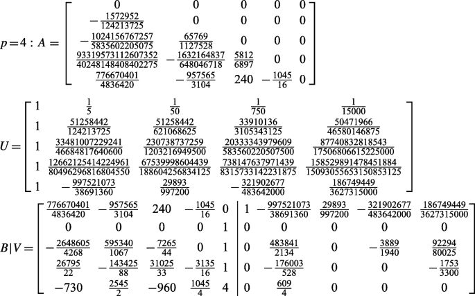
• The error estimates of the forms (7) and (8) need a set of coefficients $\left (\delta ^{\text {\tiny \textsf {T}}}, \psi , \theta \right )$ for each p.

These coefficients for the above methods are given below:

p = 1, 2.:

$\left (\left [-1, 0\right ], 1, \frac {1}{2}\right )$ and $\left (\left [\frac {255}{137},\frac {468}{137},\frac {-1701}{137}\right ], \frac {978}{137}, \frac {737}{1233}\right )$

p = 3.:

$\left (\left [-\frac {33760}{579},\frac {97984}{579},-\frac {30464}{193},\frac {23872}{579}\right ], \frac {3296}{579}, \frac {230}{579}\right )$

p = 4.:

$\left (\left [\frac {6171413506203125}{9970942359837}, -\frac {24625228556117500}{9970942359837}, \frac {36786779162438750}{9970942359837},-\frac {24323101212642500}{9970942359837},\! \frac {5929711631423125}{9970942359837}\!\right ],\!\frac {60425468695000}{9970942359837},\frac {20038565469586}{49854711799185}\!\right )$

Test problems.:

Most of these problems are taken from [2, 20], an alternative reference is mentioned otherwise. We use the interval $\left [0, 20\right ]$ for almost all the problems otherwise this is mentioned with the problem.

A2.:

A special case of the Riccatti equation:

$$y^{\prime}=-\frac{y^{3}}{2}, \hspace{1cm} y(0)= 1, $$

A3.:

An oscillatory problem (along with its 2D and 3D autonomous forms):

$$\begin{array}{l@{\hspace{1cm}}c@{\hspace{1cm}}r} \begin{array}{ccc} y^{\prime}=y\cos{(x)}, && y(0)= 1, \end{array}&\!\!\!\!\!\!\!\!\!\! \begin{array}{ccc} \begin{array}{l} y^{\prime}_{1}=y_{1}\cos{(y_{2})},\\ y^{\prime}_{2}= 1, \end{array}&& \begin{array}{l} y_{1}(0)= 1,\\ y_{2}(0)= 0, \end{array} \end{array}&\!\!\!\!\!\!\!\!\!\!\!\!\!\! \begin{array}{ccc} \begin{array}{l} y_{1}^{\prime}=y_{1}y_{2},\\ y_{2}^{\prime}=-y_{3},\\ y_{3}^{\prime}=y_{2}. \end{array} &\begin{array}{l} y_{1}(0)= 1,\\ y_{2}(0)= 1,\\ y_{3}(0)= 0. \end{array} \end{array} \end{array} $$

A4.:

A logistic curve:

$$y^{\prime}=\frac{y}{4}(1-\frac{y}{20}), \quad\quad\quad y(0)= 1, $$

B2.:

Linear chemical reaction:

$$\begin{array}{@{}rcl@{}} \begin{array}{ll} y_{1}^{\prime}=-y_{1}+y_{2}, & y_{1}(0)= 2,\\ y_{2}^{\prime}=y_{1}-2y_{2}+y_{3},& y_{2}(0)= 0,\\ y_{3}^{\prime}=y_{2}-y_{3},& y_{3}(0)= 1, \end{array} \end{array} $$

C1 (and C2).:

A radioactive decay chain of the form $y^{\prime }=Cy$ with initial vector:

$$y(0) =\left[{\begin{array}{c} 1 \\ 0 \\ {\vdots} \\ {\vdots} \\ 0\end{array}} \right], \text{where} C = \left[\begin{array}{ccccc} -1 & 0 & {\dots} & {\dots} & 0 \\ 1 & -1 & {\ddots} & & {\vdots} \\ 0 & 1 & {\ddots} & {\ddots} & \vdots\\ \vdots& {\ddots} & {\ddots} & -1 &0\\ 0 & {\dots} & 0 & 1 &0 \end{array}\right],\text{for C1, and} C = \left[\begin{array}{ccccc} -1 & 0 & {\dots} & {\dots} & 0 \\ 1 & -2 & {\ddots} & & {\vdots} \\ 0 & 2 & {\ddots} & {\ddots} & \vdots\\ \vdots& {\ddots} & {\ddots} & -9 &0\\ 0 & {\dots} & 0 & 9 &0 \end{array}\right] \text{for C2}. $$

Kepler problem.:

Kepler’s orbit equations (e is eccentricity with values 0.1, 0.3, 0.5, 0.7, 0.9):

$$\begin{array}{@{}rcl@{}} y_{1}^{\prime}&=&y_{3}, {\kern70pt} y_{1}(0)= 1-e,\\ y_{2}^{\prime}&=&y_{4},{\kern70pt} y_{2}(0)= 0,\\ y_{3}^{\prime}&=&-\frac{y_{1}}{({y_{1}^{2}}+{y_{2}^{2}})^{3/2}}, {\kern18pt}y_{3}(0)= 0,\\ y_{4}^{\prime}&=&-\frac{y_{2}}{({y_{1}^{2}}+{y_{2}^{2}})^{3/2}}, {\kern18pt} y_{4}(0)=\sqrt{\frac{1+e}{1-e}}.\\ \end{array} $$

E2.:

Van der Pol problem with $x\in \left [0, 8\right ]$.

$$\begin{array}{@{}rcl@{}} y^{\prime}_{1}&=&y_{2}, {\kern30pt} y_{1}(0)= 2,\\ y^{\prime}_{2}&=&(1-{y_{1}^{2}}){\kern9pt}y_{2}-y_{1}, y_{2}(0)= 0.\\ \end{array} $$

3-body problem.:

Here, $\mu =\frac {1}{81.45}$ and $x\in \left [0,19.14045706162071\right ]$,

$$\begin{array}{@{}rcl@{}} \begin{array}{ll} y_{1}^{\prime}=y_{4},&y_{1}(0)= 0.994,\\ y_{2}^{\prime}=y_{5},&y_{2}(0)= 0,\\ y_{3}^{\prime}=y_{6},&y_{3}(0)= 0,\\ y_{4}^{\prime}= 2y_{5}+y_{1}-\frac{\mu \left( y_{1}+\mu-1\right)}{({y_{2}^{2}}+{y_{3}^{2}}+\left( y_{1}+\mu-1\right)^{2})^{3/2}} \\\quad\quad -\frac{\left( 1-\mu\right)\left( y_{1}+\mu \right)}{({y_{2}^{2}}+{y_{3}^{2}}+\left( y_{1}+\mu-1\right)^{2})^{3/2}},& y_{4}(0)= 0,\\ y_{5}^{\prime}=-2y_{4}+y_{2}-\frac{\mu y_{2}}{({y_{2}^{2}}+{y_{3}^{2}}+\left( y_{1}+\mu-1\right)^{2})^{3/2}}\\\quad\quad -\frac{\left( 1-\mu \right)y_{2}}{({y_{2}^{2}}+{y_{3}^{2}}+\left( y_{1}+\mu-1\right)^{2})^{3/2}}, &y_{5}(0)=-2.0015851063790825224,\\ y_{6}^{\prime}=-\frac{\mu y_{3}}{({y_{2}^{2}}+{y_{3}^{2}}+\left( y_{1}+\mu-1\right)^{2})^{3/2}}\\\quad\quad -\frac{\left( 1-\mu \right)y_{3}}{({y_{2}^{2}}+{y_{3}^{2}}+\left( y_{1}+\mu-1\right)^{2})^{3/2}}& y_{6}(0)= 0. \end{array} \end{array} $$

HO.:

Harmonic oscillator:

$$\begin{array}{@{}rcl@{}} y^{\prime}_{1}&=&-y_{2}, {\kern20pt} y_{1}(0)= 0,\\ y^{\prime}_{2}&=&y_{1}, {\kern28pt}y_{2}(0)= 1. \end{array} $$

Bubble.:

A model of cavitating bubble:

$$\begin{array}{@{}rcl@{}} \begin{array}{ccc} \begin{array}{l} \frac{dy_{1}}{dx}=y_{2},\\ \frac{dy_{2}}{dx}=\frac{5\exp{\left( \frac{-x}{x^{*}}\right)}-1-1.5{y_{2}^{2}}}{y_{1}}-\frac{ay_{2}+D}{{y_{1}^{2}}}+\frac{1+D}{y_{1}^{3\gamma+ 1}},\\ x^{*}=\frac{0.029}{R_{0}},\quad a=\frac{4\times 10^{-5}}{R_{0}},\quad D=\frac{1.456 \times 10^{-4}}{R_{0}},\quad\gamma= 1.4,\hspace{3mm}R_{0}= 10^{-3}. \end{array} && \begin{array}{l} y_{1}(0)= 1,\\ y_{2}(0)= 0. \end{array} \end{array} \end{array} $$

PR.:

This problem is used to examine the stability behaviour of the numerical methods:

$$y^{\prime}=\lambda (y-f(x))+f^{\prime}(x), $$

with true solution y(x) = f(x) and y(0) = 1. Here, two cases are considered: (i) $f(x)=\exp {(\mu x)}$ with λ = − 0.1 and μ = − 0.1 and (ii) $f(x)=\sin {(x)}$ with λ = − 4.

mild1.:

Butcher [8] with $y(0)=\left [1,0\right ]^{\text {\tiny \textsf {T}}}$ and $x\in \left [0,\pi \right ]$.

$$\begin{array}{@{}rcl@{}} y^{\prime}_{1}&=&-16y_{1}+ 12y_{2}+ 16\cos{(x)}-13\sin{(x)},\\ y^{\prime}_{2}&=&12y_{1}-9y_{2}-11\cos{(x)}+ 9\sin{(x)}. \end{array} $$

References

Ahmad, S.: Efficient implementation of implicit Runge–Kutta methods. Masters thesis, The University of Auckland. This can be provided on demand by the author (sahm056@aucklanduni.ac.nz) (2011)
Ahmad, S.: Design and construction of software for general linear methods, PhD thesis, Massey University, Auckland, https://mro.massey.ac.nz/handle/10179/9925(2016)
Butcher, J.C.: Optimal order and stepsize sequences,. IMA J. Numer. Anal. 6, 433–438 (1986)
Butcher, J.C.: Order, stepsize and stiffness switching. Computing 44, 209–220 (1990)
Butcher, J.C.: General linear methods for the parallel solution of ordinary differential equations. World Sci. Ser. Appl. Anal. 2, 99–111 (1993)
Butcher, J.C.: An introduction to DIMSIMs. Comput. Appl. Math. 14(1), 59–72 (1995)
Butcher, J.C.: General linear methods for stiff differential equations. BIT 41 (2), 240–264 (2001)
Butcher, J.C.: Numerical methods for ordinary differential equations. Wiley, Chichester (2016)
Butcher, J.C.: Thirty years of G–stability. BIT 46, 479–489 (2006)
Butcher, J.C., Chartier, P., Jackiewicz, Z.: Experiments with variable–order type 1 DIMSIM code. Numer. Algorithms 22, 237– (1999)
Butcher, J.C., Podhaisky, H.: On error estimation in general linear methods for stiff ODEs. Appl. Numer. Math. 56, 345–357 (2006)
Butcher, J.C., Jackiewicz, Z.: A new approach to error estimation for general linear methods. Numer. Math. 95, 487–502 (2003)
Butcher, J.C., Jackiewicz, Z., Wright, W. M.: Error propagation for general linear methods for ordinary differential equations. J. Complexity 23, 560–580 (2007)
Butcher, J.C., Wright, W.M.: The construction of practical general linear methods. BIT 43, 695–721 (2003)
Butcher, J.C., Wright, W.M.: Application of doubly companion matrices. Appl. Numer. Math. 56, 358–373 (2006)
Gladwell, I., Shampine, L.F., Brankin, R.W.: Automatic selection for the initial stepsize for an ODE solver. J. Comput. Appl. Math. 18, 175–192 (1987)
Gustafsson, K., Lundh, M., Söderlind, G.: A PI stepsize control for the numerical solution of ordinary differential equations. BIT 28, 270–287 (1988)
Hairer, E., Wanner, G.: Stiff differential equations solved by Radau methods. J. Comput. Appl. Math. 111, 93–111 (1999)
Hairer, E., Wanner, G.: Solving ordinary differential equations II. Springer, Berlin (1996)
Hull, T.E., Enright, W.H., Fellen, B.M., Sedgwick, A.E.: Comparing numerical methods for ordinary differential equations. SIAM J. Numer. Anal. 9(4), 603–637 (1972)
Jackiewicz, Z.: General linear methods for ordinary differential equations. Wiley, Chichester (2009)
Shampine, L.F., Gordon, M.K.: Using DE/STEP, INTRP to Solve Ordinary Differential Equations, United States: N. p. Web (1974)
Wright, W.M.: General Linear Methods with Inherent Runge–Kutta Stability. PhD thesis, The University of Auckland (2002)
Author information
Authors and Affiliations
Corresponding author
Additional information
Publisher’s note
Springer Nature remains neutral with regard to jurisdictional claims in published maps and institutional affiliations.