
Abstract
Tag collision is a pressing issue in radio frequency identification systems which significantly lowers the system performance if not mitigated carefully. This paper presents the Monte–Carlo Query Tree Search (MCQTS) method as a novel and fast anti-collision algorithm. This method combines the capabilities of the conventional Monte–Carlo Tree Search and Query Tree by applying a few heuristics on the tree traversal to raise the chance of facing the most promising states. The collision mitigation based on the MCQTS is presented and its performance in terms of time, and space (memory) complexity is analytically verified. Simulations are performed, and the effects of tree size, number of tags, and tag ID length on the performance of the proposed method are investigated. The results are compared to the previously presented tree-based algorithms, and it is shown that for typical tag lengths, the MCQTS method performs between 3.89% and 62.06% (in average) faster than the conventional methods for multi-tag identification.
1 Introduction
Nowadays, automatic identification of objects and individuals, and collecting data related to them without the necessity of human intervention is in high demand in many sectors such as industry, market, medicine, and finance [1, 2]. Several technologies have been designed and implemented so far to meet these needs. Barcodes, smart cards, optical character recognition (OCR), biometrics, and radio frequency identification (RFID) are some examples in this regard among which, the latter is the most dominant and has attracted a great deal of interest over the past decade [3,4,5].
RFID works wirelessly and is capable of identifying target objects by means of a reader device and an electronic tag which is usually attached to the object. Identification is completed when the reader successfully collects the tag ID via radio frequency data transmission. In some cases, it may forward the tag ID to a back-end system for storage and analysis [6]. This process is depicted in Fig. 1. Because of the reliability, flexibility, cost-efficiency, and long service life of RFID-based solutions [7], they are now ubiquitous in many domains such as contactless payment [8,9,10], customer behavior identification [11,12,13], product manufacturing [14,15,16,17,18], healthcare [19,20,21,22,23], access management [24,25,26,27], logistics management [28,29,30,31], and transportation [32,33,34] to name a few.

The RFID working mechanism
However, RFID networks often suffer from the serious issue of “tag collision” which degrades their performance [35, 36]. Collision happens when multiple tags are transmitting simultaneously to the reader within its interrogation zone (Fig. 2). Such an interference confuses the reader, resulting in incorrect identification of the tags. Tag starvation is a common consequence in this situation where the reader fails to identify a tag for a long time due to involving in endless collisions.

Diagram of tag collision problem in the identification range of a reader
A number of RFID anti-collision algorithms have been proposed to tackle the tag collision problem. These algorithms are designed to achieve an efficient tag reading rate. The time division multiple access (TDMA)-based anti-collision protocols are more frequently used because of their robustness and easy implementation [37]. TDMA-based algorithms are mainly divided into two categories: tree-based (deterministic) methods [38,39,40,41,42] and ALOHA-based (probabilistic) methods [43,44,45,46]. The deterministic algorithms such as collision tree (CT) [47,48,49], query tree (QT) [50,51,52,53,54], binary search (BS) [37, 55,56,57,58] and bit-locking back-off (BLBO) [59] ensure the identification of all tags in range, but often fail to achieve a low communication overhead. On the other hand, ALOHA-based algorithms as in [60, 61] are simple and fast, but suffer from the tag starvation problem.
Despite the versatility of the tree-based algorithms, all of them use conventional search methods to reduce the required computational power. Nevertheless, with the recent introduction of low-cost, high-power embedded computing systems (e.g. ESP8266, Raspberry Pi), it is now possible to consider the heuristic search algorithms, such as the best-first search, the A* algorithm, simulated-annealing, genetic algorithms [62], and the Monte–Carlo Tree Search (MCTS) [63], in order to design more efficient RFID anti-collision systems.
In this paper, we present the incorporation of a novel modified version of the MCTS into the QT algorithm. The new algorithm is compared to the previously reported methods, and its effectiveness for RFID collision mitigation is investigated. The paper is organized as follows: Sect. 2 describes the MCTS and QT as heuristic and non-heuristic conventional search algorithms, respectively, as they are the building blocks of the new anti-collision algorithm. Section 3 introduces the idea of combining the MCTS and QT to benefit from the best of both worlds. The novel anti-collision protocol, as well as a simple trick to reduce its computation costs, are then introduced, and described in detail. Section 4 presents the time, and space complexity analyses of the proposed method as well as the results of simulations which are compared to some of the current tree-based algorithms. Finally, Sect. 5 concludes the paper.
2 Conventional search algorithms
The core of a tree-based anti-collision algorithm is the search procedure that is used to explore the search tree, i.e., the data structure formed by the tags’ IDs. Search algorithms can be categorized into two types: heuristic and non-heuristic. A heuristic search strategy aims to optimize a problem by iteratively improving the solution based on a heuristic function (cost measure) [64]. In contrast to non-heuristic search algorithms, which follow deterministic routines towards an optimal solution, heuristic algorithms are not always guaranteed to find an optimal solution, hence terminating at a suboptimal point. However, the solution is found faster and with less memory requirements. In this section, the MCTS and the QT are briefly introduced, as a random-heuristic search algorithm, and a deterministic and non-heuristic one, respectively. These algorithms construct the very first building blocks of the new anti-collision scheme which will be presented in Sect. 3.
2.1 Monte–Carlo tree search
MCTS [65] is one the most popular planning algorithms which have been used as a reliable decision-making method in many perfect information games (e.g., Google DeepMind’s AlphaGo [66]). In addition to being extraordinarily successful in the field of game playing, MCTS can be a suitable solution for other types of problems, specifically, the ones that can be characterized from the perspective of “states” and “actions”. The primary purpose of MCTS is to discover the most promising actions in order to reach the most promising states based on the results of the random simulations, i.e., playouts. A playout is the action of tree traversing in which the moves are selected randomly (or pseudo-randomly), starting from a root node to a terminal state. Final results of the playout are used to update the statistics of the game tree nodes along the simulation path. These statistics are then used to take subsequent actions such that they would be most likely to result in a win or a desirable terminal state.
The number of iterations in the MCTS depends on the complexity of the task to be completed as well as the computational capacity, e.g., number of processor cores. There are four phases in each iteration that fulfill the search procedure [67]:
-
Selection phase Start from the root node S0, recursively advance to the selected child nodes one by one until a leaf node (i.e., a node with no children) is reached.
-
Expansion phase If the leaf node does not satisfy the terminal condition of the game, add a new child node into the tree for each available action from the game position, and randomly select one of them, and label it as C.
-
Simulation phase Initiate a playout from C, and walk down the tree until a terminal state is reached, and the game result is concluded.
-
Backpropagation phase Update the statistics associated with all of the visited nodes during the iteration, except for the ones on the simulation path (i.e., from S0 to C).
Two statistics must be stored for each node: (a) the number of times that it has been visited, and (b) total playout reward, i.e., the number of times that simulations passed through that node has resulted in a win. These four phases are run repeatedly for a desired period of time; eventually, once the MCTS procedure is finished, the best path to move through is the one whose nodes are visited the most.
The core part of the MCTS is the action selection strategy (tree policy) for the selection phase. It is commonly a function of the node statistics, and the child node that maximizes its value is selected to traverse through in the selection phase. In essence, we are willing to select not only the moves that have a higher chance of winning but also the ones which are not explored enough during the iterations of the algorithm. Therefore, we are facing the so-called exploration–exploitation dilemma, that is the problem of balancing exploration and exploitation between multiple options, each with an unknown payout, and the goal is to determine the best moves to achieve the highest expected gain. This is the main challenge of multi-armed bandit (MAB) problem which is a classic reinforcement learning (RL) problem.
One of the solutions to the MAB problem is the Upper Confidence Bound 1 (UCB1) which is called the UCT (Upper Confidence bound 1 applied to Trees) when applied to the MCTS [68]. The UCT is a value-based RL algorithm and its action selection function is given by
where \(v_{i}\) is the total simulation reward of the child node i, \(n_{i}\) is the total number of visits to the child node i, and \(N = \sum\nolimits_{j} {n_{j} }\) is the total number of simulations. \(c\) is a constant value which adjusts the balance between exploitation and exploration, and is analytically proven to be equal to \(\sqrt 2\) [68]; however, it can be chosen according to the nature of the problem.
The MCTS can be easily implemented and it operates effectively with no prior knowledge. The search tree in MCTS grows asymmetrically as the explorations become concentrated on the more promising subtrees. This is due to the RL-based nature of the UCT, which leads MCTS to achieve better results than the classical algorithms for games with high branching factors. Furthermore, it is possible to interrupt MCTS at any time to yield the most promising move already found. A disadvantage of the MCTS is its high memory requirements due to the rapid growth of the search tree after the first few iterations.
2.2 Query tree
QT algorithm [50] follows a request-response routine between the reader and the tags, which can be represented in the form of a full \(m\)-ary tree. In each interrogation, the reader transmits a query including a binary string which is called a prefix. After receiving the reader’s query command, every tag within the effective identification range of the reader, compares the prefix with its ID to acknowledge whether it matches the front part (left side) of the ID. In case of a match, the tag transmits the remaining of its ID back to the reader; otherwise, it waits for the next query.
There are three cases which may occur after reader’s query: (1) only one tag responds to the reader’s query; thus, the query leads to the successful identification of that readable tag. (2) there is no match for the transmitted prefix and no tag responds to the reader, which is an idle state, and (3) there may be two or more responses from the tags to the reader which is a collision. If a collision occurs, the reader appends an \(\ell\)-bit binary string to the current prefix, and queries for the new prefix. This will introduce \(m = 2^{\ell }\) new child nodes into the search tree, and the reader will search for them respectively. \(m\) is the branching factor of the tree, and such a tree structure is called binary tree for \(\ell = 1\), quadtree for \(\ell = 2\), octree for \(\ell = 3\), and \(m\)-ary tree in general. The reader continues this procedure until one tag is successfully identified. It then sends a command to put the identified tag into the halt state. Afterward, the reader starts a new set of queries with other prefixes and looks for other tags, and it stops when all of the tags are identified.
Take for example a network with four tags, which their unique IDs are: 1001, 0010, 1011, and 1000. If we use the binary tree, we will encounter three collision nodes, one idle node, and four readable nodes. The QT for this network is shown in Fig. 3.

An example of binary QT for a network with four tags: 1001, 0010, 1011, and 1000
QT algorithm is simple, easy-to-implement, and imposes minimal computational and memory requirements on tags. In fact, each tag is memoryless (i.e., only its ID needs to be stored), just comparing its ID with the reader’s query [50]. Thus, the hardware cost is low. However, the performance of the QT algorithm is greatly affected by the distribution of the tags’ IDs due to the mechanical update routine of the query prefix. As a consequence, QT produces a large number of idle timeslots.
3 Monte–Carlo query tree search
Although heuristic search algorithms are capable of handling complex problems, they have not been used for anti-collision schemes so far. This is probably due to their sub-optimality and the tendency of the RFID community to employ the classical search algorithms. For the case of the RFID anti-collision schemes, even a non-heuristic algorithm should be deterministic in order to guarantee the successful identification of all tags. However, the high computational overhead of non-heuristic algorithms might become an issue. One can consider a combination of heuristic and non-heuristic search strategies as a possible solution to the multiple tag identification for RFID systems to benefit from the optimality of the former and the acceptable time complexity of the latter.
The main idea behind the proposed method is to fit QT to the search tree of the tag identification problem, and use a modified version of MCTS to explore it. In this way, we can have the memoryless nature of the QT as well as its optimality, and improve the tree exploration by leveraging RL-based nature of the MCTS. We propose a new variant of MCTS, aiming to emphasize the actions that lead to finding uninvestigated or collision nodes (which will be called valuable nodes, from now on), and penalize those of which approach idle nodes. This strategy has two advantageous outcomes: (1) by shrewdly passing through valuable nodes, we aim to reach readable nodes in the deeper layers of the tree, and (2) at the same time, we eliminate the idle timeslots of the reader’s interrogation by avoiding the idle nodes.
In this work, we have viewed the tag identification as a single-player deterministic game in order to learn the best actions by which we can win the game, i.e., successfully identify all of the available tags, as quick as possible. We represent the entire process in the form of a tree data structure in which each node corresponds to the action of appending an \(\ell\)-bit code from the set \(\left\{ {0 \cdots 00,0 \cdots 01, \cdots ,1 \cdots 11} \right\}\) to the current prefix in QT. By employing MCTS with a new upper confidence bound strategy, a reward is given to the appending actions that lead to valuable nodes, since they are the ones which should be explored further. Tag identification is performed by exploring the search tree based on the modified MCTS algorithm, and the conduction of the QT routine when passing each node. Next decisions are made based on the performance of the previous actions. Eventually, all the tags will be identified after a number of iterations of this Monte–Carlo Query Tree Search (MCQTS) algorithm.
While using MCTS necessitates postponing the actual tag reading until the end, the proposed method (MCQTS) manages to do this during the Monte–Carlo iterations. Therefore, the simulation (playout) phase plays a significant role in the tag identification, and improving its efficiency is of paramount importance. We propose the following modifications to the MCTS for the purpose of devising an effective search:
-
1.
In order for the game actions to quickly converge to the optimal ones, the statistics of the nodes visited during the simulation are also recorded. To this end, two arrays are set to store \(n_{i}\) and \(v_{i}\) values, each with a length of
$$L = \sum\limits_{i = 0}^{D} {m^{i} } = \sum\limits_{i = 0}^{D} {2^{\ell i} }$$(2)where \(m\) and \(\ell\) are the same as in QT, and \(D\) is the maximum depth of the tree which is given by:
$$D = \left\lceil {\frac{K}{\ell }} \right\rceil$$(3)where \(K\) is the length of the tag ID and \(\left\lceil . \right\rceil\) is the ceiling function.
-
2.
A “reward and punishment” scheme is adopted to keep the score throughout the game. The paradigm for such a scheme is demonstrated in Fig. 4. The tag identification is best done when the idle nodes are avoided the most, and the valuable nodes are explored quicker. As a result, an action is rewarded if it leads to discovering valuable nodes, and punished otherwise. The reward is given in the form of a unit increment in the reward value (\(v_{i}\)) of some associated nodes.
-
3.
The terminal state of the game is determined to be either a readable node or an idle node which is treated with punishment once it is reached. If the path from S0 to the parent node of an encountered terminal node contains at least one collision node, every node along the path is rewarded. This is because we intend to further investigate such a path as it has a high chance of having undiscovered readable nodes. In addition, we set an array \(\omega\) (with the length \(L\)) to store the status of nodes. The ith element of \(\omega\) (\(\omega_{i}\)), takes the values 0, 1, 2, and 3 for uninvestigated, collision, idle, and identified nodes, respectively. Each \(\omega_{i}\) is initially set to zero before the reader’s interrogation, and takes a status value once the reader’s query for the prefix of the ith node is finished.
-
4.
The indices of the nodes are assumed to start from zero (corresponding to the initial state S0), and incremented by one for successive nodes, which are ordered ascendingly by their associated prefix in each layer. Hence, the indices of the children of the ith node in the tree are: \(\left\{ {2^{\ell } i + j} \right\}_{j = 1}^{{2^{\ell } }}\). We define a zero–one status function as
$$\phi \left( i \right) = \left\{ {\begin{array}{*{20}c} 1 & {\omega_{i} = 0,1} \\ 0 & {otherwise} \\ \end{array} } \right.$$(4)where \(\phi \left( i \right)\) is equal to one for all valuable nodes, and zero otherwise. Let \(\alpha \left( {j|i} \right)\) be the action of selecting a child node j, given that the algorithm is at the ith node. Thus, the probability of each random action in the playout is given by
$$\Pr \left( {\alpha \left( {j|i} \right)} \right) = \frac{1}{{\sum\limits_{{k = 2^{\ell } i + 1}}^{{2^{\ell } (i + 1)}} {\phi (k)} }}$$(5)which is uniformly randomly distributed. By using the status function, we penalize the ith node once for each action \(\alpha \left( {j|i} \right)\) if all of the children of the node are either already identified or idle. For this, the reward value of the ith node is decremented by one.
-
5.
A constraint is put on the choice of j in \(\alpha \left( {j|i} \right)\) so that the playouts are selected randomly from a set of valuable child nodes, so that the nodes that have been identified before, or are idle, are not considered as the possible paths to move through. We make a minor modification in the original UCT formula (Eq. 1) and propose a new function, given by
$$UCT_{MCQTS} (i) = \phi (i)\left( {\frac{{v_{i} }}{{n_{i} }} + 2\sqrt {\frac{{\ln n_{p(i)} }}{{n_{i} }}} } \right)$$(6)where \(c = 2\) is chosen empirically, and \(p(i) = \left\lfloor {\frac{i - 1}{m}} \right\rfloor\) gives the index of the parent of the ith node. Here, we have used the number of visits to the parent node of the competing child nodes (\(n_{p(i)}\)) instead of using the total number of playouts (\(N\)) to take a more local decision. Furthermore, we have multiplied the UCT formula by the status function to ensure that the idle or identified nodes are not involved in the action selection. Such a tree policy ensures that the need for exploring the useless parts of the search tree during the simulations, is eliminated.
Fig. 4 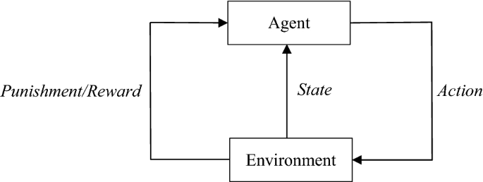
Reward and punishment scheme

Having applied the aforementioned modifications, we exploit the algorithm to recognize the tags in the network. The complete flowchart of the MCQTS is depicted in the Fig. 5. Obviously, the \(UCT_{MCQTS}\) values must be computed for some nodes in each iteration, which might be computationally demanding and slow down the identification process. A simple yet effective way to reduce the computation costs is to use look-up tables (LUTs) to store the results of some frequent computations. According to Eq. (6), the first term in the parenthesis is the number of a node visits divided by its reward value. The most frequent pairs of \(\left( {v_{i} ,n_{i} } \right)\) occurred in the iterations usually correspond to the nodes that are located at the upper layers of the tree, such as (0, 0), (0, 1), (1, 2), …, and (1, \(2^{\ell }\)). Nevertheless, these pairs can be chosen according to the specified network. Thus, we can construct a small LUT to store the calculated values of \({{v_{i} } \mathord{\left/ {\vphantom {{v_{i} } {n_{i} }}} \right. \kern-\nulldelimiterspace} {n_{i} }}\) for each pair, and use it in \(UCT_{MCQTS}\) computations. This simple trick has a considerable effect on the energy efficiency of the algorithm.

Flowchart of the MCQTS algorithm
4 Performance analysis
4.1 Time complexity
Time complexity of an anti-collision algorithm is defined as the number of required query cycles in a complete round of the recognition of a set of tags. It is commonly expressed as a function of the number of tags to be identified, as well as in the form of the big O notation. Here, we first derive the time complexity of the modified MCTS and use it in tandem with that of the QT to derive the time complexity of the proposed MCQTS.
Deriving the time complexity of the original MCTS is straightforward. MCTS executes four phases for, say \(N_{I}\), iterations. Therefore, we can express the overall time complexity as:
where \(t_{s}\), \(t_{e}\), \(t_{p}\), and \(t_{b}\) are the contributions of the running times of selection, expansion, simulation, and backpropagation phases, respectively. Since \(m\) nodes in every layer are involved in the selection phase, this phase runs in \(O(mD)\); hence, \(t_{s} = mD\). Expansion phase takes constant time (\(O(1)\)) as it just adds a number of child nodes to the tree; hence \(t_{e} = 1\). Simulation and backpropagation take time proportional to the depth of the tree, i.e. \(O(D)\); hence \(t_{p} = t_{b} = D\). The worst-case corresponds to simulation from S0 or the backpropagation from a leaf node in the last layer. Substituting the results in Eq. (7), we obtain the time complexity of the MCTS:
By adopting the tree policy of Eq. (6), only valuable nodes are involved in the action selection. Thus, the selection phase of the modified MCTS runs in \(O(\widehat{m}D)\) with \(\widehat{m} \le m\). A reasonable choice for \(\widehat{m}\) is the expected number of valuable nodes in the tree (\(E\left[ {\phi (i)} \right]\)); however, we rather use its upper bound (\(m\)) as we are interested in the worst-case scenario. If we assume not every node is assigned to a tag, it is possible to have some nodes at last layers with more than one idle child. Such nodes may not be discovered in a single iteration. Thus, it is reasonable to say
where \(\gamma\) is an efficiency coefficient, which is a measure of how well the algorithm operates, i.e., how quickly it identifies all of the tags. A large \(\gamma\) corresponds to smaller number of iterations, lower computation cost, and higher speed. In practice we do not expect \(\gamma\) to be smaller than 0.5 (typically); however, this must be ensured through evaluations. One can easily deduce that the efficiency coefficient is strongly dependent on the way the tree is traversed during the tag identification. In fact, the purpose of the rules we established for tree traversal in Sect. 3, was to achieve values of \(\gamma\) as close as possible to 1. Substituting Eq. (9) in Eq. (8) and using the upper bound of \(\widehat{m}\), we obtain:
Since \(D = \left\lceil {\frac{K}{\ell }} \right\rceil \le \frac{K}{\ell } + 1\), we can rewrite Eq. (10) as follows:
Equation (11) presents the worst-case time complexity of the modified MCTS.
On the other hand, according to [50], the average time complexity of the QT algorithm is given by:
while its worst-case time complexity is as follows:
Although the worst-case complexity of Eq. (13) looks complicated, it is proved in [50] that the QT has high probability of having linear running time (\(O\left( {N_{t} } \right)\)). In fact, the authors showed the probability that QT takes at least \(cN_{t}\) steps to identify \(N_{t} \ge 2\) tags is at most \(\exp \left( { - 0.4N_{t} ({c \mathord{\left/ {\vphantom {c 2}} \right. \kern-\nulldelimiterspace} 2} - 2)} \right)\) which decreases exponentially as \(N_{t}\) increases. Thus, we assume \(O\left( {N_{t} } \right)\) for the running time of the QT, and combine it with the time complexity of the modified MCTS to obtain the overall time complexity of the MCQTS in the worst-case scenario:
where \({{mK} \mathord{\left/ {\vphantom {{mK} \ell }} \right. \kern-\nulldelimiterspace} \ell }\) is regarded as constant and omitted as for a fixed network architecture. Hence, MCQTS takes linear time. However, the complexity of MCQTS is greatly influenced by the value of \(K\) due to the nature of QT, and care should be taken with the choice of the ID length when using MCQTS. Large values of \(K\) (e.g. 96 or 198 for EPC Global tags), and small values of \(\ell\), results in an additional computational overhead by increasing the depth of the tree, and changing the time complexity (see Eqs. 10, 11). Note that the time complexity is not the only issue in this situation, since a large \(K\) (or small \(\ell\)) also results in higher space complexity due to the dramatic increase of \(L\), which will be discussed in Sect. 4.2.
Table 1 compares the time complexity of MCQTS to five other tree-based algorithms: BS [35], QT [50], CT [47, 48], BLBO [59], and the proposed method in [61] (which we shall call CQT, since it is based on compressed query tree), according to [69]. As can be seen from Table 1, CT, BLBO and CQT take linear time and their complexities is only affected by the number of tags, regardless of the ID length. Time complexity of the BS does not depend on ID length either; however, the existence of \(N_{t} !\) inside the big O notation makes it less efficient than others. We argue that the MCQTS belongs to the class of linear time anti-collision algorithms if the ID length is not very long, and inherits this feature from its ancestor (QT), which has linear running time with high probability. Nevertheless, this does not make it quite equivalent to CT, BLBO, and CQT for which the time complexities are given by:
showing linear time dependency, regardless of the ID length. The time complexities of other tree-based algorithms such as multi-bit identification collision tree (MICT) [49], and improved quad-tree (IQT) [42] lie somewhere in between the mentioned ones in Table 1. MICT is a CT-based scheme and its time complexity is given by:
where \(\ell\) is the length of the query prefix. It has been proved in [49], that for \(\ell \ge 2\), the time complexity of the MICT is lower than that of CT. IQT, on the other hand, is a modified form of quadtree search and its time complexity is given by:
IQT is superior to the original quadtree search and BS, as it can eliminate the idle timeslots of the tag identification.
4.2 Space complexity
Space (memory) complexity of an anti-collision algorithm is defined as the size of the memory (in bits) required for the reader during the tag identification. Similar to the time complexity, we derive the space complexity of the MCQTS in terms of big O notation to see how much the required storage grows, in the worst case, as \(N_{t}\), \(K\), or \(\ell\) increase. As with the time complexity formula, we derive the space complexity of the MCQTS by firstly deriving the space complexity of the modified MCTS, and combining it with that of the QT.
The proposed variant of MCTS requires three arrays to store the values of \(\left\{ {\omega_{i} } \right\}_{i = 1}^{L}\), \(\left\{ {n_{i} } \right\}_{i = 1}^{L}\), and \(\left\{ {v_{i} } \right\}_{i = 1}^{L}\). \(b_{1}\), \(b_{2}\), and \(b_{3}\) are defined as the required number of bits to store \(\omega_{i}\), \(n_{i}\), and \(v_{i}\) in the memory, respectively. We express the space complexity using the contribution of these arrays:
Each \(\omega_{i}\) can take four different values (\(\omega_{i} \in \left\{ {0,1,2,3} \right\}\)), hence it can be represented with a 2-bit code, i.e., \(b_{1} = 2\). Apart from the S0, the following inequality holds for the maximum number of visits to a node:
where the upper bound corresponds to the maximum number of simulations of a child node. By assuming the upper bound of Eq. (19), and taking \(\left\lceil {{L \mathord{\left/ {\vphantom {L m}} \right. \kern-\nulldelimiterspace} m}} \right\rceil \approx {L \mathord{\left/ {\vphantom {L m}} \right. \kern-\nulldelimiterspace} m}\) for the sake of simplicity, at most \(b_{2} = \left\lceil {\log_{2} ({L \mathord{\left/ {\vphantom {L m}} \right. \kern-\nulldelimiterspace} m})} \right\rceil\) bits are required to store each \(n_{i}\) value. On the other hand, as the reward and punishment rules of the MCQTS cancel out each other most of the times, the value of \(v_{i}\) is always (much) less than the upper bound of Eq. (19); hence: \(b_{3} < b_{2}\). Thus, \(b_{2} L\) is the most significant term in Eq. (18), and the worst-case space complexity of the modified MCTS becomes:
Space complexity of the QT in the worst-case scenario is \(O(2^{K} K)\), since the maximum size of each query prefix is \(K\) bits, and the maximum number of queries is \(2^{K}\) [61]. By integrating the two space complexities, we obtain the worst-case reader-side space complexity of the MCQTS as:
Equation (21) reveals that although the MCQTS has fine performance in terms of time complexity, the amount of memory required to run the algorithm is rather high. Increasing the length of the tag ID can further exacerbate the problem. As discussed in Sect. 2.1, the drawback of the MCTS is its high memory demand, and the MCQTS has inherited it to some extent. Overall, it can be said that the MCQTS is more memory-efficient for the tags having smaller ID length.
We analyze the memory requirements of the MCQTS in two different scenarios: \(K = 10,\ell = 1\) as a typical scenario and \(K = 24,\ell = 4\) as a more complicated one. If we neglect \(b_{3}\), the RFID reader will require approximately 4.3 kilobytes for the first scenario and approximately 101.8 megabytes for the second one. We argue that both scenarios can be tolerated by low-cost, high-power embedded computing systems as RFID readers. For instance, a low cost ESP8266 module, e.g., ESP-01, can handle the first scenario, and even the obsolete generations of Raspberry Pi, e.g., Pi 1 Model A and Pi 1 Model B, could handle the second scenario, not to mention the recent releases.
4.3 Simulation
Besides the theoretical analysis, simulations are performed to obtain more realistic performance measures of the proposed method. To this end, we have implemented the QT via computer programming in which every node has been represented by its corresponding \(\ell\)-bit binary string (see Fig. 3). After writing the simulation codes of the proposed modified MCTS, we run it together with that of QT to simulate the MCQTS. No special toolboxes or libraries used for simulation, only normal programming scripts. It is worth noting that the random playouts were implemented using pseudo-random number generators, initialized with simple seeds such as the CPU clock or the current time.
We have simulated the MCQTS algorithm with different values of \(\ell\) to assess its performance in tag identification. The performance is expressed in terms of the number of query cycles needed to identify a maximum number of 500 tags. Figure 6 shows the simulation results of the MCQTS with \(\ell = 1\) (binary-MCQTS), \(\ell = 2\) (quad-MCQTS), \(\ell = 3\) (oct-MCQTS), and \(\ell = 4\) (hex-MCQTS), with a same ID length in every case. The data points in the curves are the average values of 50 simulations. According to (2) and (3), if \(K\) is fixed, the depth of the search tree as well as the total number of the nodes (\(L\)) decreases with the increase of \(\ell\) and thereby the tree shrinks and becomes shallower. In such a case, the MCQTS deals with a simpler search tree and hence the tag identification can be performed faster. This can be ensured from the simulation results depicted in Fig. 6. The hex-MCQTS completes the tag identification in 560 query cycles, while oct-MCQTS, quad-MCQTS, and binary-MCQTS require 684 and 1215 query cycles, respectively. Note that although incrementing the value of \(\ell\) beyond 4 (which increases the branching factor, i.e., \(m = 2^{\ell }\)) leads to simpler search spaces, the selection phase of the Monte–Carlo iterations becomes more challenging due to the generation of more competing child nodes. Hence, performance improvement is not always guaranteed. In the MAB sense, increasing the branching factor is equivalent to increasing the number of arms, making the resource (playout) allocation harder. Moreover, the choice of \(\ell\) also depends on the number and the ID length of the tags we want to reside in the network.

Comparison of identification delay of the MCQTS with \(\ell = 1\), \(\ell = 2\), \(\ell = 3\), and \(\ell = 4\) based on the query cycles
One way to confirm the result of Eq. (14) is to fit a line to each performance curve resulted from simulations (number of query cycles vs. number of tags) and check the magnitude of the slope of the lines, and whether they are well fitted to the data points. By applying linear least-squares regression on the data points of each curve in Fig. 6, we obtain four regression lines corresponding to binary-, quad-, oct-, and hex-MCQTS:
Equation (22) indicates that the maximum slope of the regression lines is 2.17 corresponding to binary-MCQTS, and the rest of the estimated lines grow slower than that. Such mild slopes are quite typical for linear time complexity expressions. Moreover, the average deviation from the true data points is approximately 9%, and the data points corresponding to the small number of tags have contributed more to this error. Hence, the result of Eq. (14) agrees with the empirical experiments. However, the resulted vertical intercepts are not typical. This is because the MCQTS requires a few iterations at the beginning to update the statistics of some nodes in the search tree for the game actions to converge to the optimal (or semi-optimal) ones. These initial iterations impose a number of ineffectual query cycles which result in large values of vertical intercepts in the estimated lines. In essence, by increasing the number of tags, the reader gains more time to update the node statistics; thus, it can better learn the search tree and find paths to the optimal game states. As a result, it discovers the readable nodes more quickly. This means that identifying a small set of tags is less time-efficient than a large set. Also, the larger contribution of the data points corresponding to the small number of tags to the regression error is justified according to this behavior.
Recognition efficiency (throughput) of an anti-collision algorithm is quantified as the ratio of the number of the tags to be identified to the number of the query cycles that the algorithm needs to identify all of those tags. Given \(N_{t}\) tags and the time complexity \(T(N_{t} )\) of an algorithm, recognition efficiency is obtained as follows:
Throughputs of the binary-, quad-, oct-, and hex-MCQTS is summarized in Table 2. It is evident that the MCQTS performs more efficiently for larger set of tags, which was discussed earlier. Furthermore, results show that hex-MCQTS gives the best throughput as the tree becomes simpler with the increase of the branching factor.
In Sect. 4.1, we argued that the value of the efficiency coefficient (\(\gamma\)) is mostly higher than 0.5. For validation, we have recorded the total number of iterations that the MCQTS needs to complete the tag identification in each simulation of the algorithm. From the figures, \(\gamma_{\ell = 1} = 0.73\), \(\gamma_{\ell = 2} = 0.77\), \(\gamma_{\ell = 3} = 0.97\), and \(\gamma_{\ell = 4} = 0.94\) were obtained for the binary-, quad-, oct-, and hex-MCQTS, respectively. These results confirm the validity of Eq. (9), since the values of \(\gamma\) are at least 0.73. There is a positive correlation between the values of \(\ell\) and the values of \(\gamma\), as (commonly) the latter decreases with the decrement of the former. The reason is that the tree depth (\(D\)) increments with the decrement of \(\ell\), increasing the complexity of the identification task. It is worthwhile to mention that \(\gamma\) is strongly dependent on the distribution of the tags in the search tree. Best performance is achieved when the readable nodes are placed at the upper layers, and least scattered. For this, a new tag is assigned to an ID, for which the corresponding readable node fills the first (smallest index) idle node in the tree.
In order to compare the performance of the MCQTS to other methods, we have simulated some other existing tree-based anti-collision algorithms, including the BS, QT, CT, BLBO, CQT, IQT, and MICT (\(\ell = 5\)). Figure 7 illustrates the simulation results of oct-MCQTS compared to the other algorithms, and Fig. 8 illustrates that of hex-MCQTS. As expected from Table 1, BS requires many more query cycles than the others to complete the tag recognition (see Figs. 7, 8). CT, BLBO, and CQT have the same time complexity, hence the same behavior in terms of the number of query-responses. The performance of the QT lies somewhere in between the BS and CT, BLBO, and CQT. IQT, on the other hand, performs better than the other algorithms, except for the MICT and the MCQTS. It is evident from Fig. 7 that oct-MCQTS has higher tag reading rate than the other competitors for \(N_{t} > 100\), except for the MICT. However, the MICT is outperformed for \(N_{t} > 300\). For \(N_{t} < 300\), the MICT is superior to the oct-MCQTS because it generates query prefixes based on the number of collisions in the characteristic ID, and is able to determine the collision information using the first few bits of the tag ID. More importantly, by eliminating the idle timeslots, it forms a tree having only collision and readable nodes. In fact, before the MCQTS had enough time to learn the search tree, the MICT starts to outstrip. The same reason is behind the relatively poor performance of the MCQTS for \(N_{t} < 100\). Similar argument is true for the hex-MCQTS in Fig. 8, but the hex-MCQTS outperforms the MICT for \(N_{t} > 200\). Thus, the MCQTS performs best when \(\ell = 4\), and surpasses the other methods in most cases.

Comparison of the number of query cycles of oct-MCQTS with other tree-based methods

Comparison of the number of query cycles of hex-MCQTS with other tree-based methods
The bar chart in Fig. 9 shows the number of required query cycles for BS, QT, CT, BLBO, CQT, IQT, MICT, oct-MCQTS, and hex-MCQTS to recognize \(N_{t} =\) 100, 200, 300, 400, and 500 tags. It can be seen that the MICT, oct-MCQTS, and hex-MCQTS are the top three of the competitors, and the IQT is the next best one. Table 3 enlists the empirical recognition efficiencies of the methods using the results of Fig. 9. The BS has by far the lowest throughput, which also slightly decreases as the number of tags increases. The recognition efficiency of the other methods, except for the MCQTS, remained level in all cases, and the MICT was the best among them. There is a clear upward trend in the recognition efficiency of the oct-MCQTS and hex-MCQTS which is the direct result of the better tree learning as the number of tag increases. The hex-MCQTS declares a fine performance, and outperforms the other methods in all cases, and the MICT for \(N_{t} > 200\). The average improvement percentages of the hex-MCQTS comparing to BS, QT, CT/BLBO/CQT, IQT, and MICT, are 62.06%, 43.86%, 31.34%, 23.30%, and 3.89%, respectively. For \(N_{t} = 500\), the oct-MCQTS and hex-MCQTS achieve nearly 86% and 90% efficiency, therefore, making good candidates to be utilized in networks with large number of tags.

Comparison of the number of query cycles for \(N_{t} =\) 100, 200, 300, 400, and 500
5 Conclusion
Monte–Carlo Query Tree Search (MCQTS) method is presented as a novel method for radio frequency identification (RFID) system tag collision arbitration. The original Monte–Carlo Tree Search (MCTS) is modified, making it suitable for combination with query tree (QT) search algorithm. A new action selection function is proposed for the MCTS, and the search mechanism of the method is improved to befit a multi-tag identification problem. Time and space complexities of the new method are analytically derived, and it is shown that compared to the conventional methods, the MCQTS shows better time performance, albeit with higher memory requirement. The proposed method was evaluated using computer simulations, and the effects of number of tags and tree parameters on its performance were investigated. It was shown that, the additional algorithm complexity together with the time required for learning the tree, decreases the recognition efficiency of the MCQTS for systems with less than 100 tags. On the other hand, the new algorithm outperforms the conventional methods such as binary search (BS), query tree (QT), collision tree (CT)/bit-locking back-off (BLBO)/memory-efficient compressed query tree (CQT), improved quadtree (IQT), and multi-bit identification collision tree (MICT), in terms of average throughput, by 62.06%, 43.86%, 31.34%, 23.30%, and 3.89%, respectively.
References
Roberts, C. M. (2005). Radio frequency identification (RFID). Computers & Security, 25(1), 9.
Römer, K., Schoch, T., Mattern, F., & Dübendorfer, T. (2004). Smart identification frameworks for ubiquitous computing applications. Wireless Networks, 10(6), 689–700. https://doi.org/10.1023/B:WINE.0000044028.20424.85.
Rezaiesarlak, R., & Manteghi, M. (2015). Chipless RFID: Design procedure and detection techniques. Berlin: Springer
Mbacke, A. A., Mitton, N., & Rivano, H. (2018). A Survey of RFID readers anticollision protocols. IEEE Journal of Radio Frequency Identification, 2(1), 38–48. https://doi.org/10.1109/jrfid.2018.2828094.
Magrassi, P. (2002). Why a universal RFID infrastructure would be a good thing (Vol. G00106518). Gartner Research Report, Gartner.
Bag, J., Roy, S., & Sarkar, S. K. (2017). Anti-collision algorithm for RFID system using adaptive Bayesian Belief Networks and it's VLSI Implementation. In International conference on intelligent systems and control (ISCQ), Coimbatore, India, (pp. 314–317). https://doi.org/10.1109/ISCO.2017.7856007.
Alsinglawi, B., Elkhodr, M., Nguyen, Q. V., Gunawardana, U., Maeder, A., & Simoff, S. (2017). RFID localisation for internet of things smart homes: A survey. International Journal of Computer Networks & Communications, 9(1), 81–99. https://doi.org/10.5121/ijcnc.2017.9107.
Lacmanovic, I., Radulovic, B., & Lacmanovic, D. (2010). Contactless payment systems based on RFID Technology. In International Convention MIPRO, Opatija, Croatia, (pp. 1114–1119).
Wang, D., Hu, J., & Tan, H.-Z. (2015). A highly stable and reliable 13.56-MHz RFID tag IC for contactless payment. IEEE Transactions on Industrial Electronics, 62(1), 545–554. https://doi.org/10.1109/tie.2014.2327560.
Michael, K. (2016). RFID/NFC implants for bitcoin transactions. IEEE Consumer Electronics Magazine, 5(3), 103–106. https://doi.org/10.1109/mce.2016.2556900.
Han, J., Ding, H., Qian, C., Xi, W., Wang, Z., Jiang, Z., et al. (2016). CBID: A customer behavior identification system using passive tags. IEEE/ACM Transactions on Networking, 24(5), 2885–2898. https://doi.org/10.1109/TNET.2015.2501103.
Zhou, Z., Shangguan, L., Zheng, X., Yang, L., & Liu, Y. (2017). Design and implementation of an RFID-based customer shopping behavior mining system. IEEE/ACM Transactions on Networking, 25(4), 2405–2418. https://doi.org/10.1109/tnet.2017.2689063.
Shangguan, L., Zhou, Z., Zheng, X., Yang, L., Liu, Y., & Han, J. (2015). ShopMiner: Mining customer shopping behavior in physical clothing stores with COTS RFID devices. In ACM conference on embedded networked sensor systems, Seoul, South Korea, (pp. 113–125). https://doi.org/10.1145/2809695.2809710.
Zelbst, P. J., Green, K. W., Sower, V. E., & Reyes, P. M. (2012). Impact of RFID on manufacturing effectiveness and efficiency. International Journal of Operations & Production Management, 32(3), 329–350. https://doi.org/10.1108/01443571211212600.
Ashfahani, A., Pratama, M., Lughofer, E., Cai, Q., & Sheng, H. (2019). An online RFID localization in the manufacturing shopfloor in predictive maintenance in dynamic systems (pp. 287–309). Cham: Springer.
Hou, J. L., & Huang, C. H. (2006). Quantitative performance evaluation of RFID applications in the supply chain of the printing industry. Industrial Management & Data Systems, 106(1), 96–120. https://doi.org/10.1108/02635570610641013.
Lu, B. H., Bateman, R. J., & Cheng, K. (2006). RFID enabled manufacturing: Fundamentals, methodology and applications. International Journal of Agile Systems and Management, 1(1), 73–92. https://doi.org/10.1504/IJASM.2006.008860.
Wang, Y.-M., Wang, Y.-S., & Yang, Y.-F. (2010). Understanding the determinants of RFID adoption in the manufacturing industry. Technological Forecasting and Social Change, 77(5), 803–815. https://doi.org/10.1016/j.techfore.2010.03.006.
Thapa, R. R., Bhuiyan, M., Krishna, A., & Prasad, P. W. C. (2018). Application of RFID technology to reduce overcrowding in hospital emergency departments. In Advances in information systems development, Lecture Notes in Information Systems and Organisation (pp. 17–32).
Liao, Y.-T., Chen, T.-L., Chen, T.-S., Zhong, Z.-H., & Hwang, J.-H. (2016). The application of RFID to healthcare management of nursing house. Wireless Personal Communications, 91(3), 1237–1257. https://doi.org/10.1007/s11277-016-3525-0.
Zanjal, S. V., & Talmale, G. R. (2016). Medicine reminder and monitoring system for secure health using IOT. Procedia Computer Science, 78, 471–476. https://doi.org/10.1016/j.procs.2016.02.090.
Chowdhury, B., & Khosla, R. RFID-based hospital real-time patient management system. In IEEE/ACIS international conference on computer and information science (ICIS), Melbourne, Australia, 2007 (pp. 363–368). https://doi.org/10.1109/ICIS.2007.159.
Chong, A. Y.-L., & Chan, F. T. S. (2012). Structural equation modeling for multi-stage analysis on radio frequency identification (RFID) diffusion in the health care industry. Expert Systems with Applications, 39(10), 8645–8654. https://doi.org/10.1016/j.eswa.2012.01.201.
Woo-Garcia, R. M., Lomeli-Dorantes, U. H., López-Huerta, F., Herrera-May, A. L., & Martínez-Castillo, J. Design and implementation of a system access control by RFID. In IEEE Engineering Summit (IE-Summit), Boca del Rio, Mexico, 2016 (pp. 1–4). https://doi.org/10.1109/IESummit.2016.7459759.
Chen, B.-C., Yang, C.-T., Yeh, H.-T., & Lin, C.-C. (2016). Mutual authentication protocol for role-based access control using mobile RFID. Applied Sciences, 6(8), https://doi.org/10.3390/app6080215.
Ibrahim, A., & Dalkılıc, G. (2019). Review of different classes of RFID authentication protocols. Wireless Networks, 25(3), 961–974. https://doi.org/10.1007/s11276-017-1638-3.
Li, D., Yang, H., Fred, K., & Chen, Y. A. (2015). Staff access control system based on RFID technology. In international conference on sensors, measurement and intelligent materials (ICSMIM), Shenzhen, China, Atlantis Press.
Poon, T. C., Choy, K. L., Chow, H. K. H., Lau, H. C. W., Chan, F. T. S., & Ho, K. C. (2009). A RFID case-based logistics resource management system for managing order-picking operations in warehouses. Expert Systems with Applications, 36(4), 8277–8301. https://doi.org/10.1016/j.eswa.2008.10.011.
Wang, R., Tsai, W., He, J., Liu, C., Li, Q., & Deng, E. (2019). Logistics management system based on permissioned blockchains and RFID technology. In: International conference on computer, network, communication and information systems (CNCI), Qingdao, China (pp. 426–432). https://doi.org/10.2991/cnci-19.2019.58.
Oliveira, R. R., Cardoso, I. M. G., Barbosa, J. L. V., da Costa, C. A., & Prado, M. P. (2015). An intelligent model for logistics management based on geofencing algorithms and RFID technology. Expert Systems with Applications, 42(15–16), 6082–6097. https://doi.org/10.1016/j.eswa.2015.04.001.
Yang, H., Yang, L., & Yang, S.-H. (2011). Hybrid Zigbee RFID sensor network for humanitarian logistics centre management. Journal of Network and Computer Applications, 34(3), 938–948. https://doi.org/10.1016/j.jnca.2010.04.017.
Wang, J., Ni, D., & Li, K. (2014). RFID-based vehicle positioning and its applications in connected vehicles. Sensors (Basel, Switzerland), 14(3), 4225–4238. https://doi.org/10.3390/s140304225.
Floyd, R. E. (2015). RFID in transportation. IEEE Potentials, 34(5), 19–21. https://doi.org/10.1109/mpot.2015.2410309.
Provotorov, A., Privezentsev, D., & Astafiev, A. (2015). Development of methods for determining the locations of large industrial goods during transportation on the basis of RFID. Procedia Engineering, 129, 1005–1009. https://doi.org/10.1016/j.proeng.2015.12.163.
Finkenzeller, K. (2010). RFID handbook: Fundamentals and applications in contactless smart cards, radio frequency identification and near-field communication. Hoboken: Wiley.
Chen, Y.-H., Horng, S.-J., Run, R.-S., Lai, J.-L., Chen, R.-J., Chen, W.-C., et al. (2010). A novel anti-collision algorithm in rfid systems for identifying passive tags. IEEE Transactions on Industrial Informatics, 6(1), 105–121. https://doi.org/10.1109/tii.2009.2033050.
Hai, L., Wang, R., & Xiao, L. (2013). A novel RFID anti-collision algorithm based on binary tree. Journal of Networks, 8(12), https://doi.org/10.4304/jnw.8.12.2885-2892.
Lai, Y.-C., & Hsiao, L.-Y. (2010). General binary tree protocol for coping with the capture effect in RFID tag identification. IEEE Communications Letters, 14(3), 208–210. https://doi.org/10.1109/lcomm.2010.03.092208.
Choi, J., Lee, I., Du, D.-Z., & Lee, W. (2010). FTTP: A fast tree traversal protocol for efficient tag identification in RFID networks. IEEE Communications Letters, 14(8), 713–715. https://doi.org/10.1109/lcomm.2010.08.100539.
Choi, J., Lee, D., & Lee, H. (2006). Bi-slotted tree based anti-collision protocols for fast tag identification in RFID systems. IEEE Communications Letters, 10(12), 861–863. https://doi.org/10.1109/lcomm.2006.061348.
Yeh, M.-K., Jiang, J.-R., & Huang, S.-T. (2009). Adaptive splitting and pre-signaling for RFID tag anti-collision. Computer Communications, 32(17), 1862–1870. https://doi.org/10.1016/j.comcom.2009.07.011.
Hui, G., Yan, Z., Zhang, B., & Yu, F. (2017). Improved RFID anti-collision algorithm based on quad-tree. Paper presented at the IEEE international conference on computational science and engineering (CSE) and IEEE international conference on embedded and ubiquitous computing (EUC), Guangzhou, China.
Maguire, Y., & Pappu, R. (2009). An optimal Q-algorithm for the ISO 18000–6C RFID protocol. IEEE Transactions on Automation Science and Engineering, 6(1), 16–24. https://doi.org/10.1109/tase.2008.2007266.
Eom, J.-B., Lee, T.-J., Rietman, R., & Yener, A. (2008). An efficient framed-slotted ALOHA algorithm with pilot frame and binary selection for anti-collision of RFID tags. IEEE Communications Letters, 12(11), 861–863. https://doi.org/10.1109/lcomm.2008.081157.
Li, B., & Wang, J. (2011). Efficient anti-collision algorithm utilizing the capture effect for ISO 18000–6C RFID protocol. IEEE Communications Letters, 15(3), 352–354. https://doi.org/10.1109/lcomm.2011.011311.101332.
La Porta, T. F., Maselli, G., & Petrioli, C. (2011). Anticollision protocols for single-reader RFID systems: Temporal analysis and optimization. IEEE Transactions on Mobile Computing, 10(2), 267–279. https://doi.org/10.1109/tmc.2010.58.
Jia, X., Feng, Q., & Yu, L. (2012). Stability analysis of an efficient anti-collision protocol for RFID tag identification. IEEE Transactions on Communications, 60(8), 2285–2294. https://doi.org/10.1109/tcomm.2012.051512.110448.
Jia, X., Feng, Q., & Ma, C. (2010). An efficient anti-collision protocol for RFID tag identification. IEEE Communications Letters, 14(11), 1014–1016. https://doi.org/10.1109/lcomm.2010.091710.100793.
Liu, B., & Su, X. (2018). An anti-collision algorithm for RFID based on an array and encoding scheme. Information, 9, 63. https://doi.org/10.3390/info9030063.
Law, C., Lee, K., & Siu, K.-Y. (2000). Efficient memoryless protocol for tag identification. In International workshop on discrete algorithms and methods for mobile computing and communications, Boston, Massachusetts, USA (pp. 75–84). 345865 ACM. https://doi.org/10.1145/345848.345865.
Shin, J., Jeon, B., & Yang, D. (2013). Multiple RFID tags Identification with M-ary query tree scheme. IEEE Communications Letters, 17(3), 604–607. https://doi.org/10.1109/lcomm.2013.012313.122094.
Agrawal, T., Biswas, P. K., & Raoot, A. D. (2012). An optimized query tree algorithm in RFID inventory tracking—a case study evidence. International Journal of Computer Science Issues, 9(4), 85–93.
Choi, J., & Lee, H. (2018). Novel query tree algorithm based on reservation and time-divided responses to support efficient anti-collision protocol. In International conference on ubiquitous and future networks (ICUFN), Prague, Czech Republic (pp. 421–425). https://doi.org/10.1109/ICUFN.2018.8436700.
Yang, F., Yang, Y., Chen, H., Ren, S., & Zhao, L. (2018). A low complexity anti-collision algorithm for RFID using query tree. In Cross strait quad-regional radio science and wireless technology conference (CSQRWC), Xuzhou, China (pp. 1–2). https://doi.org/10.1109/CSQRWC.2018.8455646.
Lai, Y.-C., Hsiao, L.-Y., & Lin, B.-S. (2013). An RFID anti-collision algorithm with dynamic condensation and ordering binary tree. Computer Communications, 36(17–18), 1754–1767. https://doi.org/10.1016/j.comcom.2013.09.001.
Bonuccelli, M. A., Lonetti, F., & Martelli, F. (2007). Instant collision resolution for tag identification in RFID networks. Ad Hoc Networks, 5(8), 1220–1232. https://doi.org/10.1016/j.adhoc.2007.02.016.
Djeddou, M., Khelladi, R., & Benssalah, M. (2013). Improved RFID anti-collision algorithm. AEU-International Journal of Electronics and Communications, 67(3), 256–262. https://doi.org/10.1016/j.aeue.2012.08.009.
Bai, Y., Yang, L., Zhang, G., & Xu, Y. (2017). An improved binary search RFID anti-collision algorithm. In International conference on computer science & education (ICCSE), Houston, TX, USA (pp. 435–439). https://doi.org/10.1109/ICCSE.2017.8085531.
Xue, W., Zhi-Hong, Q., Zheng-Chao, H., & Yi-nan, L. (2010). Research on RFID anti-collision algorithms based on binary tree. Journal of Communications, 31(6), 49–57.
Mohammed, U. S., & Salah, M. (2011). Tag anti-collision algorithm for rfid systems with minimum overhead information in the identification process. Radioengineering, 20(1), 61–68.
Jung, H. (2015). A memory efficient anti-collision protocol to identify memoryless RFID TAGS. Journal of Information Processing Systems, 11(1), 95–103. https://doi.org/10.3745/jips.03.0010.
Russell, S., & Norvig, P. (2009). Artificial intelligence: A modern approach, (3rd ed.). Upper Saddle River: Prentice Hall Press.
Browne, C. B., Powley, E., Whitehouse, D., Lucas, S. M., Cowling, P. I., Rohlfshagen, P., et al. (2012). A survey of monte carlo tree search methods. IEEE Transactions on Computational Intelligence and AI in Games, 4(1), 1–43. https://doi.org/10.1109/tciaig.2012.2186810.
Lu, J. J., & Zhang, M. (2013). Heuristic search. In W. Dubitzky, O. Wolkenhauer, K.-H. Cho, & H. Yokota (Eds.) Encyclopedia of Systems Biology (pp. 885–886). New York, NY: Springer..
Coulom, R. Efficient selectivity and backup operators in Monte–Carlo tree search. In: International conference on computers and games, Turin, Italy, 2006 (pp. 72–83). https://doi.org/10.1007/978-3-540-75538-8_7.
Silver, D., Schrittwieser, J., Simonyan, K., Antonoglou, I., Huang, A., Guez, A., et al. (2017). Mastering the game of Go without human knowledge. Nature, 550, 354–371. https://doi.org/10.1038/nature24270.
Chaslot, G. M. J. B., Winands, M. H. M., Uiterwijk, J. W. H. M., Herik, H. J., & Bouzy, B. (2008). Progressive strategies for Monte–Carlo tree search. New Mathematics and Natural Computation, 4(3), 343–359. https://doi.org/10.1142/S1793005708001094.
Kocsis, L., & Szepesvári, C. (2006). Bandit based Monte–Carlo planning. In: European conference on machine learning (ECML), Berlin, Germany, (pp. 282–293). 10.1007/11871842_29.
Xiaohao, S., & Baolong, L. (2017). An investigation on tree-based tags anti-collision algorithms in RFID. Paper presented at the international conference on computer network, electronic and automation (ICCNEA), Xi'an, China.
Author information
Authors and Affiliations
Corresponding author
Additional information
Publisher's Note
Springer Nature remains neutral with regard to jurisdictional claims in published maps and institutional affiliations.
Rights and permissions
About this article

Cite this article
Samsami, M.M., Yasrebi, N. Novel RFID anti-collision algorithm based on the Monte–Carlo query tree search. Wireless Netw 27, 621–634 (2021). https://doi.org/10.1007/s11276-020-02466-1
Accepted:
Published:
Issue Date:
DOI: https://doi.org/10.1007/s11276-020-02466-1