


1. Introduction
Odometry is a fundamental building block to estimate the sequential changes of sensor poses over time using sensors [Reference Scaramuzza and Fraundorfer1]. With the rapid development of computer vision, visual odometry (VO) [Reference Taketomi, Uchiyama and Ikeda2, Reference Nister, Naroditsky and Bergen3], and visual simultaneous localization and mapping (v-SLAM) [Reference Taketomi, Uchiyama and Ikeda2] have been one of the most active research fields and can be found in many emerging technologies like autonomous car, unmanned aerial vehicle, and augmented reality.
While the mainstream frameworks of VO like Parallel Tracking and Mapping [Reference Klein and Murray4], ORB-SLAM [Reference Mur-Artal, Montiel and Tardos5], and Direct Sparse Odometry (DSO) [Reference Engel, Koltun and Cremers6], use point parameterization due to its high flexibility, higher-level entities like plane have also been actively exploited in many studies. Due to its rich geometric information even in low-texture regions, planar SLAM has shown better performance in some challenging situations [Reference Salas-Moreno, Glocken, Kelly and Davison7, Reference Ma, Kerl, Stückler and Cremers8, Reference Hsiao, Westman, Zhang and Kaess9]. As planes may not provide enough constraints sometimes, points are usually used together with planes [Reference Taguchi, Jian, Ramalingam and Feng10]. However, most of them are based on range sensors and aim to provide dense maps with regular planes. Instead, this paper focuses on the monocular case of point-plane odometry in structured environments.
Our work is based on DSO, which is one of the state-of-the-art direct monocular odometries. Compared to a feature-based odometry, direct odometry provides denser points, which benefits the detection of planes. We will try to detect planes whenever new points are activated at the first time for a new keyframe. As a direct odometry, accurate observations have an important impact on the subsequent optimization. As for optimization, we build a joint photometric error model for both points and planes, which is optimized later using Gauss-Newton method. Note that geometric error of planes is not considered here, unlike in many dense methods [Reference Ma, Kerl, Stückler and Cremers8, Reference Hsiao, Westman, Zhang and Kaess9].
This paper extends DSO to a sparse point-plane odometry (SPPO), enhancing its accuracy and efficiency in structured environments, which will be called as SPPO in the later sections. The main contributions of this paper are as follows:
-
• Integrate planes with monocular point-based VO.
-
• Effective plane detection from monocular image sequences.
-
• Our method improves the efficiency of optimization.
The rest of the paper is organized as follows. Section 2 reviews related works about planar-based SLAM. Methods of plane detection are also introduced in this section. In Section 3, we will show some preliminaries at first, including the annotation of this paper and a brief introduction of DSO. Then, the point-planar odometry model is put forward in Section 4. We will show how to integrate the parameters of plane with point-based optimization here. Section 5 proposes an effective method of plane detection. Section 6 compares the proposed algorithm with DSO, showing our superiority in structured environments. The whole work is concluded in Section 7.
2. Related Work
In this section, we review some related works about planar SLAM, from plane detection, plane parameterization, to optimization with planar constrains. Traditional point-based methods will not be described here.
2.1. Plane detection
Plane detection has been widely studied in recent decades and has been applied in many computer vision fields, such as occlusion detection [Reference Bagautdinov, Fleuret and Fua11] and human pose estimation [Reference Chen, Guo, Li, Lee and Chirikjian12]. Typically, we can find that Hough Transform, Random Sample Consensus (RANSAC) [Reference Fischler and Bolles13], and region-growing-based methods are usually used for plane detection.
For depth images, Vera et al. [Reference Vera, Lucio, Fernandes and Velho14] proposed a real-time technique for plane detection with an efficient Hough transform voting scheme, which has asymptotic time complexity of
 $\mathcal{O}(N)$
. Quadtree was used to identify clusters. Instead, Taguchi et al. [Reference Taguchi, Jian, Ramalingam and Feng10] used multi-stage RANSAC to extract plane primitives from the 3D point cloud, which is more flexible but has higher time complexity when too many outliers exist. Xiao et al. [Reference Xiao, Zhang, Zhang, Zhang and Hildre15] proposed a grid-based region-growing algorithm, as they noticed that if a point cloud was divided into small grids in structured environments, most of them were in a planar shape. Feng et al. [Reference Feng, Taguchi and Kamat16] constructed a graph for depth image and performed an agglomerative hierarchical clustering algorithm to merge nodes, which has been shown effective in CPA-SLAM [Reference Ma, Kerl, Stückler and Cremers8].
$\mathcal{O}(N)$
. Quadtree was used to identify clusters. Instead, Taguchi et al. [Reference Taguchi, Jian, Ramalingam and Feng10] used multi-stage RANSAC to extract plane primitives from the 3D point cloud, which is more flexible but has higher time complexity when too many outliers exist. Xiao et al. [Reference Xiao, Zhang, Zhang, Zhang and Hildre15] proposed a grid-based region-growing algorithm, as they noticed that if a point cloud was divided into small grids in structured environments, most of them were in a planar shape. Feng et al. [Reference Feng, Taguchi and Kamat16] constructed a graph for depth image and performed an agglomerative hierarchical clustering algorithm to merge nodes, which has been shown effective in CPA-SLAM [Reference Ma, Kerl, Stückler and Cremers8].
For stereo images, Piazzi et al. [Reference Piazzi and Prattichizzo17] showed that three corresponding noncollinear points are enough to compute the normal vector when the two cameras are aligned to the same orientation. They used Delaunay triangulation to group feature points and then detected coplanar triangles using a seed-growing strategy. Similar idea was adopted in ref. [Reference Aires, Araújo and Medeiros18], where Aires et al. used affine homography to represent a plane and compute reprojection errors to validate a plane.
2.2. Plane parameterization
There are lots of ways for plane parameterization. The Hesse notation is one of the most general models that represents a plane [Reference Weingarten, Gruener and Siegwart19], using normal
 $\textbf{n}$
and distance
$\textbf{n}$
and distance
 $d$
. However, the Hesse model is over-parametrized, which may lead to a rank-deficient information matrix, causing a Gauss-Newton solver to fail [Reference Kaess20]. An alternative solution is using Spherical coordinates, that is,
$d$
. However, the Hesse model is over-parametrized, which may lead to a rank-deficient information matrix, causing a Gauss-Newton solver to fail [Reference Kaess20]. An alternative solution is using Spherical coordinates, that is,
 $(\alpha, \beta, d)$
, as a minimal representation, but there are singularities that will also disturb optimization. An intermediate parameterization is to divide normal by distance [Reference Proenca and Gao21], which removes one degree of freedom (DoF). If distance is always far from zero, it is safe to update in the optimization.
$(\alpha, \beta, d)$
, as a minimal representation, but there are singularities that will also disturb optimization. An intermediate parameterization is to divide normal by distance [Reference Proenca and Gao21], which removes one degree of freedom (DoF). If distance is always far from zero, it is safe to update in the optimization.
Kaess proposed to represent a plane by using unit quaternions [Reference Kaess20], which is a minimal representation for plane without any singularities. The only problem is that it is not intuitive, that is, the geometric meaning is not clear. In ref. [Reference Geneva, Eckenhoff, Yang and Huang22], Geneva et al. used the Closest Point to represent a plane and also formulated a simple additive error model when updating the parameters during optimization. It is also singularity free when the value of distance does not equal to zero.
2.3. Optimization with planes
Similar to the case of point-to-point correspondences, a naive idea for planar SLAM is to minimize the distances between the associated plane pairs, which can be solved by decoupling the rotation and translation components [Reference Taguchi, Jian, Ramalingam and Feng10]. However, the direct model suffers from depth noise and inaccurate plane fitting. Another more common strategy is to minimize the distance between the point and its corresponding plane [Reference Ma, Kerl, Stückler and Cremers8, Reference Hsiao, Westman, Zhang and Kaess9]. CPA-SLAM [Reference Ma, Kerl, Stückler and Cremers8] used points and a global plane model to optimize the system, which aimed to reduce both photometric residuals and geometric residuals. The geometric residual came from the point-plane distances mentioned above and the point-point distances.
Instead of using range sensors, Pop-up SLAM [Reference Yang, Song, Kaess and Scherer23] is a monocular point-plane odometry, which extracts semantic planar information through CNN ground segmentation and gets normal vectors from it. The planar information was used to enhance depth and implement a planar alignment. However, Pop-up SLAM uses quaternion to represent planes, which does not have a clear geometric meaning.
3. Preliminaries
3.1. Notation
We denote a 3D point by
 $\textbf{p}$
and its corresponding pixel by
$\textbf{p}$
and its corresponding pixel by
 $\textbf{u}$
. The projection between them is
$\textbf{u}$
. The projection between them is
 $\textbf{u}=\Pi (\textbf{p})$
, thus
$\textbf{u}=\Pi (\textbf{p})$
, thus
 $\textbf{p}=\Pi ^{-1} (\textbf{u}, \rho )$
representing the reprojection process while
$\textbf{p}=\Pi ^{-1} (\textbf{u}, \rho )$
representing the reprojection process while
 $\rho$
is the inverse depth.
$\rho$
is the inverse depth.
 $\textbf{K}$
represents the intrinsic matrix of the camera. The plane parameterization is denoted as
$\textbf{K}$
represents the intrinsic matrix of the camera. The plane parameterization is denoted as
 $\textbf{n}$
, a minimal representation of plane described in Section 4.
$\textbf{n}$
, a minimal representation of plane described in Section 4.
 $\Omega \in \textbf{R}^2$
represents a 2D continuous domain, and
$\Omega \in \textbf{R}^2$
represents a 2D continuous domain, and
 $\Omega _{\textbf{n}}$
is considered as a planar region.
$\Omega _{\textbf{n}}$
is considered as a planar region.
Camera pose is denoted by transformation matrix
 $\textbf{T} \in SE (3)$
, that is,
$\textbf{T} \in SE (3)$
, that is,
 $\textbf{T}_{cw}$
transforms a point from the world coordinate to the camera coordinate, and
$\textbf{T}_{cw}$
transforms a point from the world coordinate to the camera coordinate, and
 $\textbf{T}_{wc}$
the opposite. The pose update is represented by Lie-algebra elements
$\textbf{T}_{wc}$
the opposite. The pose update is represented by Lie-algebra elements
 $\boldsymbol\xi \in \mathfrak{se} (3)$
with a left-multiplicative formulation. Similar to most papers, bold lower-case letters represent vectors while bold upper-case letters represent matrices in this paper.
$\boldsymbol\xi \in \mathfrak{se} (3)$
with a left-multiplicative formulation. Similar to most papers, bold lower-case letters represent vectors while bold upper-case letters represent matrices in this paper.
3.2. DSO
As our work is mainly based on DSO, it is necessary to briefly introduce the framework of DSO at first. DSO optimizes photometric errors in a sliding window [Reference Engel, Koltun and Cremers6], and the energy function for a single residual is defined as:
 \begin{equation} E_{\textbf{u}j}\,{:\!=}\,\sum _{\textbf{u}\in \mathcal{N}(\textbf{u})}w_{\textbf{u}}\left\|(I_j[\textbf{u}']-b_j)-\frac{t_je^{a_j}}{t_ie^{a_i}}(I_i[\textbf{u}]-b_i)\right\|_{\gamma }, \end{equation}
 \begin{align} \textbf{u}'=\Pi (\textbf{T}\Pi ^{-1} (\textbf{u}, \rho )),\\[-7pt] \nonumber\end{align}
where
 $I$
denotes an image,
$I$
denotes an image,
 $t$
is the exposure time,
$t$
is the exposure time,
 $a,b$
are the affine brightness parameters,
$a,b$
are the affine brightness parameters,
 $w$
means the weight of each point,
$w$
means the weight of each point,
 $\|\cdot \|_{\gamma }$
represents the Huber norm, and
$\|\cdot \|_{\gamma }$
represents the Huber norm, and
 $\mathcal{N}(\textbf{u})$
is the set of neighbors of pixel
$\mathcal{N}(\textbf{u})$
is the set of neighbors of pixel
 $\textbf{u}$
with a specific pattern. Eq. (1) defines the cost of an observation that point
$\textbf{u}$
with a specific pattern. Eq. (1) defines the cost of an observation that point
 $\textbf{p}$
in the
$\textbf{p}$
in the
 $j$
th keyframe projected into the
$j$
th keyframe projected into the
 $i$
th keyframe.
$i$
th keyframe.
The optimization is implemented whenever a new keyframe is inserted into the sliding window, using a Gaussian-Newton method. After optimization, an additional Hessian Matrix is processed to keep all constraints from marginalized frames and points. For other frames, they are used to help all immature points to converge, using a simple idepth filter.
4. Point-plane Odometry
4.1. Limitation of point
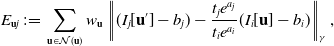
DSO extracts point candidates in the regions with enough gradient and regards one point as the intersection of the source pixel’s ray and the object. So only one parameter, that is, inverse depth, is used to represent the point. In the optimization process, residual pattern is used to enhance the differentiation of a single pixel, considering the trade off between computation and providing sufficient information. Several nearby pixels share the inverse depth of the middle pixel, which implies the fronto-parallel assumption that the surface of object is assumed to be parallel to the camera. Obviously, this assumption is just an approximation in the real world, which may fail to hold slanted surfaces, as Fig. 1 shows.
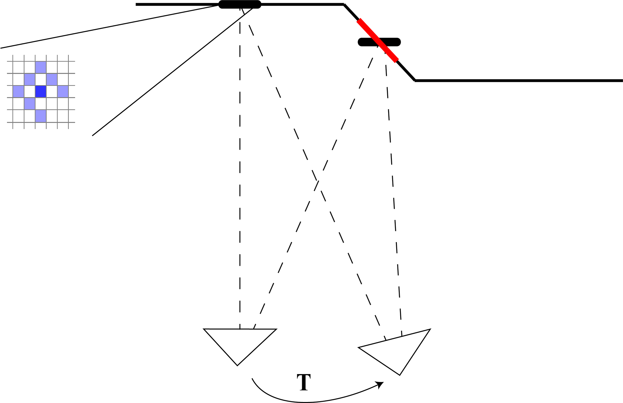
Figure 1. Approxiamtation error using a residual pattern in different situations. We can find that there is a certain deviation between the actual depth (bold red line) and the approximation (bold black line). The two triangles represent the camera poses at different times.
As the inverse depth only tells us where the point is, information about the orientation is not included. Therefore, the approximation error is unenviable in a point-based odometry. Instead, if the normal vector of the surface is known, the deviation can be reduced to zero theoretically. By providing useful information about the normal vectors of all detected planes, the final energy function is much easier to converge, especially in structured environments where large numbers of planar patches can be found.
4.2. Plane parameterization
The most intuitive representation of plane is Hesse notation, that is,
 \begin{equation} \textbf{n}_0^T \textbf{p}-d=0, \end{equation}
where
 $\textbf{n}_0$
represents the unit normal vector of the plane and
$\textbf{n}_0$
represents the unit normal vector of the plane and
 $d$
is the distance from the camera to the plane.
$d$
is the distance from the camera to the plane.
The parameterization
 $[\textbf{n}_0,d]$
is not a minimal representation, which has four variables while the DoF of plane is just three. Similar to [Reference Kaess20], we remove one DoF by forcing the distance term to 1:
$[\textbf{n}_0,d]$
is not a minimal representation, which has four variables while the DoF of plane is just three. Similar to [Reference Kaess20], we remove one DoF by forcing the distance term to 1:
 \begin{equation} \textbf{n}^T \textbf{p} -1=0, \end{equation}
where the plane parameterization
 $\textbf{n}=\textbf{n}_0/d$
becomes a minimal representation. Note that when
$\textbf{n}=\textbf{n}_0/d$
becomes a minimal representation. Note that when
 $d=0$
, there is also singularity. To avoid this, we will not build a global planar model similar to ref. [Reference Ma, Kerl, Stückler and Cremers8]. Instead, we only represent a plane in the camera coordinate. A plane with
$d=0$
, there is also singularity. To avoid this, we will not build a global planar model similar to ref. [Reference Ma, Kerl, Stückler and Cremers8]. Instead, we only represent a plane in the camera coordinate. A plane with
 $d$
approximating zero in the camera coordinates indicates that the plane passes through the camera center, which means it will be projected as a line (i.e., not detected as a plane). The plane will not be observed, thus avoiding from being added into the final optimization process. Local planar patches may not provide long-time consistent constraints as those of global planar models, but have much higher flexibility and adaptability.
$d$
approximating zero in the camera coordinates indicates that the plane passes through the camera center, which means it will be projected as a line (i.e., not detected as a plane). The plane will not be observed, thus avoiding from being added into the final optimization process. Local planar patches may not provide long-time consistent constraints as those of global planar models, but have much higher flexibility and adaptability.
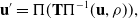
The geometric meaning of this parameterization is also clear: the norm of
 $\textbf{n}$
is the inverse distance from the origin point to the plane, while its direction represents the normal. So
$\textbf{n}$
is the inverse distance from the origin point to the plane, while its direction represents the normal. So
 $\textbf{n}$
is also called as inverse normal in this paper, which is illustrated in Fig. 2.
$\textbf{n}$
is also called as inverse normal in this paper, which is illustrated in Fig. 2.
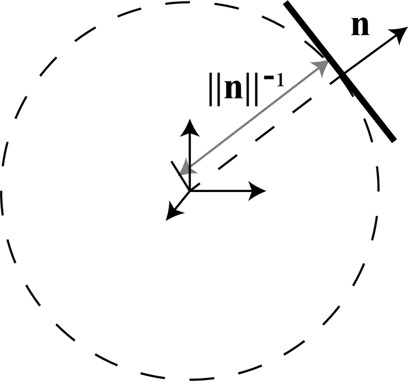
Figure 2. Illustration of inverse normal.
From the pinhole imaging model,
 \begin{equation} \textbf{p}=\rho ^{-1}\textbf{K}^{-1}\textbf{u}, \end{equation}
and Eq. (4), we can get the relation between inverse depth and inverse normal:
 \begin{equation} \rho = (\textbf{K}^{-1}\textbf{u})^T\textbf{n}, \end{equation}
We use
 $\textbf{p}=\Lambda (\textbf{u},\textbf{n})$
to represent this transformation.
$\textbf{p}=\Lambda (\textbf{u},\textbf{n})$
to represent this transformation.
The partial derivative of the inverse depth about the inverse normal can also be derived easily:
 \begin{equation} \frac{\partial \rho }{\partial \textbf{n}}=(\textbf{K}^{-1}\textbf{u})^T. \end{equation}
Then, we can get the Jacobin matrix about inverse normal through the chain rule
 $\frac{\partial f}{\partial \textbf{n}}=\frac{\partial f}{\partial \rho }\frac{\partial \rho }{\partial \textbf{n}}$
directly, based on the existing Jacobin matrix from DSO. Here,
$\frac{\partial f}{\partial \textbf{n}}=\frac{\partial f}{\partial \rho }\frac{\partial \rho }{\partial \textbf{n}}$
directly, based on the existing Jacobin matrix from DSO. Here,
 $f$
is the residual of all observations.
$f$
is the residual of all observations.
4.3. Model
We formulate the whole optimization problem with planes in this section, which is illustrated in Fig. 3. Compared to DSO, our point-plane system add additional planar constraints into the optimization.
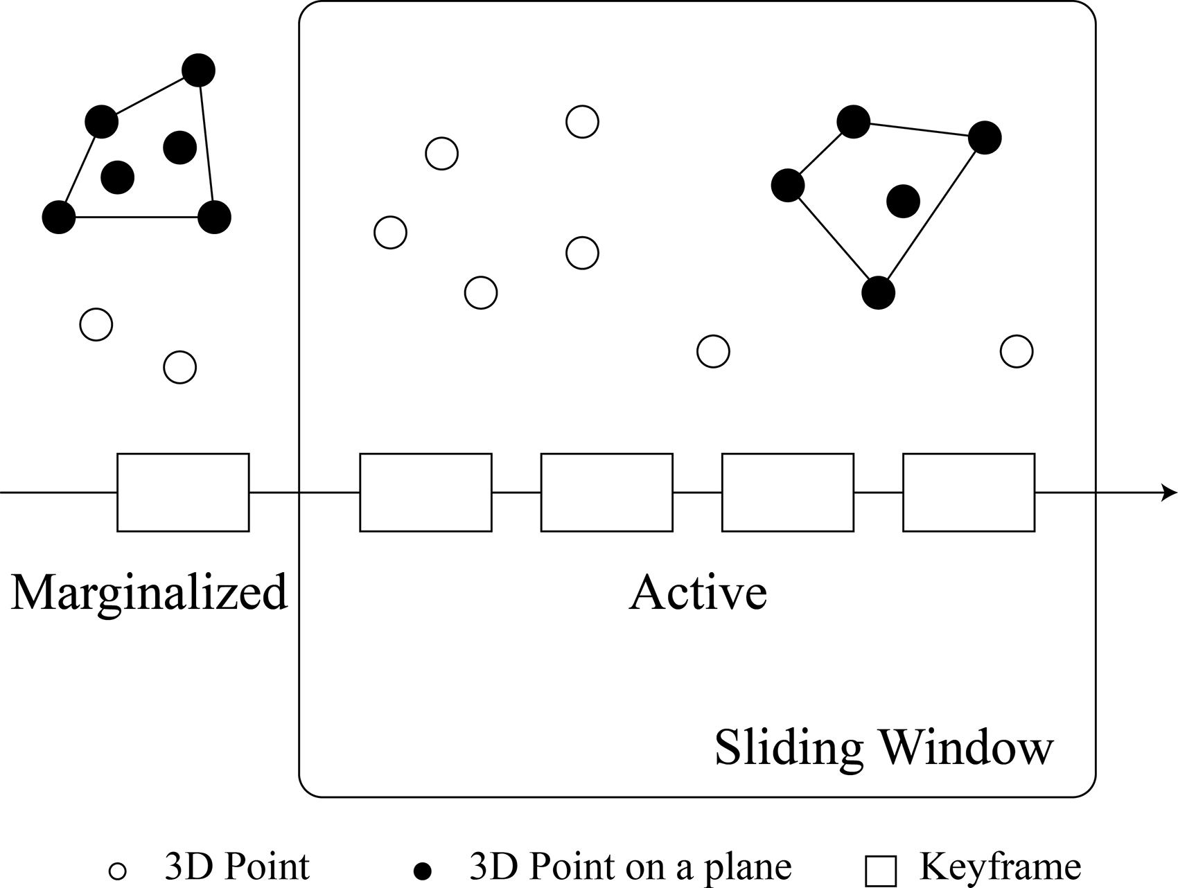
Figure 3. Illustration of inverse normal.
Suppose that we have got some planar patches in the local window with a set of keyframes
 $\mathcal{F}$
, the full target function is given by
$\mathcal{F}$
, the full target function is given by
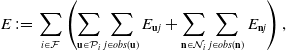 \begin{equation} E\,{:\!=}\,\sum _{i\in \mathcal{F}}\left(\sum _{\textbf{u} \in \mathcal{P}_i}\sum _{j\in obs(\textbf{u})}E_{\textbf{u}j}+\sum _{\textbf{n} \in \mathcal{N} _i}\sum _{j\in obs(\textbf{n})}E_{\textbf{n}j}\right), \end{equation}
where
 $\mathcal{P}_i$
represents all points in the
$\mathcal{P}_i$
represents all points in the
 $i$
th keyframe except those in the planar regions,
$i$
th keyframe except those in the planar regions,
 $\mathcal{N}_i$
is the set of all available planes,
$\mathcal{N}_i$
is the set of all available planes,
 $obs(\textbf{x})$
returns all observations of target
$obs(\textbf{x})$
returns all observations of target
 $\textbf{x}$
over all frames in the window, and
$\textbf{x}$
over all frames in the window, and
 $E_{\textbf{n}j}$
defines the cost energy of a planar patch
$E_{\textbf{n}j}$
defines the cost energy of a planar patch
 $\textbf{n}$
observed from another view
$\textbf{n}$
observed from another view
 $j$
, that is,
$j$
, that is,
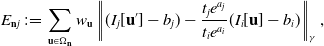 \begin{equation} E_{\textbf{n}j}\,{:\!=}\,\sum _{\textbf{u}\in \Omega _{\textbf{n}}}w_{\textbf{u}}\left\|(I_j[\textbf{u}']-b_j)-\frac{t_je^{a_j}}{t_ie^{a_i}}(I_i[\textbf{u}]-b_i)\right\|_{\gamma }, \end{equation}
 \begin{align} \textbf{u}'=\Pi (\textbf{T}\Lambda (\textbf{u}, \textbf{n})), \end{align}
where
 $\Omega _{\textbf{n}}$
is a region regarded as a plane, the extraction of which is discussed in next sections.
$\Omega _{\textbf{n}}$
is a region regarded as a plane, the extraction of which is discussed in next sections.
From Eqs. (8)--(9), we can find that only photometric residuals are used in our model. Geometric residuals are not adopted here. This is because that as we extract planar information from a monocular sparse odometry, the contours of planes are not clear; that is, it is difficult to judge if a projection pixel belongs to the plane. What’s more, the normal vectors are not as reliable as that from dense sensors. Inaccurate geometric constraints may destroy the stability of the system. Instead, photometric errors accumulated from single points are more flexible. A sudden increase of errors will be considered as a outlier or in bad conditions like being obscured and then be omitted in this time.
Another advantage is that no planar data association is needed in this way. Planar features are not distinguished as those of points. Some works like refs. [Reference Salas-Moreno, Glocken, Kelly and Davison7] and [Reference Hsiao, Westman, Zhang and Kaess9] used exhaustive searches over all candidates using intuitive metrics like the differences of normal vectors and distances, overlaps, and projection errors. However, these intuitive metrics are not appropriate for our small planar patches. With a direct photometric optimization, we avoid from finding tedious data association among planar patches.
The factor graph of the whole model is shown in Fig. 4. We can find that with the help of inverse normal, large numbers of variables about inverse depth can be reduced to only one variable, inverse normal, thus simplifying the graph. For example, without
 $\textbf{n}_1$
, there are hundreds of inverse depth
$\textbf{n}_1$
, there are hundreds of inverse depth
 $\rho$
that should be added into the factor graph. The simplification utilizes the important prior information, that is, points in a same plane shares common parameters. Therefore, the number of final variables to be optimized is significantly less than that of DSO.
$\rho$
that should be added into the factor graph. The simplification utilizes the important prior information, that is, points in a same plane shares common parameters. Therefore, the number of final variables to be optimized is significantly less than that of DSO.
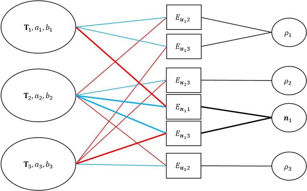
Figure 4. Factor graph of the point-plane odometry model. Here we show three keyframes with three points and one plane. Each factor term depends on the host frame (blue), target frame (red), and the point’s inverse depth or the plane’s inverse normal (black). The lines about planes are all bold.
4.4. Optimization
The Gauss-Newton method is applied to optimize all variables in the sliding window. The variable
 $\textbf{x}$
to be optimized consists of the increments of the camera intrinsic parameters
$\textbf{x}$
to be optimized consists of the increments of the camera intrinsic parameters
 $\textbf{c}$
, camera poses
$\textbf{c}$
, camera poses
 $\textbf{T}$
, light affine parameters
$\textbf{T}$
, light affine parameters
 $a,b$
, inverse depth
$a,b$
, inverse depth
 $\rho$
of all active points, and inverse normals
$\rho$
of all active points, and inverse normals
 $\textbf{n}$
of all active planes. Suppose that there are
$\textbf{n}$
of all active planes. Suppose that there are
 $k$
frames,
$k$
frames,
 $l$
points, and
$l$
points, and
 $m$
planes in the current window. Then the state variable
$m$
planes in the current window. Then the state variable
 \begin{equation} \textbf{x}=\bigg[\underbrace{\delta \textbf{c}^T, (\boldsymbol\xi _1^T,\delta a_1,\delta b_1),\cdots,(\boldsymbol\xi _k^T,\delta a_k,\delta b_k)}_{\textbf{x}_\alpha }, \underbrace{\delta \rho _1,\cdots,\delta \rho _l,\delta \textbf{n}_1^T,\cdots,\delta \textbf{n}_m^T}_{\textbf{x}_\beta }\bigg]^T, \end{equation}
can be computed through the linear equation
 \begin{equation} \textbf{J}^T\textbf{W} \textbf{J}\textbf{x}=-\textbf{J}^T\textbf{W}\textbf{r}, \end{equation}
where
 $\textbf{J}$
is the Jacobin matrix of the photometric residual
$\textbf{J}$
is the Jacobin matrix of the photometric residual
 $\textbf{r}$
about the variable
$\textbf{r}$
about the variable
 $\textbf{x}$
, and
$\textbf{x}$
, and
 $\textbf{W}$
is the weight matrix set intuitively. By using the Schur complement, the part
$\textbf{W}$
is the weight matrix set intuitively. By using the Schur complement, the part
 $\textbf{x}_{\alpha }$
can be derived firstly and then be used to compute
$\textbf{x}_{\alpha }$
can be derived firstly and then be used to compute
 $\delta \rho$
and
$\delta \rho$
and
 $\delta \textbf{n}$
, respectively. Though the dimension of
$\delta \textbf{n}$
, respectively. Though the dimension of
 $\textbf{x}_\beta$
is much larger than that of
$\textbf{x}_\beta$
is much larger than that of
 $\textbf{x}_\alpha$
, the computation is fast due to the sparsity of the Hessian matrix. What’s more, the adoption of inverse normal further reduces the dimension of
$\textbf{x}_\alpha$
, the computation is fast due to the sparsity of the Hessian matrix. What’s more, the adoption of inverse normal further reduces the dimension of
 $\textbf{x}_\beta$
. One important thing to note is that each plane patch must include enough active points to avoid from rank-deficient information matrix.
$\textbf{x}_\beta$
. One important thing to note is that each plane patch must include enough active points to avoid from rank-deficient information matrix.
The marginalization of planes follows the strategy of that of points. One difference is that the planes stay longer, as the projections of planar residuals cover a much larger area.
5. Grid-Based Plane Detection
In this section, we propose an effective plane detection algorithm for sparse monocular odometry, which is shown in Fig. 5. As mentioned before, it is impracticable to extract accurate planes with clear boundaries without dense depth map. Therefore, we just try to cluster points belonging to the same plane and generate plane patches simply consisting of sparse points. As a result, the detected planes may not be real actually, that is, a virtual plane consisting of real points can also be detected. But it does not influence the process of optimization.
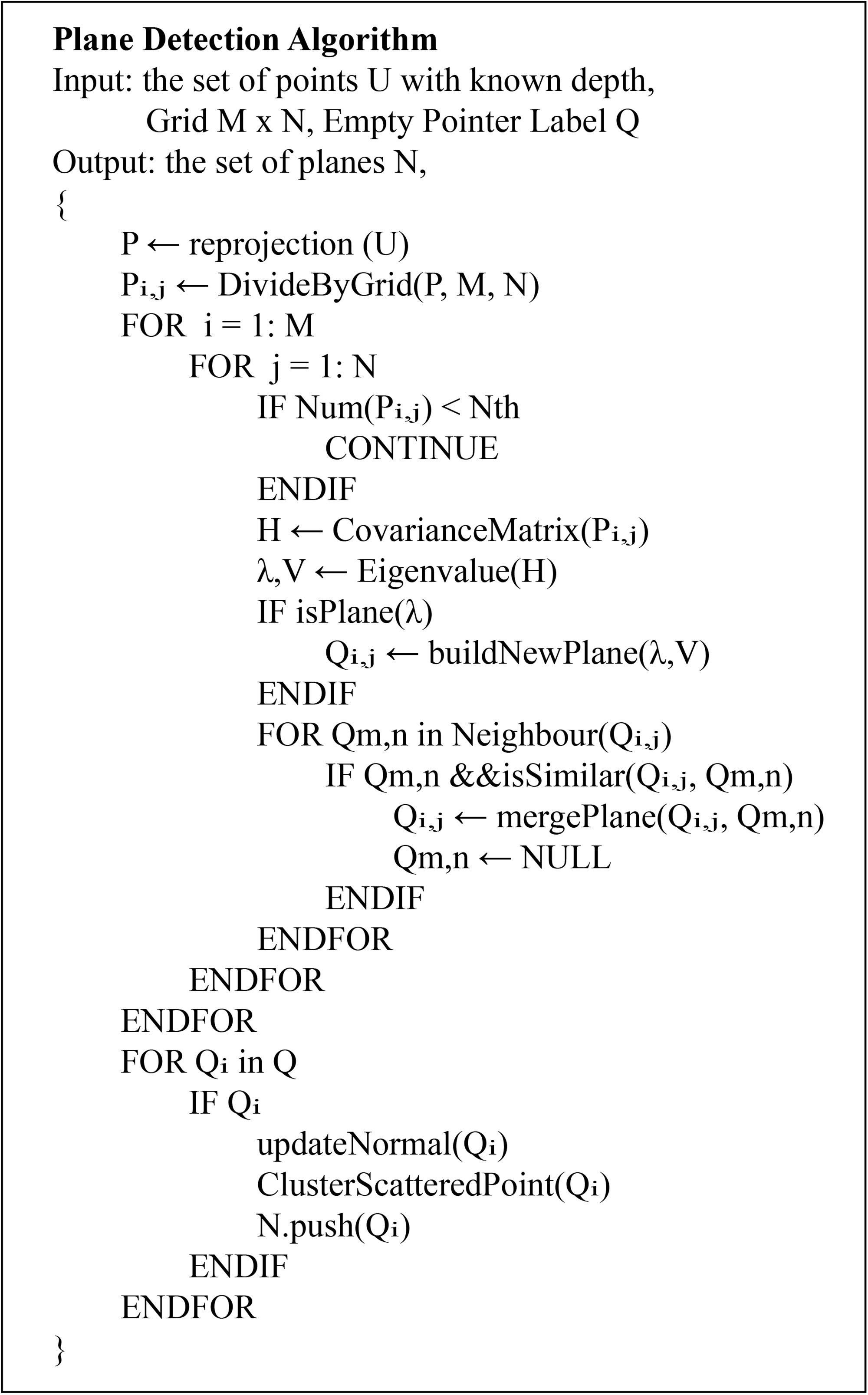
Figure 5. Grid-based plane detection algorithm.
DSO extracts immature points for each frame when added into the set of keyframes in the sliding window and activates them the next time a keyframe is built. Our process of plane detection starts when immature points in a keyframe are activated at the first time. From Fig. 5, we can see that a
 $M \times N$
grid is used to divide all points at first. The idea comes from [Reference Xiao, Zhang, Zhang, Zhang and Hildre15], that for a structured environment, if the points are divided into small grids, most of them should be in a planar region. So, our target is to find such planar regions through the grids. A
$M \times N$
grid is used to divide all points at first. The idea comes from [Reference Xiao, Zhang, Zhang, Zhang and Hildre15], that for a structured environment, if the points are divided into small grids, most of them should be in a planar region. So, our target is to find such planar regions through the grids. A
 $3 \times 3$
patch with six or less valid points will probably cause a problem to the plane detection criteria, and testing whether such patches are degenerated will increase the computational complexity [Reference Xiao, Zhang, Zhang, Zhang and Hildre15]. To guarantee rich information and avoid from high computational complexity, we only detect grids with enough points. We also set a relatively strict criteria of the plane features we use, including planar region judgment and plane merging, as is described in the following algorithm.
$3 \times 3$
patch with six or less valid points will probably cause a problem to the plane detection criteria, and testing whether such patches are degenerated will increase the computational complexity [Reference Xiao, Zhang, Zhang, Zhang and Hildre15]. To guarantee rich information and avoid from high computational complexity, we only detect grids with enough points. We also set a relatively strict criteria of the plane features we use, including planar region judgment and plane merging, as is described in the following algorithm.
The covariance matrices of points in each grid are computed, which are used to get eigenvalues and eigenvectors. As is known to all, the eigenvalues describe the distribution of a point cloud. Suppose the eigenvalues of a covariance matrix are sorted in ascending, that is,
 $\lambda _1<\lambda _2<\lambda _3$
, with corresponding eigenvectors
$\lambda _1<\lambda _2<\lambda _3$
, with corresponding eigenvectors
 $\textbf{v}_1,\textbf{v}_2,\textbf{v}_3$
. For a plane,
$\textbf{v}_1,\textbf{v}_2,\textbf{v}_3$
. For a plane,
 $\lambda _1$
must be a small quantity, while for a line, both
$\lambda _1$
must be a small quantity, while for a line, both
 $\lambda _1$
and
$\lambda _1$
and
 $\lambda _2$
are small quantities. So, we judge a plane by checking if
$\lambda _2$
are small quantities. So, we judge a plane by checking if
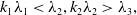 \begin{equation} k_1\lambda _1 < \lambda _2,k_2\lambda _2 > \lambda _3, \end{equation}
both hold at the same time, where
 $k_1,k_2$
are two constants, set as 1000 and 10 respectively in this paper.
$k_1,k_2$
are two constants, set as 1000 and 10 respectively in this paper.
After a new plane patch is built, we will try to merge it with nearby patches if exist. As we check all grids from top left to bottom right, we only test left and upper grids. Then, two planes are merged if their inverse normal are close, that is, the cosine value
 $cos<\textbf{n}_1,\textbf{n}_2>$
is larger than a threshold (0.99 here) and the distance between two patches
$cos<\textbf{n}_1,\textbf{n}_2>$
is larger than a threshold (0.99 here) and the distance between two patches
 $|||\textbf{n}_1||^{-1}-||\textbf{n}_2||^{-1}|$
is smaller than a threshold (0.01 here). After the process, we update the inverse normal for all merged planes and then try to cluster scattered points. To avoid from bringing too many outliers, we only test grids next to the planar regions. The criterion depends on the distance from the point to the plane. Two examples are illustrated in Fig. 6. We can find that points detected really belong to planes. Normally about 0 to 4 planes can be detected though this way in a keyframe, based on the density and quality of points. As is shown in Fig 6, some grids with apparent planar regions are not detected as our planar features. When no plane is detected, our SPPO degenerates to DSO and it is acceptable.
$|||\textbf{n}_1||^{-1}-||\textbf{n}_2||^{-1}|$
is smaller than a threshold (0.01 here). After the process, we update the inverse normal for all merged planes and then try to cluster scattered points. To avoid from bringing too many outliers, we only test grids next to the planar regions. The criterion depends on the distance from the point to the plane. Two examples are illustrated in Fig. 6. We can find that points detected really belong to planes. Normally about 0 to 4 planes can be detected though this way in a keyframe, based on the density and quality of points. As is shown in Fig 6, some grids with apparent planar regions are not detected as our planar features. When no plane is detected, our SPPO degenerates to DSO and it is acceptable.
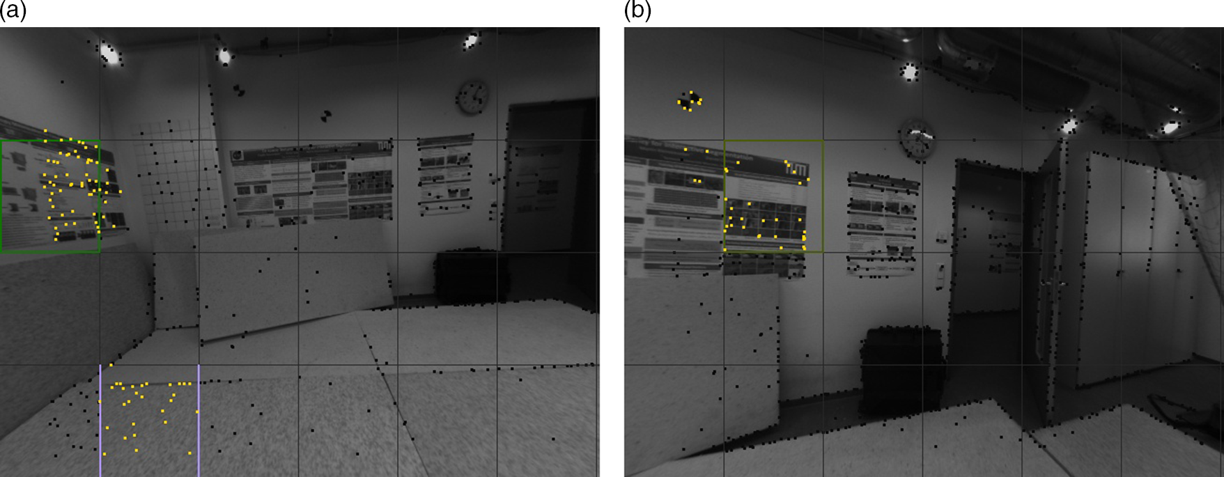
Figure 6. Two examples of plane detection from sparse points. Black points represent candidate points in the current frame (inverse depth is known) and gold points represent those detected belonging to planar regions. The black grids are set to divide all points while grids with other colors are the final remaining grids.
6. Experimental Results
In this section, we will illustrate the results of the proposed SPPO in different scenes and compare them with those of DSO. We use the default parameters of DSO, and the common ones are also not changed in SPPO. Some distinctive parameters in SPPO have been shown when they were firstly introduced. For most of them, the experimental results are insensitive, as long as they are not too singular. More details about the parameter settings can be referred to our open-source code: https://github.com/kidlin/sppo. All experiments run on a 3.7 GHz Intel machine with 16 GB memories. When comparing running times, the two methods run one by one to ensure that each project has sufficient CPU resources.
We use the TUM monoVO dataset [Reference Engel, Usenko and Cremers24] to evaluate our method, which consists of 50 photometrically calibrated sequences, including both indoor and outdoor scenes. Therefore, a lot of structured environments can be found here, although some natural scenes like grassland and forest also exist. As only loop-closure ground truth are provided, we use the alignment error
 $e_{align}$
[Reference Engel, Usenko and Cremers24] to evaluate the methods, that is,
$e_{align}$
[Reference Engel, Usenko and Cremers24] to evaluate the methods, that is,
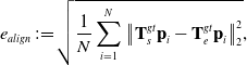 \begin{equation} e_{align}\,{:\!=}\,\sqrt{\frac{1}{N}\sum ^N_{i=1}\left\|\textbf{T}_s^{gt}\textbf{p}_i-\textbf{T}_e^{gt}\textbf{p}_i\right\|_2^2}, \end{equation}
where
 $N$
is the number of all available poses,
$N$
is the number of all available poses,
 $\textbf{p}$
is the translational part of the pose, and two relative transformations
$\textbf{p}$
is the translational part of the pose, and two relative transformations
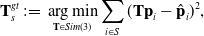 \begin{equation} \textbf{T}_s^{gt}\,{:\!=}\,\mathop{\arg \min }_{\textbf{T} \in Sim(3)} \sum _{i\in S}(\textbf{T}\textbf{p}_i-\hat{\textbf{p}}_i)^2, \end{equation}
 \begin{equation} \textbf{T}_e^{gt}\,{:\!=}\,\mathop{\arg \min }_{\textbf{T} \in Sim(3)} \sum _{i\in E}(\textbf{T}\textbf{p}_i-\hat{\textbf{p}}_i)^2, \end{equation}
where
 $S$
and
$S$
and
 $E$
are the sets of associated poses in the start segments and end segments respectively.
$E$
are the sets of associated poses in the start segments and end segments respectively.
6.1. Quantitative comparison
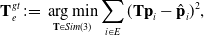
Figure 7(a) illustrates the alignment errors for both DSO and SPPO on the full TUM monoVO dataset. Generally speaking, the error distributions of the two are similar, while SPPO seems a little more robust on some sequences. This is clearer in Fig. 7(b), where we show the median values of each runs. From Fig. 7(b) we can find that in some scenes like Sequence 36, our SPPO performs much better. This is due to the fact that our approach utilizes more priori knowledge, that is, planar constraints in a small region, to help the optimization of the system. However, we can also find that in some sequences our approach does not even perform as well as DSO, which is due to the fact that natural environments are also included in some sequences.
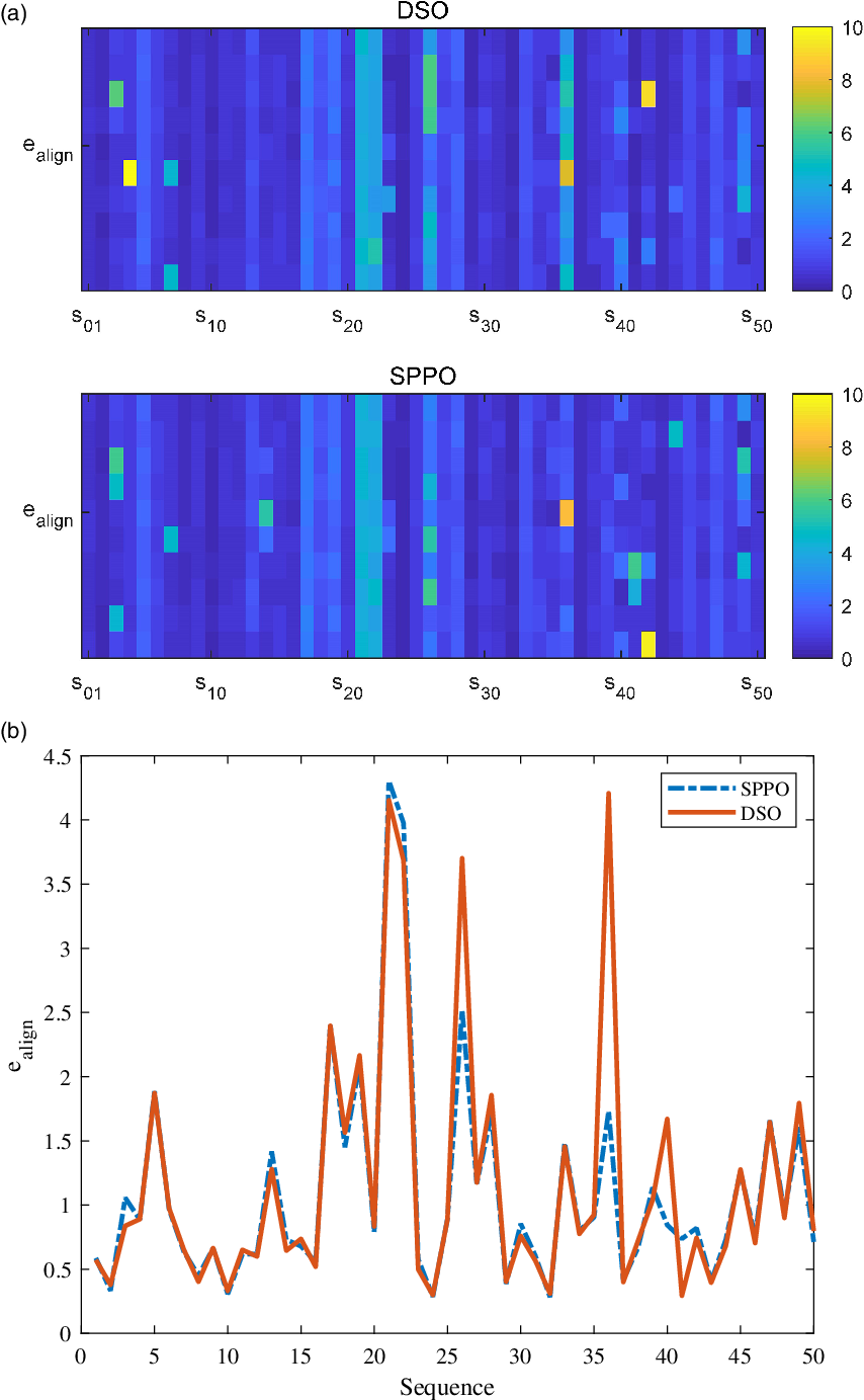
Figure 7. Results of the full TUM monoVO dataset. (a) Colorbar representation of all runs. Each sequence is implemented 10 times for both DSO and SPPO, which corresponds to the horizontal axis. And the vertical axis shows the index of sequences. (b) Median values of 10 runs for each run. The mean error of DSO is 1.274 while for SPPO it is 1.222.
Due to proper planar constraints, our SPPO runs faster than DSO, which is shown in Fig. 8. The mean running time of DSO is 33.2 ms while for SPPO, it is 25.3 ms. What’s more, in most sequences our approach is about 20% faster than DSO. The improvement is pretty important for some hardware-limited applications like mobile robots. The high efficiency mainly comes from three factors: (1) our efficient plane detection algorithm gives almost no pressure on the computing sources; (2) the introduction of planar constraints helps to reduce the size of the Hessian Matrix in the optimization, avoiding from unnecessary updates of points; (3) the planar constraints accelerates the convergence of the optimization.
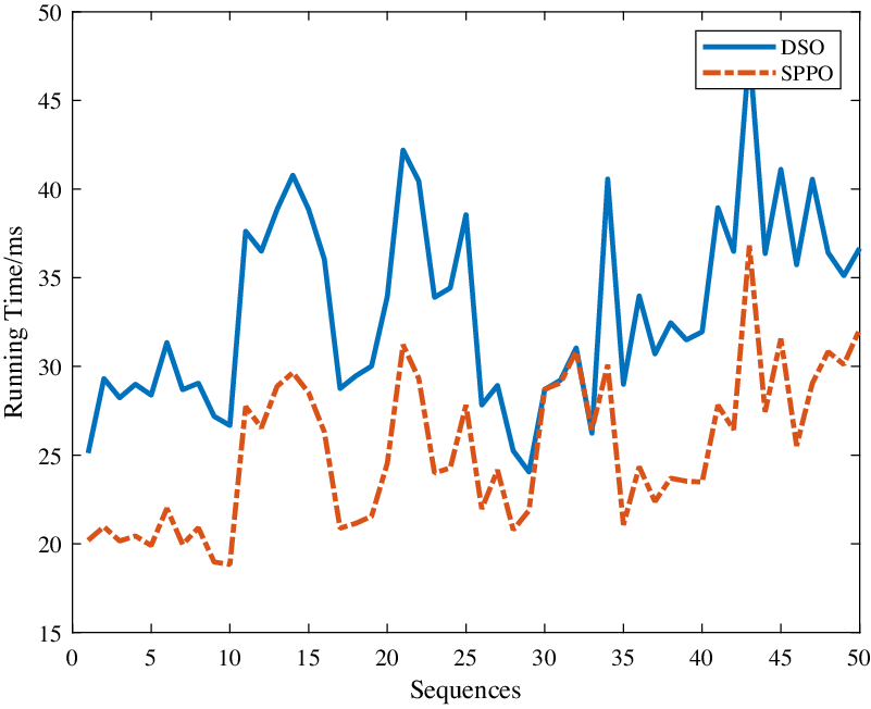
Figure 8. Running time of each sequences. We adopt the median value of 5 runs to avoid from stochastic factors. Here we do not force real-time for both two methods, and multi-threads are also opened. And the size of all rectified images is 640x480.
6.2. Discuss
Plane detection is a key step in the proposed point-plane odometry. Our grid-based plane detection algorithm performs well in most scenes, except some natural environments like lawn. The TUM monoVO dataset provides some outdoor scenes including lawn, forest, and so on. Fig. 9 shows four samples of plane detection in different scenes. In Fig. 9(a), two virtual planes are detected due to regular edge protrusions. And in Fig. 9(b), no planes are detected in a natural forest, which implies SPPO degenerates into DSO in fact. Fig. 9(c) shows some detected planes on the lawn while Fig. 9(d) illustrates a proper plane detected on a wall. In both Fig. 9(a) and (c), the detected planes are not stable, which implies that the additional planar constraints may give false optimization directions. This explains why our SPPO may perform a little worse than DSO in some sequences (see Fig. 7). Therefore, our SPPO is suggested to run in a structured environment, especially indoor scenes.
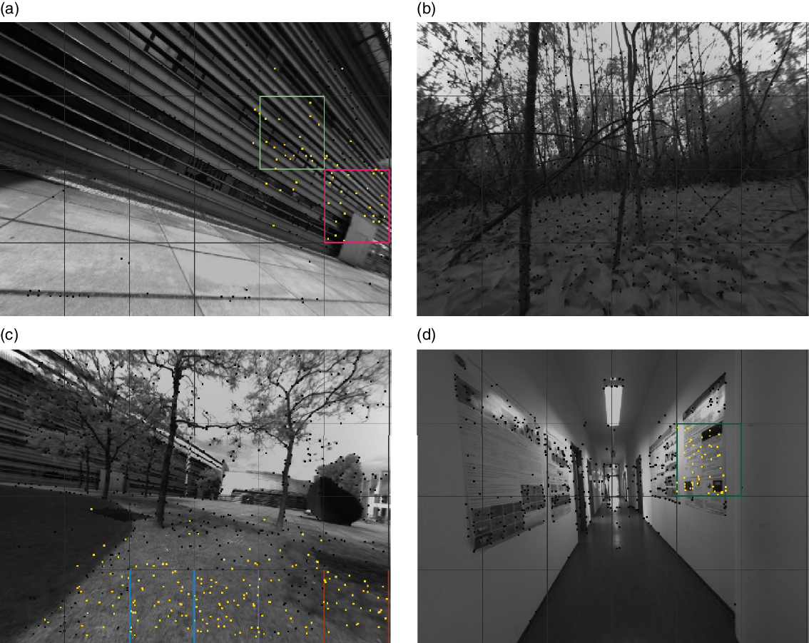
Figure 9. Four samples of plane detection. (a) A virtual plane; (b) No planes are detected in a natural forest; (c) False detections on the lawn; (d) A proper detection in structured environments.
When detecting planes, one important consideration is the factor between two eigen values, that is,
 $k_1,k_2$
in Eq. (12). The value of
$k_1,k_2$
in Eq. (12). The value of
 $k_1$
is used to find proper planes while the value of
$k_1$
is used to find proper planes while the value of
 $k_2$
is used to avoid from bad planes (clustered in a line). Figure 10 illustrates the accumulative alignment errors with different
$k_2$
is used to avoid from bad planes (clustered in a line). Figure 10 illustrates the accumulative alignment errors with different
 $k_1$
, from 100 to 10,000. We can find that the trends at the earlier stage are close to each other, which means they all work well in “good” environments. However, if
$k_1$
, from 100 to 10,000. We can find that the trends at the earlier stage are close to each other, which means they all work well in “good” environments. However, if
 $k_1=10,000$
, which implies less planes are added into the optimization, the errors grow much faster. Therefore, our point-plane joint optimization approach really helps to control the error growth in some situations.
$k_1=10,000$
, which implies less planes are added into the optimization, the errors grow much faster. Therefore, our point-plane joint optimization approach really helps to control the error growth in some situations.
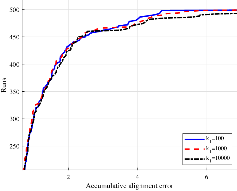
Figure 10. Accumulative alignment errors with different settings.
7. Conclusion
In this paper, we have proposed a SPPO in structured environments. We firstly introduce the limitations of points when a residual pattern is used in the optimization. Then, the concept of planes is introduced, which is parameterized using inverse normal. By introducing additional planar constraints, we build a SPPO framework based on DSO. Only photometric errors are used for planes, as the selected planes are just sparse, that is, full of holes. Then, we build the Hessian Matrix of plane by accumulating the information from the points that locate on it in the optimization. The marginalization strategy of planes is same as that of points. As for the plane detection, we propose an efficient grid-based detection algorithm, which is fast and adapt to the requirements of optimization. The proposed SPPO is evaluated on the TUM monoVO dataset. Compared to DSO, our method performs better in general and has a smaller running time due to the help of additional planar constraints. Further work will focus on how to add global planar constraints in the sparse odometry and how to utilize planar information to relocalize.


