


1. Introduction
Constant force mechanism (CFM) also known as quasi-zero stiffness mechanism, which can perform output a constant force in a certain range of input displacement [Reference Parlaktas1–Reference Javier, Daniel, Francisco and Jose3]. The CFM that can maintain the output force in a specific value has been widely adopted in application of ultraprecision polishing, micro-manipulation, and vibration isolation [Reference Zhang, Xiao, Zou and Xiao4–Reference Mammano and Dragoni6]. Generally speaking, the constant force can be realized by a closed-loop control method with force sensors and advanced algorithms. For instance, Choi et al. adopted a robust force tracking control to improve the performance of SMA-based flexible gripper [Reference Choi, Hua, Kim and Cheong7]. Huang et al. reported an automatic cell injection system based on force sensing and controlling method [Reference Huang, Sun, Su and Mills8]. Zhang et al. developed an automated robotic micromanipulation system with MEMS force sensor for studying the Drosophila larvae [Reference Zhang, Sobolevskl, Li, Rao and Liu9]. However, the aforementioned method required expensive sensors and complex algorithms which increases the cost of realizing constant force. To reduce the dependency on complicated control algorithms, CFMs consisting with passive elastic structure were presented from the perspective of mechanism design [Reference Li, Cheng and Xie10, Reference Todd, Jensen, Schultz and Hawkins11].
During the literature review, CFM can be realized by designing a specific curved-beam, shape optimization and stiffness combination methods. For curved-beam-based CFM, the constant force is generated by designing a special shape beam. Wang et al. developed a constant force bistable micro-mechanism with force regulation and overload protection functions [Reference Wang, Chen and Pham12]. Pedersen et al. designed a compliant mechanism that can deliver a constant output force to modify characteristics of the actuator by topology and size optimization methods [Reference Pedsresn, Fleck and Ananthasuresh13]. Similar to the curved-beam CFM, the shape optimization CFM generates a constant force output based on meticulously process. For example, Chen et al. presented a constant force clip to overcome snap-fit mating uncertainty relying on shape optimization of a cantilever-like structure [Reference Chen and Lan14]. Liu et al designed a compliant constant-force mechanism by topology and geometry optimization methods, which can generate a nearly constant output force over a range of input displacements [Reference Liu, Hsu, Chen and Chen15]. The difference between the curved beam and shape optimization CFM is that the former referring to fixed-guided beam and the latter based on fixed-free cantilever beam [Reference Meaders and Mattson16]. However, both of curved beam and shape optimization CFM are required to obtain the specific shape by analytical modeling which is a time-consuming process. Different with aforementioned two methods, stiffness-combination CFM obtains constant force by combination of PSS and negative-stiffness structure (NSS) [Reference Tian, Zhou, Wang, Lu, Yuan, Yang and Zhang17]. Ye et al. proposed a type of multistage CFM based on the parallel connection of negative and positive stiffness modules [Reference Ye, Ling, Kang, Feng and Xiao18]. Liu et al. designed a compliant constant force gripper by using the combination of positive stiffness and negative stiffness mechanism [Reference Liu, Zhang and Xu19]. Compared with curved beam and shape optimization CFMs, the stiffness combination CFM attracted wide attention for the advantages of simple structure, accurate output, and low requirement on materials.
However, in some applications, the changing of constant output force magnitude is desirable. For example, in applications that the initial desired force is unknown and in applications where a system calls for gradual change in output force over a range of motion [Reference Nahar and Sugar20]. Hence, to further expand the application of CFM, the design of variable constant force mechanism (VCFM) could be highly beneficial for these applications. Generally speaking, the variable constant force output can be realized by conventional rigid link mechanism and compliant mechanism. Due to the advantages of frictionless, no backlash, vacuum compatibility and compactness, a compliant VCFM is proposed in this study [Reference Chen and C.Lan21].
The main contribution of this paper is to propose a compliant VCFM with experimental verification. The remainder of this is organised as follows. Section 2 introduces the principle of VCFM realization based on the stiffness combination method. Section 3 presents the comparison of typical PSSs and NSSs, including the design of VCFM. Analytical modeling of positive and negative stiffness structure is established in Section 4. In addition, the sensitivity of structural parameters to constant force property is conducted in Section 5. Furthermore, experimental validation is presented in Section 6. Finally, conclusions are drawn in Section 7.
2. Principle of realization VCFM
To get a variable constant force, the output constant force should be obtained initially. In this paper, the constant force is obtained by combination of a PSS and NSS in parallel. The negative stiffness is generated by BSB with its buckling property, as shown in Fig. 1. Referring to this figure, as increasing the input displacement, the BSB will appear in two stable buckling positions, which correspond to Fig. 1(b) and (d), respectively. The first positive stiffness occurs at the interval (0,
 $x_1$
); the negative stiffness region locates in the interval (
$x_1$
); the negative stiffness region locates in the interval (
 $x_1$
,
$x_1$
,
 $x_3$
). When the displacement exceed
$x_3$
). When the displacement exceed
 $x_3$
, it begins to show the second positive stiffness characteristic, where
$x_3$
, it begins to show the second positive stiffness characteristic, where
 $x_2$
denotes a random point in the negative-stiffness interval (
$x_2$
denotes a random point in the negative-stiffness interval (
 $x_1$
,
$x_1$
,
 $x_3$
). To obtain a zero-stiffness characteristic, the magnitude of positive stiffness
$x_3$
). To obtain a zero-stiffness characteristic, the magnitude of positive stiffness
 $K_p$
and negative stiffness
$K_p$
and negative stiffness
 $K_n$
must be equal.
$K_n$
must be equal.

Figure 1. Force–displacement curve of BSB.
In the interval of (
 $x_1$
,
$x_1$
,
 $x_3$
), the output constant force
$x_3$
), the output constant force
 $F_{c1}$
can be derived referring to stiffness combination method:
$F_{c1}$
can be derived referring to stiffness combination method:
 \begin{equation} F_{c1} = (K_p + K_{b1})x_1 \end{equation}
where
 $K_{b1}$
denotes the value of first positive stiffness.
$K_{b1}$
denotes the value of first positive stiffness.
To realize variable constant output force, it means to regulate the magnitude of
 $F_{c1}$
with
$F_{c1}$
with
 $\Delta F_c$
, namely
$\Delta F_c$
, namely
 $F_{c1}\pm \Delta F_c$
. Referring to the Eq. (1), the force adjusting can be realized by two methods. One is to adjust the value of
$F_{c1}\pm \Delta F_c$
. Referring to the Eq. (1), the force adjusting can be realized by two methods. One is to adjust the value of
 $K_p + K_{b1}$
. However, the changing in stiffness involves massive workload and the difficulty to realize. The other method is to adjust the value of
$K_p + K_{b1}$
. However, the changing in stiffness involves massive workload and the difficulty to realize. The other method is to adjust the value of
 $x_1$
to the mechanism that is adopted in this paper.
$x_1$
to the mechanism that is adopted in this paper.
The principle of applying a preloading displacement to realize variable constant force output is depicted in Fig. 2, where the symmetric BSBs and a linear spring are connected in parallel [Reference Danh and Ahn22]. The end of the linear spring is connected to the preloading device to provide a preload force
 $F_r$
(or preload displacement
$F_r$
(or preload displacement
 $\Delta r$
) enabling the linear spring in pretightened condition. Simultaneously, the BSB will move upward when subjected to the preload force, but its deformation displacement is relatively small compared to the linear spring. Through applying prior preloading force, the output constant force can be regulated accordingly. In order to give a further explanation of this principle, force–displacement curve of the CFM in the different preloading conditions is shown in Fig. 3.
$\Delta r$
) enabling the linear spring in pretightened condition. Simultaneously, the BSB will move upward when subjected to the preload force, but its deformation displacement is relatively small compared to the linear spring. Through applying prior preloading force, the output constant force can be regulated accordingly. In order to give a further explanation of this principle, force–displacement curve of the CFM in the different preloading conditions is shown in Fig. 3.

Figure 2. The realization principle of VCFM.

Figure 3. Force–displacement curves of the VCFM in the different preloading conditions.
Referring to this figure, when a preload displacement
 $\pm \Delta r$
is applied, the positive-stiffness curve moves along
$\pm \Delta r$
is applied, the positive-stiffness curve moves along
 $x$
-axis in negative or positive direction with
$x$
-axis in negative or positive direction with
 $\Delta p$
, and a reaction force
$\Delta p$
, and a reaction force
 $K_p \Delta p$
generates accordingly. The force–displacement curve of the BSB moves along
$K_p \Delta p$
generates accordingly. The force–displacement curve of the BSB moves along
 $x$
-axis in positive or negative direction with
$x$
-axis in positive or negative direction with
 $\Delta b$
, and a reaction force
$\Delta b$
, and a reaction force
 $\mp K_{b1}\Delta b$
generates in the initial state. In accordance with
$\mp K_{b1}\Delta b$
generates in the initial state. In accordance with
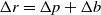 $\Delta r = \Delta p + \Delta b$
, the following equations can be obtained:
$\Delta r = \Delta p + \Delta b$
, the following equations can be obtained:
 \begin{equation} K_p \Delta p = K_{b1} \Delta b \end{equation}
 \begin{equation} F_{c2} = K_p (x_1 + \Delta r) + K_{b1}x_1 \end{equation}
 \begin{equation} F_{c3} = K_p (x_1 - \Delta r) + K_{b1}x_1 \end{equation}
where
 $F_{c2}$
and
$F_{c2}$
and
 $F_{c3}$
are the output constant force of the VCFM in
$F_{c3}$
are the output constant force of the VCFM in
 $\pm \Delta r$
preloading displacement. Particularly, the changing of constant force magnitude
$\pm \Delta r$
preloading displacement. Particularly, the changing of constant force magnitude
 $\Delta F_c$
is merely dependent on the applied preloading displacement on the linear spring. The actual numerical value of the changed constant force is the product of the positive stiffness and the preload displacement, namely
$\Delta F_c$
is merely dependent on the applied preloading displacement on the linear spring. The actual numerical value of the changed constant force is the product of the positive stiffness and the preload displacement, namely
 $K_p \Delta r$
. Meanwhile, the starting position of the constant force is directly related to the predeformation
$K_p \Delta r$
. Meanwhile, the starting position of the constant force is directly related to the predeformation
 $\Delta b$
of the BSB. According to Eq. (3), the following equations can be derived as
$\Delta b$
of the BSB. According to Eq. (3), the following equations can be derived as
 \begin{equation} \Delta r = \frac{F_{c2}-(K_p + K_{b1})x_1}{K_p} \end{equation}
 \begin{equation} \Delta b = \frac{K_p \Delta r}{K_p + K_{b1}} \end{equation}
Therefore, for a specific constant force, the required preload displacement can be derived by Eq. (5). Furthermore, through the given preloading displacement
 $+ \Delta r$
, the magnitude and the starting position of constant force can be deduced by Eqs. (3) and (6), respectively.
$+ \Delta r$
, the magnitude and the starting position of constant force can be deduced by Eqs. (3) and (6), respectively.
3. Design of VCFM
In this section, the designed VCFM is introduced including the comparison of some typical PSSs and BSBs.
3.1. Comparison of PSSs
As introduced in Section 2, the output force regulation can be realized by adjusting the preload displacement applied on the linear spring. For a specific CFM, the PSS denotes linear spring. Hence, choosing a suitable PSS is important for the realization of VCFM. Figure 4 presents the comparison of force–displacement curves of four typical PSSs via Workbench software. The straight beam exhibits highly nonlinear characteristics due to the stress stiffening. It is not suitable to act as a PSS because it cannot ideally neutralize the negative stiffness region of the bistable mechanism [Reference Ding, Zhao and Li23]. The folded beam exhibits good linear characteristics, but it is not suitable to apply preloading displacement in the input-displacement direction. The diamond-shape mechanism is similar to the U-shape mechanism in geometry shape. The difference is that the U-shape mechanism uses a flexible arc to connect flexible rods, and the diamond-shape mechanism uses a rigid rod. Considering the deformation of the flexible arc, the U-shape mechanism is more prone to fatigue failure [Reference Wong, Azid and Majlis24]. In addition, the analytical model for the U-shape is much complex than the diamond-shape mechanism. Therefore, the diamond-shape mechanism is chosen as a PSS for the designed VCFM.

Figure 4. Comparison of typical PSSs.
3.2. Comparison of BSBs
Generally speaking, the typical structural types of BSBs are V-shaped beam, cosine beam, and rigid-flexible hybrid beam, as shown in Fig. 5. The cosine beam exhibits better linearity in the negative stiffness stroke than other kind bistable beams. However, the complicated cosine shape beam requires exact prestressing that results it difficult to meet different work conditions [Reference Yan, Yu and Mehta25, Reference Han, Mller, Wallrabe and Korvink26]. V-shaped beam exhibits similar negative-stiffness characteristics to rigid-flexible hybrid beam [Reference Chen, Wu, Li and Wang27]. Owing to its advantages of simple structure and easy modeling, V-shaped beam is chosen as the NSS to utilize in the CFM design.

Figure 5. Comparison of typical BSBs.
3.3. Mechanical design
The 3D model of the designed VCFM is depicted in Fig. 6. The voice coil motor is utilized to provide driven force, and a force sensor is adopted to measure the reaction force. To adjust the preloading displacement directly and easily, the micrometer head is used as a preloaded device which is fixed on the base by a tightening nut. In addition, the base is mounted on the working stage through sliding grooves. Therefore, the assembly errors can be compensated by driving the micrometer head to move along
 $x$
direction linearity. The preloading displacement
$x$
direction linearity. The preloading displacement
 $\Delta r$
applied on the diamond- shape mechanism is realized by adjusting the micrometer head. The displacement
$\Delta r$
applied on the diamond- shape mechanism is realized by adjusting the micrometer head. The displacement
 $\Delta x$
at the end of the connector is generated by driven force
$\Delta x$
at the end of the connector is generated by driven force
 $F$
.
$F$
.

Figure 6. 3D model of the VCFM. 1-antivibration stage, 2-working stage, 3-micrometer head, 4-base, 5-tightening nut, 6-VCFM, 7-connector 1, 8-force sensor, 9-connector 2, 10-voice coil motor.
4. Analytical modeling
To obtain the force–displacement relationship of the designed VCFM, analytical model of the positive and negative stiffness structure is established in this section.
4.1. Modeling of PSS
As shown in Fig. 7(a), the diamond-shaped mechanism consists of four uniformed flexible beams and rigid rods. In this figure, where
 $L_1$
denotes length of the flexible beam,
$L_1$
denotes length of the flexible beam,
 $t_1$
represents width of the flexible beam,
$t_1$
represents width of the flexible beam,
 $\theta _1$
is angle between the flexible beam and the horizontal plane,
$\theta _1$
is angle between the flexible beam and the horizontal plane,
 $\Delta y_1$
is the output displacement, and
$\Delta y_1$
is the output displacement, and
 $F_1$
is the output force. The deformation of the diamond-shape mechanism can be calculated by superimposing the deformation of each section of the inclined flexible beam. When the deformation of one beam is studied, the other beams can be regarded as ideal rigid bodies. Considering the symmetric characteristic of the structure, the modeling of quarter diamond-shape mechanism is shown in Fig. 7(b).
$F_1$
is the output force. The deformation of the diamond-shape mechanism can be calculated by superimposing the deformation of each section of the inclined flexible beam. When the deformation of one beam is studied, the other beams can be regarded as ideal rigid bodies. Considering the symmetric characteristic of the structure, the modeling of quarter diamond-shape mechanism is shown in Fig. 7(b).

Figure 7. Modeling of diamond-shaped mechanism: (a) schematic diagram of mechanism deformation, (b) modeling of inclined cantilever beam.
Referring to Fig. 7(b), the following equation can be deduced as
 \begin{equation} 2(M_0 - M_1) = F_x L_1 sin \theta _1 - F_y L_1 cos \theta _1 \end{equation}
Furthermore, the following relationship can be obtained:
 \begin{equation} \frac{F_x(L_1 cos \theta _1)^2}{2EI} - \frac{M_1 L_1 cos \theta _1}{EI} = 0 \end{equation}
 \begin{equation} \frac{F_x(L_1 cos \theta _1)^3}{3EI} - \frac{M_1 (L_1 cos \theta _1)^2}{2EI} = \delta _{max} \end{equation}
where
 $\delta _{max}$
is the maximum deformation of the beam,
$\delta _{max}$
is the maximum deformation of the beam,
 $E$
is the Young’s modulus,
$E$
is the Young’s modulus,
 $I = b_1 t_1^3/ 12$
is the inertia moment, and
$I = b_1 t_1^3/ 12$
is the inertia moment, and
 $b_1$
is the out-plane width of the mechanism.
$b_1$
is the out-plane width of the mechanism.
 $\delta _{max}$
is composed of the deformation
$\delta _{max}$
is composed of the deformation
 $\delta _{bm}$
caused by the bending moment and the deformation
$\delta _{bm}$
caused by the bending moment and the deformation
 $\delta _s$
caused by the shear, namely:
$\delta _s$
caused by the shear, namely:
 \begin{equation} \delta _{max} = \delta _{bm} + \delta _{s} \end{equation}
According to Hook’s law
 $F=k \delta$
, the following equation can be derived:
$F=k \delta$
, the following equation can be derived:
 \begin{equation} \frac{1}{k_{max}} = \frac{1}{k_{bm}} + \frac{1}{k_{s}} \end{equation}
The maximum deflection due to bending moment can be expressed as
 \begin{equation} \delta _{bm}=\frac{F_1(L_1 cos \theta _1)^3}{12EI} \end{equation}
The deformation caused by the shear force can be written as
 \begin{equation} \delta _s = \frac{6(1+\mu )F_1 L_1 cos\theta _1}{5EA} \end{equation}
where
 $A = b_1 t_1$
is the cross-sectional area of the beam. According to Eq. (10), the maximum deformation can be derived as
$A = b_1 t_1$
is the cross-sectional area of the beam. According to Eq. (10), the maximum deformation can be derived as
 \begin{equation} \delta _{max} = \frac{F_1(L_1 cos \theta _1)^3}{12EI} + \frac{6(1+\mu )F_1 L_1 cos\theta _1}{5EA} \end{equation}
Therefore, the force–displacement expression of the diamond-shaped mechanism is
 \begin{equation} F_1 = \left(\frac{2(L_1 cos\theta _1)^3}{Eb_1 t_1^3} + \frac{12(1+\mu )F_1 L_1 cos\theta _1}{5Eb_1 t_1}\right)^{-1} \Delta x_1 \end{equation}
4.2. Modeling of BSB
As shown in Fig. 8, when applied an input displacement
 $\Delta x_2$
, the corresponding output force
$\Delta x_2$
, the corresponding output force
 $F_2$
is generated.
$F_2$
is generated.
 $L_2$
and
$L_2$
and
 $t_2$
are the length and width of the BSB, respectively, and
$t_2$
are the length and width of the BSB, respectively, and
 $\theta _2$
represents the inclination angle between the horizontal plane and the beam.
$\theta _2$
represents the inclination angle between the horizontal plane and the beam.

Figure 8. Modeling of BSB.
Referring to ref. [Reference Derakhshani, Momenzadeh and Berfifield28], the
 $j_{th}$
buckling force can be expressed as
$j_{th}$
buckling force can be expressed as
 \begin{equation} F_j = \frac{4EI_d \lambda _j^2}{l_j^2} \end{equation}
where
 $ I_d = b_2 t_2^3/ 12$
is the inertia moment, and
$ I_d = b_2 t_2^3/ 12$
is the inertia moment, and
 $l_j$
is the length at the
$l_j$
is the length at the
 $j_{th}$
critical segment,
$j_{th}$
critical segment,
 $\lambda _j$
=
$\lambda _j$
=
 $\pi, 4.493, 2\pi. . .$
,
$\pi, 4.493, 2\pi. . .$
,
 $j = 1, 2, 3. . .$
. The negative-stiffness expression of the BSB can be deduced as
$j = 1, 2, 3. . .$
. The negative-stiffness expression of the BSB can be deduced as
 \begin{equation} k_n \approx \frac{33EI_d}{L_2^3} \end{equation}
In accordance with Eqs. (11) and (12), the following equation can be deduced by
 \begin{equation} F_2 = ES\frac{\Delta x_2}{L_2}\left(\frac{\Delta x_2}{L_2} - sin \theta _2\right)\left(\frac{\Delta x_2}{L_2} - 2 sin \theta _2\right) \end{equation}
where
 $S = b_2 t_2$
is the cross-sectional area of the beam. From Eqs. (10) and (13), the fundamental force–displacement formula of the CFM in the nonpreloaded condition can be obtained:
$S = b_2 t_2$
is the cross-sectional area of the beam. From Eqs. (10) and (13), the fundamental force–displacement formula of the CFM in the nonpreloaded condition can be obtained:
 \begin{equation} F = \frac{E b_1 t_1^3 \Delta x}{2(L_1 cos \theta _1)^3} + ES\frac{\Delta x_2}{L_2}\left(\frac{\Delta x_2}{L_2} - sin \theta _2\right)\left(\frac{\Delta x_2}{L_2} - 2 sin \theta _2\right) \end{equation}
5. Sensitivity analysis
In general, the more flatness and larger stroke of constant-force output, the better the performance of CFM. To find an optimal solution of parameters, the analysis of structural parametric sensitivity of CFM is conducted.
To analyze the parametric sensitivity of constant-force performance, a series of force displacement curves, related to
 $L_1$
,
$L_1$
,
 $t_1$
,
$t_1$
,
 $\theta _2$
, and
$\theta _2$
, and
 $t_2$
, are depicted in Fig. 9. Referring to this figure, some conclusions can be summarized as follows: Firstly, the length of
$t_2$
, are depicted in Fig. 9. Referring to this figure, some conclusions can be summarized as follows: Firstly, the length of
 $L_1$
varies gradually from 22 to 28 mm with a 2 mm interval. The variation tendency of
$L_1$
varies gradually from 22 to 28 mm with a 2 mm interval. The variation tendency of
 $L_1$
is positively correlated to the travel range of the constant force, meaning that the larger the
$L_1$
is positively correlated to the travel range of the constant force, meaning that the larger the
 $L_1$
becomes, the longer the constant-force travel range. However, the amplitude of force is inversely proportional to
$L_1$
becomes, the longer the constant-force travel range. However, the amplitude of force is inversely proportional to
 $L_1$
. In addition, the smaller the
$L_1$
. In addition, the smaller the
 $L_1$
, the greater the influence of
$L_1$
, the greater the influence of
 $L_1$
exists on the force. Secondly,
$L_1$
exists on the force. Secondly,
 $t_1$
of the diamond-shaped mechanism increases from 1.2 to 1.8 mm with an interval of 0.2 mm. It is seen that the force increases as
$t_1$
of the diamond-shaped mechanism increases from 1.2 to 1.8 mm with an interval of 0.2 mm. It is seen that the force increases as
 $t_1$
increases. The relationship between the force and
$t_1$
increases. The relationship between the force and
 $t_1$
is approximately direct proportional. Thirdly,
$t_1$
is approximately direct proportional. Thirdly,
 $\theta _2$
of the bi-stable beam varies gradually from
$\theta _2$
of the bi-stable beam varies gradually from
 $6^\circ$
to
$6^\circ$
to
 $9^\circ$
with an interval of
$9^\circ$
with an interval of
 $1^\circ$
. It should be pointed that the constant-force travel range becomes larger and larger as
$1^\circ$
. It should be pointed that the constant-force travel range becomes larger and larger as
 $\theta _2$
is increasing. An increase of
$\theta _2$
is increasing. An increase of
 $1^\circ$
for
$1^\circ$
for
 $\theta$
leads to a force increase of approximately 2 N. Nonetheless, the relationship between the force and
$\theta$
leads to a force increase of approximately 2 N. Nonetheless, the relationship between the force and
 $\theta$
is not directly proportional. Finally,
$\theta$
is not directly proportional. Finally,
 $t_2$
of the bistable beam changes gradually from 0.6 to 1.2 mm with a 0.2 mm interval. These observations imply that
$t_2$
of the bistable beam changes gradually from 0.6 to 1.2 mm with a 0.2 mm interval. These observations imply that
 $t_2$
has no apparently significant connection with critical buckling positions and ranges, merely making a difference to values of stiffness. The most interesting phenomenon is that multiple force–displacement curves can always intersect at one point. As discussed previously, it can be concluded that
$t_2$
has no apparently significant connection with critical buckling positions and ranges, merely making a difference to values of stiffness. The most interesting phenomenon is that multiple force–displacement curves can always intersect at one point. As discussed previously, it can be concluded that
 $\theta _2$
of the bistable beam has the greatest influence on the constant-force performance.
$\theta _2$
of the bistable beam has the greatest influence on the constant-force performance.

Figure 9. Parametric sensitivity analysis of the CFM: (a)
 $L_1$
, (b)
$L_1$
, (b)
 $t_1$
, (c)
$t_1$
, (c)
 $\theta _2$
, (d)
$\theta _2$
, (d)
 $t_2$
.
$t_2$
.
6. Experimental verification
In this section, experimental setup is established to verify the reliability of designed physical configuration and the correctness of analytical analysis. The VCFM prototype is fabricated with high flexibility material PLA-ST, with its density
 $\rho=$
 $1250\, {\rm kg/m}^3$
, Young’s modulus
$1250\, {\rm kg/m}^3$
, Young’s modulus
 $E=1.477\,{\rm GPa}$
, and Poisson’s ratio
$E=1.477\,{\rm GPa}$
, and Poisson’s ratio
 $\mu=0.3$
. Referring to the FEA-based optimization method [Reference Ding, Li and Li29], the obtained optimal architectural parameters are shown in Table I.
$\mu=0.3$
. Referring to the FEA-based optimization method [Reference Ding, Li and Li29], the obtained optimal architectural parameters are shown in Table I.
Table I. Architectural parameters of the VCFM.

6.1. Experimental setup
As shown in Fig. 10, a VCFM prototype is fabricated with a 3D printer (model: 3DP-25-4F) to verify the designed concept. The voice coil motor (model: TMEC100-015-000) is driven by a commercial linear servo amplifier (model: ACJ-055-18) to deliver a nominal travel stroke of 10 mm. To measure the reaction force of the mechanism, a force sensor (model: DS2-XD) is mounted at the end of input. A grating ruler (model: LaRW1-3D, Fagor Automation) is integrated to measure the input displacement of voice coil motor. The preload displacement is adjusted by the micrometer head for exhibiting different force–displacement characteristics.

Figure 10. Experimental setup.
6.2. Experimental results
The comparison of force–displacement curves of obtained experimental data, theoretical and simulation results in non-preloading conditions are depicted in Fig. 11. Referring to this figure, all these curves are exhibiting constant-force property in some degree. The differs of obtained three curves can be explained by following three reasons. First, the size of the finite element meshing process is relatively rough due to the computer performance. Second, the material properties of final printed prototype may be different from the given theoretical values partially because of the printing method and the filling density. Finally, the variation of pretightening force on bolts for fastening VCFM could also lead to the deviation of constant force during the experimental process.

Figure 11. Comparison of force–displacement curves in non-preload condition.
Referring to the experimental data, the output force is ranging from 10.75 to 11.26 N in the interval of [Reference Wang, Zhao, Gao and Yang2, Reference Zhang, Xiao, Zou and Xiao4] mm with an approximate 11.15 N output constant force. The fluctuation value of constant force is 4.5% of the maximum value. Meanwhile, the fluctuation of the force is +0.11 and −0.4 N, which is +0.9% and −3.5% to the average constant force value 11.15 N. Therefore, it meets constant-force definition proposed in the literatures [Reference Hou and Lan30]. Furthermore, according to Table II, Eqs. (10) and (13), the positive-stiffness amplitude of the diamond-shaped mechanism
 $K_p$
is 1.4 N/mm, and the first positive-stiffness amplitude of the BSB
$K_p$
is 1.4 N/mm, and the first positive-stiffness amplitude of the BSB
 $K_{b1}$
is about 5.9 N/mm.
$K_{b1}$
is about 5.9 N/mm.
Table II. Comparison of analytical and experimental data.
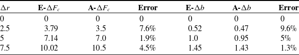
The process to validate the proposed concept is equivalent to verify the correctness of Eqs. (3) and (6). Considering the prototype dimensional size, stretchability, and the rebound limit of the material, the applied preload displacements are 0, 2.5, 5, and 7.5 mm, respectively, as shown in Fig. 12.

Figure 12. Pictures of different preloaded states.
The force–displacement data responsible for the proposed VCFM are collected in different preloading conditions. The changing of constant force and starting position is shown in Fig. 13 (a) and (b), respectively. When preloading displacement of 0, 2.5, 5, and 7.5 mm are applied, the corresponding constant force is 11.15, 14.94, 18.29, and 21.17 N. The constant force strokes are all close to 2 mm in different preloading conditions. Referring to Eqs. (3) and (6),
 $\Delta F_c$
and
$\Delta F_c$
and
 $\Delta b$
can be deduced as illustrated in Table II. The explanation for the error of experimental data
$\Delta b$
can be deduced as illustrated in Table II. The explanation for the error of experimental data
 $\Delta F_c$
and analytical data
$\Delta F_c$
and analytical data
 $\Delta _b$
is listed as follows. With the increasing of preloading displacement, the capability of elastic recovery of the mechanism is significantly reduced. In addition, the positive stiffness has changed after several times loading, while the theoretical analysis still believes that the positive stiffness remains constant. Moreover, the first positive stiffness of the BSB presents noninearity characteristic, whereas theoretical analysis regarded it as a constant value.
$\Delta _b$
is listed as follows. With the increasing of preloading displacement, the capability of elastic recovery of the mechanism is significantly reduced. In addition, the positive stiffness has changed after several times loading, while the theoretical analysis still believes that the positive stiffness remains constant. Moreover, the first positive stiffness of the BSB presents noninearity characteristic, whereas theoretical analysis regarded it as a constant value.

Figure 13. Experimental force–displacement curves in different preload displacements: (a) changing of constant-force; (b) changing of constant-force starting point.
7. Conclusions
This paper proposed a configuration type of VCFM referring to the stiffness combination principle. By adjusting the preload displacements on designed diamond-shaped compliant mechanism, the magnitude of output constant force can be easily changed. The mathematical model of PSS and NSS is established according to Hooke’s law. The analytical results indicated that the changing of constant force is only related to applied displacement on PSS, and the starting position of constant travel is associated with the predeformation of the BSB. Experimental studies are conducted on the prototype to further validate the correctness of the theoretical analysis. By comparing the experimental and analytical results of
 $\Delta F_c$
and
$\Delta F_c$
and
 $\Delta b$
in different preloading conditions, the errors are reasonable and acceptable which are all within 9.6%. The designed VCFM have a potential application in the field that requires force regulation to meet different working environments.
$\Delta b$
in different preloading conditions, the errors are reasonable and acceptable which are all within 9.6%. The designed VCFM have a potential application in the field that requires force regulation to meet different working environments.
Acknowledgements
Bingxiao Ding helped in conceiving the study concept and design, drafting and revising the manuscript, and obtaining funding. Xuan Li helped in acquiring the data, analyzing and interpreting the data, and drafting the manuscript. Yangmin Li helped in revising the manuscript, obtaining funding, and supervising the study. The authors would like to acknowledge Song Lu for his suggestions for improving the pictures quality. All authors have read and agreed to the published version of the manuscript.
Funding
This work is supported by Huxiang High Level Talent Project of Hunan Province (Grant No. 2019RS1066) and the Project State Key Laboratory of Ultra-precision Machining Technology of Hong Kong Polytechnic University (Project ID: BBXG).


