No-signaling Linear PCPs

Abstract

In this paper, we give a no-signaling linear probabilistically checkable proof (PCP) system for polynomial-time deterministic computation, i.e., a PCP system for ${\mathcal {P}}$ such that (1) the PCP oracle is a linear function and (2) the soundness holds against any (computational) no-signaling cheating prover, who is allowed to answer each query according to a distribution that depends on the entire query set in a certain way. To the best of our knowledge, our construction is the first PCP system that satisfies these two properties simultaneously.

As an application of our PCP system, we obtain a 2-message scheme for delegating computation by using a known transformation. Compared with existing 2-message delegation schemes based on standard cryptographic assumptions, our scheme requires preprocessing but has a simpler structure and makes use of different (possibly cheaper) standard cryptographic primitives, namely additive/multiplicative homomorphic encryption schemes.

1 Introduction

Linear PCP. Probabilistically checkable proofs, or PCPs, are proof systems with which one can probabilistically verify the correctness of statements with bounded soundness error by reading only a few bits of proof strings. A central result about PCPs are the PCP theorem [4, 5], which states that every $\mathcal {NP}$ statement has a PCP system such that the proof string is polynomially long and the verification requires only a constant number of bits of the proof string (the soundness error is a small constant and can be reduced by repetition).

An important application of PCPs to Cryptography is succinct argument systems, i.e., argument systems that have very small communication complexity and fast verification time. A famous example of such argument systems is that of Kilian [41], which proves an $\mathcal {NP}$ statement by using PCPs as follows.

• 1. The prover first generates a polynomially long PCP proof for the statement (this is possible thanks to the PCP theorem) and succinctly commits to it by using Merkle’s tree-hashing technique.

• 2. The verifier queries a few bits of the PCP proof just like the PCP verifier.

• 3. The prover reveals the queried bits by appropriately opening the commitment using the local opening property of Merkle’s tree-hashing.

This argument system of Kilian has communication complexity and verification time that depend on the classical $\mathcal {NP}$ verification time only logarithmically; that is, a proof for the membership of an instance x in an $\mathcal {NP}$ language L has communication complexity and verification time $\mathsf{poly}(\lambda + |x | + \log t)$, where $\lambda$ is the security parameter, t is the time to evaluate the $\mathcal {NP}$ relation of L on x, and $\mathsf{poly}$ is a polynomial that is independent of L. Kilian’s technique was later extended to obtain succinct non-interactive argument systems (SNARGs) for $\mathcal {NP}$ in the random oracle model [46] as well as in the standard model with non-falsifiable assumptions (such as the existence of extractable hash functions), e.g., [13, 28].¹

Recently, the studies of succinct argument systems have been boosted by the use of a specific type of PCPs called linear PCPs, which are PCPs such that the honest proofs are linear functions (i.e., the honest proof strings are the truth tables of linear functions).² (The proof strings of linear PCPs are exponentially long in general, but each bit of the proof strings can be computed efficiently by evaluating the underlying linear functions). A nice property of linear PCPs is that they often have much simpler structures than the polynomially long PCPs; as a result, the use of linear PCPs often lead to simpler constructions of succinct argument systems. The use of linear PCPs in the context of succinct argument systems was initiated by Ishai, Kushilevitz, and Ostrovsky [37], who used them for constructing an argument system for $\mathcal {NP}$ with a laconic prover (i.e., a prover that sends to the verifier only short messages). Subsequently, several works obtain practical implementations of the argument system of Ishai et al. [49,50,51,52,53], whereas others extended the technique of Ishai et al. for the use for SNARGs and obtained practical implementations of preprocessing SNARGs (i.e., SNARGs that require expensive (but reusable) preprocessing setups) [9, 11, 16].

No-signaling PCP. Very recently, Kalai, Raz, and Rothblum [39, 40] found that PCPs with a stronger soundness guarantee, called soundness against no-signaling provers, are useful for constructing 2-message succinct argument systems under standard assumptions. Concretely, Kalai et al. [39, 40] first constructed no-signaling PCPs (i.e., PCPs that are sound against no-signaling provers) for deterministic computation, and next showed that their no-signaling PCPs can be used to obtain 2-message succinct argument systems for deterministic computation under the assumptions of the existence of quasi-polynomially secure fully homomorphic encryption schemes or (2-message, polylogarithmic-communication, single-server) private information retrieval schemes. The succinct argument systems of Kalai et al. differ from prior ones in that they can handle only deterministic computation but require just two messages and is proven secure under standard assumptions. (In contrast, the argument system of Kilian and prior SNARG systems can handle non-deterministic computation but the former requires four messages and the latter are proven secure only in ideal models such as the random oracle model or under non-falsifiable knowledge-type assumptions).

As observed by Kalai et al. [39, 40], 2-message succinct argument systems have a direct application in delegating computation [32] (or verifiable computation [30]). Specifically, consider a setting where there exist a computationally weak client and a computationally powerful server, and the client wants to delegate a heavy computation to the server. Given a 2-message succinct argument system, the client can delegate the computation to the server in such a way that it can verify the correctness of the server’s computation very efficiently (i.e., much faster than doing the computation from scratch).

After the results of Kalai et al. [39, 40], no-signaling PCPs and their applications to delegation schemes have been extensively studied. Kalai and Paneth [38] extend the results of Kalai et al. [40] and obtain a delegation scheme for deterministic RAM computation, and Brakerski, Holmgren, and Kalai [20] further extend it so that the scheme is adaptively sound (i.e., sound even when the statement is chosen after the verifier’s message) and in addition can be based on polynomially hard standard cryptographic assumptions. Paneth and Rothblum [47] give an adaptively sound delegation scheme for deterministic RAM computation with public verifiability (i.e., with a property that not only the verifier but also anyone can verify proofs) albeit with the use of a new cryptographic assumption. Badrinarayanan, Kalai, Khurana, Sahai, and Wichs [7] give an adaptively sound delegation scheme for low-space non-deterministic computation (i.e., non-deterministic computation whose space complexity is much smaller than time complexity) under sub-exponentially hard cryptographic assumptions.

Kalai et al. [39, 40] and the abovementioned subsequent works on delegation schemes use no-signaling PCPs with polynomial length. As a result, compared with the delegation schemes that can be obtained from, e.g., the preprocessing SNARGs based on linear PCPs [9, 11, 16], their delegation schemes have complex structures.

1.1 Our Results

In this paper, we study the problem of constructing no-signaling linear PCPs, i.e., linear PCPs that are sound against no-signaling provers. Our main motivation is to obtain a PCP that inherits good properties from both of linear PCPs and no-signaling PCPs. Thus, our goal is to obtain a no-signaling linear PCP that can be used to obtain a 2-message delegation scheme that is secure under standard cryptographic assumptions (like those that are based on no-signaling PCPs) and has a simple structure (like those that are based on linear PCPs).

Main Result: No-signaling Linear PCP for $\varvec{{\mathcal {P}}}$ . The main result of this paper is an unconditional construction of no-signaling linear PCPs for polynomial-time deterministic computation. We focus our attention on PCPs that proves correctness of arithmetic circuit computation, so our construction handles statements of the form $(C, \varvec{x}, \varvec{y})$, where $C$ is a polynomial-size arithmetic circuit and the statement to be proven is “$C(\varvec{x}) = \varvec{y}$ holds.”

Theorem

(informal). There exists a no-signaling linear PCP for the correctness of polynomial-size arithmetic circuit computation. The proof generation algorithm runs in time $\mathsf{poly}(|C |)$, the verifier query algorithm runs in time $\mathsf{poly}(\lambda + |C |)$, and the verifier decision algorithm runs in time $\mathsf{poly}(\lambda + |\varvec{x} | + |\varvec{y} |)$.

A formal statement of this theorem is given as Theorem 1 in Sect. 4. To the best of our knowledge, our construction is the first linear PCP that is sound against no-signaling provers. (See Sect. 1.3 for concurrent independent works).

Our no-signaling linear PCP inherits simplicity from existing linear PCPs. Indeed, the proof string of our PCP is identical with that of the well-known linear PCP of Arora, Lund, Motwani, Sudan, and Szegedy [4]. Regarding the verifier, we added slight modifications to that of Arora et al. to simplify the analysis; however, we do not think that these modifications are fundamental.

The analysis of our PCP is, at a very high level, a combination of the analysis of the linear PCP of Arora et al. [4] and that of the no-signaling PCP of Kalai et al. [40]. A difficulty comes from the fact that the analysis of the no-signaling PCP of Kalai et al. partly rely on the specific construction of their PCP (which is based on the PCP of Babai, Fortnow, Levin, and Szegedy [6]), and we overcome this difficulty by modifying the analysis of the no-signaling PCP of Kalai et al. appropriately by borrowing techniques from the analysis of the linear PCP of Arora et al. Along the way, we also modify the analysis of Kalai et al. so that, unlike the analysis of Kalai et al., our analysis does not require that the statement is represented by an “augmented layered circuit” and only requires that it is represented by a layered circuit,³ so our PCP can work on smaller and simpler circuits; we think that this modification may be of independent interest. (The downside of this modification is that the analysis of no-signaling soundness becomes a little more complex. Specifically, we cannot use the notion of local-assignment generators [47] to analyze no-signaling soundness in a modular way). A more detailed overview of our analysis is given in Sect. 3.

Application: Delegation Scheme for $\varvec{{\mathcal {P}}}$ in the Preprocessing Model. As an application of our no-signaling linear PCP, we construct a 2-message delegation scheme for polynomial-time deterministic computation under standard cryptographic assumptions. Just like previous linear-PCP–based delegation schemes and succinct arguments (such as that of Bitansky et al. [16]), our delegation scheme works in the preprocessing model, so our scheme uses expensive offline setups that can be used for proving multiple statements. When the statement is $(C, \varvec{x}, \varvec{y})$, the running time of the client is $\mathsf{poly}(\lambda + |C |)$ in the offline phase and is $\mathsf{poly}(\lambda + |\varvec{x} | + |\varvec{y} |)$ in the online phase. Our delegation scheme is adaptively secure in the sense that the input $\varvec{x}$ can be chosen in the online phase, and is “designated-verifier type” in the sense that the verification requires a secret key. We obtain our delegation scheme by applying the transformation of Kalai et al. [39, 40] on our no-signaling liner PCP. (The transformation of Kalai et al., which is closely related to those of Biehl, Meyer, and Wetzel [12] and Aiello, Bhatt, Ostrovsky, and Rajagopalan [1], transforms a no-signaling PCP to a 2-message delegation scheme).

Compared with the existing 2-message delegation schemes based on polynomially long no-signaling PCPs (such as that of Kalai et al. [40]), our scheme requires preprocessing, but has a simple structure and uses different (possibly cheaper) tools thanks to the use of linear PCPs. Concretely, thanks to the use of linear PCPs, we can avoid the use of fully homomorphic encryption schemes or 2-message private information retrieval schemes, and can instead use additive homomorphic encryption schemes over prime-order fields (such as that of Goldwasser and Micali [33]) or multiplicative homomorphic encryption schemes over prime-order bilinear groups (such as the DLIN-based linear encryption scheme of Boneh, Boyen, and Shacham [18]).

1.2 Prior Works

Delegation Scheme. Delegation schemes (and verifiable computation schemes) have been extensively studied in literature. Other than those that we mentioned above, existing results that are related to ours are the following. (We focus our attention on non-interactive or 2-message delegation schemes for all deterministic or non-deterministic polynomial-time computation).

The existing constructions of (preprocessing) SNARGs, such as [13,14,15,16, 19, 28, 29, 31, 34, 35, 44, 45], can be directly used to obtain delegation schemes for $\mathcal {NP}$, and some of them can be used even to obtain publicly verifiable ones. Additionally, it was shown recently that an interactive variant of PCPs, called interactive oracle proofs, can also be used to obtain delegation schemes for $\mathcal {NP}$ [10]. The security of these delegation schemes holds under non-standard assumptions (e.g., knowledge assumptions) or in ideal models (e.g., the generic group model and the random oracle model). Compared with these schemes, our scheme works only for ${\mathcal {P}}$ and requires preprocessing, but can be proven secure in the standard model under a standard assumption (namely the existence of homomorphic encryption schemes).

Other than the abovementioned recent works that obtain delegation schemes for ${\mathcal {P}}$ without preprocessing by using no-signaling PCPs (i.e., Kalai et al. [39, 40] and the subsequent works), there are plenty of works that obtain delegation schemes for ${\mathcal {P}}$ without using PCPs. Specifically, some works obtain schemes with preprocessing by using fully homomorphic encryption or attribute-based encryption schemes [27, 30, 48], and others obtain schemes without preprocessing by using multi-linear maps or indistinguishability obfuscators (e.g., [2, 17, 21,22,23,24, 43]). Compared with these schemes, our scheme requires preprocessing but only uses relatively simple building blocks (namely a linear PCP and a homomorphic encryption scheme).

1.3 Concurrent Works

In independent concurrent works, Holmgren and Rothblum [36] and Chiesa, Manohar, and Shinkar [25] also observe that one can obtain no-signaling PCPs for ${\mathcal {P}}$ without relying on the “augmented circuit” technique of Kalai et al. [40]. The technique by Holmgren and Rothblum works when the underlying PCP is that of Babai et al. [6] (as in the work of Kalai et al. [40]) and the one by Chiesa et al. works when the underlying PCP is that of Arora et al. [4] (as in this paper).

The work of Chiesa et al. [25] actually has many other similarities with our work, and in particular their work also shows that the linear PCP of Arora et al. [4] is sound against no-signaling cheating provers. We remark however that there are also a few differences between their work and our work, such as:

• Chiesa et al. achieve constant soundness error with constant query complexity while we focus on achieving negligible soundness error and did not try to optimize the query complexity (currently, our analysis requires polynomial query complexity⁴).

• Chiesa et al. prove soundness against cheating provers that are no-signaling in a strong sense (namely, “perfect no-signaling”) while we prove soundness even against those that are no-signaling in a weak sense (namely, “computational no-signaling”).

• The analysis of Chiesa et al. uses the equivalence between no-signaling functions and quasi-distributions ⁵ over functions while ours does not use this equivalence. (The equivalence between no-signaling functions and quasi-distributions was shown by Chiesa, Manohar, and Shinkar [26] relying on Fourier analytic techniques).

Remark 1

Chiesa et al. [25] use the term “no-signaling linear PCPs” in a different meaning from us. Specifically, Chiesa et al. use it to refer to PCPs such that honest proofs are linear functions and the soundness holds against no-signaling cheating provers that are equivalent with quasi-distributions over linear functions, while we use it to refer to PCPs such that honest proofs are linear functions and the soundness holds against any no-signaling cheating provers (which are not necessarily equivalent with quasi-distributions over linear functions).

1.4 Outline

We introduce notations and definitions in Sect. 2, give an overview of our no-signaling linear PCP in Sect. 3, describe our no-signaling linear PCP in Sect. 4, and describe the application to delegation schemes in Sect. 5. Due to space limitations, we omit the formal security analyses of our schemes and refer the readers to the full version of this paper [42].

2 Preliminaries

2.1 Basic Notations

We denote the security parameter by $\lambda$. Let ${\mathbb {N}}$ be the set of all natural numbers. For any $k\in {\mathbb {N}}$, let $[k] {\mathop {=}\limits ^{\mathrm{def}}}\lbrace 1, \ldots , k \rbrace$.

We denote a vector in a bold shape (e.g., $\varvec{v}$). For a vector $\varvec{v} = (v_1, \ldots , v_{\lambda })$ and a set $S\subseteq [\lambda ]$, let $\varvec{v}|_{S} {\mathop {=}\limits ^{\mathrm{def}}}\lbrace v_i \rbrace _{i\in S}$. Similarly, for a function $f: D \rightarrow R$ and a set $S \subseteq D$, let $f|_{S} {\mathop {=}\limits ^{\mathrm{def}}}\lbrace f(i) \rbrace _{i\in S}$. For two vectors $\varvec{u} = (u_1, \ldots , u_{\lambda })$, $\varvec{v} = (v_1, \ldots , v_{\lambda })$ of the same length (where each element is a field element), let $\langle \varvec{u}, \varvec{v} \rangle {\mathop {=}\limits ^{\mathrm{def}}}\sum _{i\in [\lambda ]}u_iv_i$ denote their inner product and $\varvec{u}\otimes \varvec{v} {\mathop {=}\limits ^{\mathrm{def}}}(u_iv_j)_{i,j\in [\lambda ]}$ denote their tensor product.⁶

For a set S, we denote by $s \leftarrow S$ a process of obtaining an element $s\in S$ by a uniform sampling from S. Similarly, for any probabilistic algorithm $\textsf {Algo}$, we denote by $y \leftarrow \textsf {Algo}$ a process of obtaining an output y by an execution of $\textsf {Algo}$ with uniform randomness. For an event E and a probabilistic process P, we denote the probability of E occuring over the randomness of P.

2.2 Circuits

All circuits in this paper are arithmetic circuits over finite fields of prime orders, and they have addition and multiplication gates with fan-in 2. We assume without loss of generality that they are “layered,” i.e., the gates in a circuit can be partitioned into layers such that (1) the first layer consists of the input gates and the last layer consists of the output gates, and (2) the gates in the i-th layer have children in the $(i-1)$-th layer.

Given a circuit $C$, we use ${\mathbb {F}}$ to denote the underlying finite field, $N$ to denote the number of the wires,⁷ $n$ to denote the number of the input gates, and $m$ to denote the number of the output gates. We assume that the first $n$ wires of $C$ are those that takes the values of the input gates and the last $m$ ones are those that takes the value of the output gates. (Formally, ${\mathbb {F}}, N, n, m$ should be written as, e.g., ${\mathbb {F}}_{C}, N_{C}, n_{C}, m_{C}$ since they depend on the circuit $C$. However, to simplify the notations, we avoid expressing this dependence). When we consider a circuit family $\lbrace C_{\lambda } \rbrace _{\lambda \in {\mathbb {N}}}$, it is implicitly assumed that the size of each $C_{\lambda }$ is bounded by $\mathsf{poly}(\lambda )$.

2.3 Probabilistically Checkable Proofs (PCPs)

Roughly speaking, probabilistically checkable proofs (PCPs) are proof systems with which one can probabilistically verify the correctness of statements by reading only a few bits of the proof strings. A formal definition is given below.

Remark 2

(On the definition that we use). For convenience, we give a definition that is tailored to our purpose. Specifically, our definition differs from the standard one in the following way.

• 1. We require that the soundness error is negligible in the security parameter.

• 2. We only consider proofs for the correctness of deterministic arithmetic circuit computation, i.e., membership proofs for the following language.

  $$\begin{aligned} \lbrace (C, \varvec{x}, \varvec{y}) \mid C\text { is an arithmetic circuit s.t. } C(\varvec{x}) = \varvec{y} \rbrace . \end{aligned}$$

• 3. We implicitly require that PCP systems satisfy two auxiliary properties (which almost all existing constructions satisfy), namely relatively efficient oracle construction and non-adaptive verifier [8].

• 4. We assume that the verifier’s queries depend only on the circuit $C$ and do not depend on the input $\varvec{x}$ and the output $\varvec{y}$. (This assumption will be useful later when we define adaptive soundness against no-signaling cheating provers). $\Diamond$

Definition 1

(PCPs for correctness of arithmetic circuit computation). A probabilistically checkable proof (PCP) system for the correctness of arithmetic circuit computation consists of a pair of $\textsc {ppt}$ Turing machines $V = (V_0, V_1)$ (called verifier) and a $\textsc {ppt}$ Turing machine P (called prover) that satisfy the following.

• Syntax. For every arithmetic circuit $C$, there exist

  • finite sets $D_{C}$ and $\varSigma _{C}$ (called proof domain and proof alphabet) and

  • a polynomial $\kappa _{V}$ (called query complexity of V)

  such that for every input $\varvec{x}$ of $C$, the output , and every security parameter $\lambda \in {\mathbb {N}}$,

  • $P(C, \varvec{x})$ outputs a function $\pi : D_{C} \rightarrow \varSigma _{C}$ (called proof),

  • $V_0(1^{\lambda }, C)$ outputs a string $\textsf {st}_V\in \lbrace 0,1 \rbrace ^{*}$ (called state) and a set $Q \subset D_{C}$ of size $\kappa _{V}(\lambda )$ (called queries), and

  • $V_1(\textsf {st}_V, \varvec{x}, \varvec{y}, \pi |_{Q})$ outputs a bit $b\in \lbrace 0,1 \rbrace$.

• Completeness. For every arithmetic circuit $C$, every input $\varvec{x}$ of $C$, the output , and every security parameter $\lambda \in {\mathbb {N}}$,

  

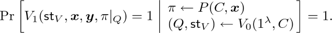
• Soundness. For any circuit family $\lbrace C_{\lambda } \rbrace _{\lambda \in {\mathbb {N}}}$ and any probabilistic Turing machine $P^*$ (called cheating prover), there exists a negligible function $\mathsf{negl}$ such that for every security parameter $\lambda \in {\mathbb {N}}$,

  

$\Diamond$

A PCP system is said to be linear if it satisfies an additional property that the proof is a linear function.

Definition 2

(Linear PCPs). Let (P, V) be any PCP system and $\lbrace D_{C} \rbrace _{C}$ be its proof domains. Then, (P, V) is said to be linear if for every arithmetic circuit $C$ and input $\varvec{x}$ of $C$,

2.4 No-signaling PCPs

No-signaling PCPs [39, 40] are PCP systems that guarantee soundness against a stronger class of cheating provers called no-signaling cheating provers. The main difference between no-signaling cheating provers and normal cheating provers in that, while a normal cheating prover is required to output a PCP proof $\pi ^*$ before seeing queries Q, a no-signaling cheating prover is allowed to output $\pi ^*$ after seeing Q. There is however a restriction on the distribution of $\pi ^*$; roughly speaking, it is required that for any (not too large) sets $Q, Q'$ such that $Q' \subset Q$, the distribution of $\pi ^*|_{Q'}$ when the queries are Q should be indistinguishable from the distribution of it when the queries are $Q'$. The formal definition is given below. (The following definition is the “computational” variant of the definition, which is given by Brakerski et al. [20]).

Definition 3

(No-signaling cheating prover). Let (P, V) be any PCP system, $\lbrace D_{C} \rbrace _{C}$ and $\lbrace \varSigma _{C} \rbrace _{C}$ be the proof domains and proof alphabets of (P, V), $\lbrace C_{\lambda } \rbrace _{\lambda \in {\mathbb {N}}}$ be any circuit family, and $P^*$ be any probabilistic Turing machine with the following syntax.

• Given the security parameter $\lambda \in {\mathbb {N}}$, the circuit $C_{\lambda }$, and a set of queries $Q \subset D_{C_{\lambda }}$ as input, $P^*$ outputs an input $\varvec{x}$ of $C_{\lambda }$, an output $\varvec{y}$ of $C_{\lambda }$, and a partial function $\pi ^*: Q \rightarrow \varSigma _{C_{\lambda }}$. (Note that $\pi ^*$ can be viewed as a PCP proof whose domain is restricted to Q).

Then, for any polynomial $\kappa _{\mathrm {max}}$, $P^*$ is said to be a $\kappa _{\mathrm {max}}$-wise (computational) no-signaling cheating prover if for any $\textsc {ppt}$ Turing machine ${\mathcal {D}}$, there exists a negligible function $\mathsf{negl}$ such that for every $\lambda \in {\mathbb {N}}$, every $Q, Q' \subset D_{C_{\lambda }}$ such that $Q' \subset Q$ and $|Q | \le \kappa _{\mathrm {max}}(\lambda )$, and every $z\in \lbrace 0,1 \rbrace ^{\mathsf{poly}(\lambda )}$,

$\Diamond$

Now, we define no-signaling PCPs as the PCP systems that satisfy soundness according to the following definition.

Definition 4

(Soundness against no-signaling cheating provers). Let (P, V) be any PCP system and $\kappa _{\mathrm {max}}$ be any polynomial. Then, (P, V) is said to be sound against $\kappa _{\mathrm {max}}$ -wise (computational) no-signaling cheating provers if for any circuit family $\lbrace C_{\lambda } \rbrace _{\lambda \in {\mathbb {N}}}$ and $\kappa _{\mathrm {max}}$-wise no-signaling cheating prover $P^*$, there exists a negligible function $\mathsf{negl}$ such that for every $\lambda \in {\mathbb {N}}$,

$\Diamond$

3 Technical Overview

In this section, we give an overview of our no-signaling linear PCP system. Recall that our focus is on PCP systems for the correctness of arithmetic computation, which are PCP systems that take as input a tuple $(C, \varvec{x}, \varvec{y})$ and prove that $C(\varvec{x}) = \varvec{y}$ holds. We focus on arithmetic circuits over prime-order fields. Given a circuit $C$, we use ${\mathbb {F}}$ to denote the underlying finite field, $N$ to denote the number of the wires,⁸ $n$ to denote the number of the input gates, and $m$ to denote the number of the output gates. We assume that the first $n$ wires are the wires that takes the values of the input gates and the last $m$ ones are those that takes the value of the output gates. In this overview we focus on circuits with output length 1 (i.e., $m=1$).

3.1 Preliminary: Linear PCP of Arora et al. [4]

The construction and analysis of our PCP system is based on the linear PCP system of Arora et al. [4] (ALMSS linear PCP in short), so let us start by recalling it. We describe only the construction of ALMSS linear PCP below; good explanations of the analysis of ALMSS linear PCP can be found in, e.g., the textbook by Arora and Barak [3, Chap. 11.5].

Main Tool: Walsh–Hadamard Code. The main tool of ALMSS linear PCP system is Walsh–Hadamard code. Recall that Walsh–Hadamard code maps a string $\varvec{v}\in {\mathbb {F}}^{\ell }$ to the linear function $\textsf {WH}_{\varvec{v}}: \varvec{x} \mapsto \langle \varvec{v}, \varvec{x} \rangle$. A useful property of Walsh–Hadamard code is that errors on codewords can be easily “self-corrected.” In particular, if a function f is $(1-\delta )$-close to a linear function ${\hat{f}}$ (i.e., if there exists a linear function ${\hat{f}}$ such that ), we can evaluate ${\hat{f}}$ on any point $\varvec{x}\in {\mathbb {F}}^{\ell }$ with error probability $2\delta$ though the following simple probabilistic procedure.

$\underline{\mathbf{Algorithm \, {\textsf {Self-Correct}}^{{\varvec{f}}} ({{\varvec{x}}})}}$:

Choose random $\varvec{r}\in {\mathbb {F}}^{\ell }$ and output $f(\varvec{x}+\varvec{r}) - f(\varvec{r})$.

Construction of ALMSS Linear PCP. On input $(C, \varvec{x})$, the prover P computes the PCP proof as follows. First, P computes and then obtains the following system of quadratic equations over ${\mathbb {F}}$, which is designed so that it is satisfiable if and only if $C(\varvec{x}) = y$. Intuitively, the system has variables that represent the wire values of $C$, and the equations in the system guarantee that (1) the correct input values $\varvec{x} = (x_1, \ldots , x_{n})$ are assigned on the input gates, (2) each gate is correctly computed, and (3) the claimed output value y is assigned on the output gate. Formally, the system of equations is defined as follows.

• The variables are $\varvec{z} = (z_1, \ldots , z_{N})$.

• For each $i\in \lbrace 1,\ldots ,n \rbrace$, the system has the equation $z_i = x_i$.

• For each $i,j,k\in [N]$, the system has $z_i + z_j - z_k = 0$ if $C$ has an addition gate with input wire i, j and output wire k, and has $z_i \cdot z_j - z_k = 0$ if $C$ has a multiplication gate with input wire i, j and output wire k.

• The system has the equation $z_{N} = y$.

Let us denote this system of quadratic equations by $\varPsi = \lbrace \varPsi _i(\varvec{z}) = c_i \rbrace _{i\in [M]}$, where $M$ is the number of the equations. Then, P obtains the satisfying assignment $\varvec{w} = (w_1, \ldots , w_{N})$ of $\varPsi$ through the wire values of $C$ on $\varvec{x}$, and outputs the two linear functions and as the PCP proof.⁹ (In short, the PCP proof is Walsh–Hadamard encodings of $\varvec{w}$ and $\varvec{w}\,\otimes \,\varvec{w}$).

Next, on input $(C, \varvec{x}, y)$, the verifier V verifies the PCP proof as follows. First, V obtains the system of equations $\varPsi = \lbrace \varPsi _i(\varvec{z}) = c_i \rbrace _{i\in [M]}$. Then, V applies the following three tests on the PCP proof $\lambda$ times in parallel.

• 1. (Linearity Test). Choose random points $\varvec{r}_1, \varvec{r}_2 \in {\mathbb {F}}^{N}$ and $\varvec{r}'_1, \varvec{r}'_2 \in {\mathbb {F}}^{N^2}$ and check $\pi _f(\varvec{r}_1) + \pi _f(\varvec{r}_2) \overset{?}{=}\pi _f(\varvec{r}_1 + \varvec{r}_2)$ and $\pi _g(\varvec{r}'_1) + \pi _g(\varvec{r}'_2) \overset{?}{=}\pi _g(\varvec{r}'_1 + \varvec{r}'_2)$.

• 2. (Tensor-Product Test). Choose two random points $\varvec{r}_1, \varvec{r}_2\in {\mathbb {F}}^{N}$, run $a_{\varvec{r}_1} \leftarrow \textsf {Self}\textsf {-}\textsf {Correct}^{\pi _f}(\varvec{r}_1)$, $a_{\varvec{r}_2} \leftarrow \textsf {Self}\textsf {-}\textsf {Correct}^{\pi _f}(\varvec{r}_2)$, $a_{\varvec{r}_1\otimes \varvec{r}_2} \leftarrow \textsf {Self}\textsf {-}\textsf {Correct}^{\pi _g}(\varvec{r}_1\otimes \varvec{r}_2)$, and check $a_{\varvec{r}_1} a_{\varvec{r}_2} \overset{?}{=}a_{\varvec{r}_1\otimes \varvec{r}_2}$.

• 3. (SAT Test). Choose a random point $\varvec{\sigma } = (\sigma _1, \ldots , \sigma _{M}) \in {\mathbb {F}}^{M}$, compute a quadratic function , run $a_{\varvec{\psi _{\varvec{\sigma }}}} \leftarrow \textsf {Self}\textsf {-}\textsf {Correct}^{\pi _f}(\varvec{\psi _{\varvec{\sigma }}})$, $a_{\varvec{\psi _{\varvec{\sigma }}'}} \leftarrow \textsf {Self}\textsf {-}\textsf {Correct}^{\pi _g}(\varvec{\psi _{\varvec{\sigma }}'})$ for the coefficient vectors $\varvec{\psi _{\varvec{\sigma }}}, \varvec{\psi _{\varvec{\sigma }}'}$ such that $\langle \varvec{\psi _{\varvec{\sigma }}}, \varvec{z} \rangle + \langle \varvec{\psi _{\varvec{\sigma }}'}, \varvec{z}\otimes \varvec{z} \rangle = \varPsi _{\varvec{\sigma }}(\varvec{z})$, and check $a_{\varvec{\psi _{\varvec{\sigma }}}} + a_{\varvec{\psi _{\varvec{\sigma }}'}} \overset{?}{=}c_{\varvec{\sigma }}$, where .

Comment: Roughly speaking, Linearity Test guarantees that $\pi _f, \pi _g$ are close to some linear functions ${\hat{f}}, {\hat{g}}$, Tensor-Product Test guarantees that ${\hat{f}}, {\hat{g}}$ are Welsh–Hadamard encodings of $\tilde{\varvec{w}}, \tilde{\varvec{w}}\otimes \tilde{\varvec{w}}$ for some $\tilde{\varvec{w}}\in {\mathbb {F}}^{N}$, and SAT Test guarantees that $\tilde{\varvec{w}}$ is the satisfying assignment of $\varPsi$, which implies that $\varPsi$ is satisfiable and thus the statement is true. (In Tensor-Product Test and SAT Test, $\textsf {Self}\textsf {-}\textsf {Correct}$ is used so that, if $\pi _f, \pi _g$ are indeed close to some linear functions ${\hat{f}}, {\hat{g}}$, the verifier can evaluate ${\hat{f}}, {\hat{g}}$ through $\pi _f, \pi _g$ with high probability). We refer the readers to [3, Chap. 11.5] for details of the analysis of ALMSS linear PCP.

V accepts the proof if it passes these three tests in all the $\lambda$ parallel trials. It can be verified by inspection that, as required in Definition 1, the verifier can be decomposed into $V_0$ and $V_1$, where $V_0$ samples queries to the tests and $V_1$ verifies the answers from the PCP proof. (Note that $V_0$ can sample all queries before knowing $\varvec{x}$ and y since the coefficient vectors $\varvec{\psi _{\varvec{\sigma }}}, \varvec{\psi _{\varvec{\sigma }}'}$ in SAT Test can be computed from $C$).

3.2 Construction of Our No-signaling Linear PCP

The construction of our PCP system, (P, V), is essentially identical with that of ALMSS linear PCP. There is a slight difference in the verifier algorithm (in our PCP system, $\textsf {Self}\textsf {-}\textsf {Correct}$ samples many candidates of the self-corrected values and takes the majority), but we ignore this difference in this overview. It can be verified by inspection that the running time of P is $\mathsf{poly}(|C |)$, the running time of $V_0$ is $\mathsf{poly}(\lambda + |C |)$, and the running time of $V_1$ is $\mathsf{poly}(\lambda + |\varvec{x} | + |\varvec{y} |)$.

3.3 Analysis of Our PCP

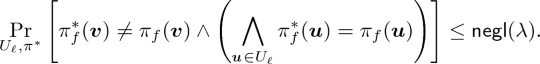
Our goal is to show that our PCP system (P, V) is sound against $\kappa _{\mathrm {max}}$-wise no-signaling cheating provers for sufficiently large polynomial $\kappa _{\mathrm {max}}$. That is, our goal is to show that for every circuit family $\lbrace C_{\lambda } \rbrace _{\lambda \in {\mathbb {N}}}$ and every $\kappa _{\mathrm {max}}$-wise no-signaling cheating prover $P^*$, we have

(1)

for every $\lambda \in {\mathbb {N}}$.

Toward this goal, for any sufficiently large $\kappa _{\mathrm {max}}$ and any $\kappa _{\mathrm {max}}$-wise no-signaling cheating prover $P^*$, we assume that we have

(2)

for infinitely many $\lambda \in {\mathbb {N}}$ (let $\varLambda$ be the set of those $\lambda$’s) and show that we have

(3)

for every sufficiently large $\lambda \in \varLambda$. Clearly, showing Eq. (3) while assuming Eq. (2) is sufficient for showing Eq. (1) (this is because it implies that for every polynomial $\mathsf{poly}$, either we have $V_1 (\textsf {st}_{V}, \varvec{x}, y, \pi ^*) = 1$ with probability at most $1/\mathsf{poly}(\lambda )$ or we have $C_{\lambda }(\varvec{x}) \ne y$ with probability at most $1/\mathsf{poly}(\lambda )$ for each sufficiently large $\lambda \in {\mathbb {N}}$).

To explain the overall structure of our analysis, we first show Eq. (3) while assuming the following (very strong) simplifying assumptions instead of Eq. (2).

Simplifying Assumption 1

$P^*$ convinces the verifier V with overwhelming probability. That is, we have

(4)

for infinitely many $\lambda \in {\mathbb {N}}$. (In what follows, we override the definition of $\Lambda$ and let it be the set of these $\lambda$’s). $\Diamond$

Simplifying Assumption 2

$P^*$ creates a proof that passes each of Linearity Test, Tensor-Product Test, and SAT Test on any points with overwhelming probability. That is, for every sufficiently large $\lambda \in \Lambda$, we have the following. (We assume without loss of generality that $P^*$ always outputs a PCP proof $\pi ^*= (\pi ^*_f, \pi ^*_g)$ that consists of two functions $\pi ^*_f$ and $\pi ^*_g$).

• (Linearity of $\pi ^*_f$ ). For every $\varvec{u}, \varvec{v} \in {\mathbb {F}}^{N}$,

  

  (5)

• (Linearity of $\pi ^*_g$ ). For every $\varvec{u}, \varvec{v} \in {\mathbb {F}}^{N^2}$,

  

  (6)

• (Tensor-Product Consistency of $\pi ^*_f, \pi ^*_g$ ). For every $\varvec{u}, \varvec{v} \in {\mathbb {F}}^{N}$,

  

  (7)

• (SAT Consistency of $\pi ^*_f, \pi ^*_g$ ). For every $\varvec{\sigma }\in {\mathbb {F}}^{M}$,

  

  (8)

  $\Diamond$

At the end of this subsection, we explain how we remove these simplifying assumptions in the actual analysis.

Under the above two simplifying assumptions, we obtain Eq. (3) as follows. Notice that if the statement is true and the PCP proof is correctly generated, then the first part of PCP proof, $\pi _f(\varvec{v}) = \langle \varvec{v}, \varvec{w} \rangle$, is the linear function whose coefficient vector is the satisfying assignment $\varvec{w}$ of the system of equations $\varPsi = \lbrace \varPsi _i(\varvec{z}) = c_i \rbrace _{i\in [M]}$, so we can recover the satisfying assignment on any variable $z_i$ by appropriately evaluating $\pi _f$. (Concretely, given $\pi _f$, we can obtain the satisfying assignment on $z_i$ by evaluating $\pi _f$ on $\varvec{e}_i = (0, \ldots , 0, 1, 0, \ldots , 0) \in {\mathbb {F}}^{N}$, where only the i-th element of $\varvec{e}_i$ is 1). Now, we first observe that we can obtain Eq. (3) by showing that the “cheating assignment” that we recover from the cheating prover $P^*$ is “correct” in the following two ways.

• 1. The assignment on $z_{N}$ (which represents the value of the output gate) is equal to the claimed output value. That is, for every sufficiently large $\lambda \in \Lambda$,

  

  (9)

• 2. The assignment on $z_{N}$ is equal to the actual output value. That is, for every sufficiently large $\lambda \in \Lambda$,

  

  (10)

Indeed, given Eqs. (9) and (10), we can easily obtain Eq. (3) as follows: first, we obtain

by applying the union bound on Eqs. (9) and (10); then, we obtain Eq. (3) by using the no-signaling property of $P^*$ to argue that the probability of $C_{\lambda }(\varvec{x}) = y$ holding decreases only negligibly when the queries to $P^*$ are changed from $\lbrace \varvec{e}_{N} \rbrace$ to $\lbrace \varvec{e}_{N} \rbrace \cup Q$ and from $\lbrace \varvec{e}_{N} \rbrace \cup Q$ to Q.¹⁰ (Notice that the distinguisher in the no-signaling game can check $C_{\lambda }(\varvec{x}) \overset{?}{=}y$ efficiently). Therefore, to conclude the analysis (under the simplifying assumptions), it remains to prove Eqs. (9) and (10).

Step 1. Showing Consistency with the Claimed Computation. First, we explain how we obtain Eq. (9) under the simplifying assumptions on $P^*$.

To obtain Eq. (9), we prove a stronger claim on the cheating assignment. Recall that from the construction of $\varPsi = \lbrace \varPsi _i(\varvec{z}) = c_i \rbrace _{i\in [M]}$, each equation of $\varPsi$ is defined with at most three variables, and in particular each equation $\varPsi _i(\varvec{z}) = c_i$ can be written as $\sum _{j\in \lbrace \alpha ,\beta ,\gamma \rbrace } d_{j}z_{j} + \sum _{j,k\in \lbrace \alpha ,\beta ,\gamma \rbrace } d_{j,k}z_{j}z_{k} = c_i$ for some $\alpha ,\beta ,\gamma \in [N]$ ($\alpha< \beta < \gamma$), $d_{j}\in \lbrace -1,0,1 \rbrace$ ($j\in \lbrace \alpha , \beta , \gamma \rbrace$), and $d_{j,k}\in \lbrace -1,0,1 \rbrace$ ($j,k\in \lbrace \alpha , \beta , \gamma \rbrace$). Then, we consider the following claim.

$1'$.:

(Consistency with Claimed Computation) For any equation $\varPsi _i(\varvec{z}) = c_i$ of $\varPsi$, which can be written as

$$\begin{aligned} \sum _{j\in \lbrace \alpha ,\beta ,\gamma \rbrace } d_{j}z_{j} + \sum _{j,k\in \lbrace \alpha ,\beta ,\gamma \rbrace } d_{j,k}z_{j}z_{k} = c_i, \end{aligned}$$

the cheating assignment on $z_{\alpha }, z_{\beta }, z_{\gamma }$ is a satisfying assignment of this equation. That is, for every sufficiently large $\lambda \in \Lambda$ and every $i\in [M]$, we have

(11)

where ${\textsf {Consist}}_i(C_{\lambda }, \varvec{x}, y, \pi ^*)$ is the event that we have

$$\begin{aligned} \sum _{j\in \lbrace \alpha ,\beta ,\gamma \rbrace } d_{j}\pi ^*_f(\varvec{e}_j) + \sum _{j,k\in \lbrace \alpha ,\beta ,\gamma \rbrace } d_{j,k}\pi ^*_f(\varvec{e}_j)\pi ^*_f(\varvec{e}_k) = c_i. \end{aligned}$$

Clearly, this claim implies Eq. (9) since $\varPsi$ has the equation $z_{N} = y$.

Hence, we focus on showing the stronger claim that Eq. (11) holds. Fix any sufficiently large $\lambda \in \Lambda$ and any $i\in [M]$. First, since the cheating PCP proof passes SAT Test on any points (Eq. (8) of Simplifying Assumption 2), we have

(12)

where $\varvec{e}_{i} = (0, \ldots , 0, 1, 0, \ldots , 0)\in {\mathbb {F}}^{M}$. Second, since we have $\varvec{\psi }_{\varvec{e}_{i}} = \sum _{j\in \lbrace \alpha ,\beta ,\gamma \rbrace } d_{j}\varvec{e}_j$, $\varvec{\psi }'_{\varvec{e}_{i}} = \sum _{j,k\in \lbrace \alpha ,\beta ,\gamma \rbrace } d_{j,k}\varvec{e}_j\otimes \varvec{e}_k$, and $c_{\varvec{e}_{i}} = c_i$ from the definitions, Eq. (12) implies Eq. (11) if we have the following three items with overwhelming probability.¹¹

• $\pi ^*_f(\sum _{j\in \lbrace \alpha ,\beta ,\gamma \rbrace } d_{j}\varvec{e}_j) = \sum _{j\in \lbrace \alpha ,\beta ,\gamma \rbrace } d_{j}\pi ^*_f(\varvec{e}_j)$.

• $\pi ^*_g(\sum _{j,k\in \lbrace \alpha ,\beta ,\gamma \rbrace } d_{j,k}\varvec{e}_j\otimes \varvec{e}_k) = \sum _{j,k\in \lbrace \alpha ,\beta ,\gamma \rbrace } d_{j ,k}\pi ^*_g(\varvec{e}_j\otimes \varvec{e}_k)$.

• $\pi ^*_g(\varvec{e}_j\otimes \varvec{e}_k) = \pi ^*_f(\varvec{e}_j)\pi ^*_f(\varvec{e}_k)$ for every $j,k\in \lbrace \alpha ,\beta ,\gamma \rbrace$.

Now, we obtain Eq. (11) since these three items indeed hold with overwhelming probability due to Simplifying Assumption 2. (We use generalized versions of Eqs. (5) and (6) for the first two, and use Eq. (7) for the third one).

Step 2. Showing Consistency with the Actual Computation. Next, we explain how we obtain Eq. (10) under the simplifying assumptions on $P^*$.

Without loss of generality, we assume that arithmetic circuits are “layered,” i.e., the gates in a circuit can be partitioned into layers such that (1) the first layer consists of the input gates and the last layer consists of the output gate, and (2) the gates in the i-th layer have children in the $(i-1)$-th layer.

The overall strategy is to prove Eq. (10) by induction on the layers. For any circuit $C_{\lambda }$, let us use the following notations.

• $\ell _{\mathrm {max}}$ is the number of the layers, and $N_i$ is the number of the wires in layer i (i.e., the number of the wires from the gates in layer i). We assume that the numbering of the wires are consistent with the numbering of the layers, i.e., the first $N_1$ wires are those that are in the first layer, the next $N_2$ wires are those that are in the second layer, etc.

• $D_1, \ldots , D_{\ell _{\mathrm {max}}}$ are subset of ${\mathbb {F}}^{N}$ such that for every $\ell \in [\ell _{\mathrm {max}}]$,

  

  where . Notice that when the first part of the correct PCP proof, $\pi _f(\varvec{v}) = \langle \varvec{v}, \varvec{w} \rangle$, is evaluated on $v_{\ell }\in D_{\ell }$, it returns a linear combination of the correct wire values of layer $\ell$.

Now, to prove Eq. (10), we show that the following three claims holds for every sufficiently large $\lambda \in \Lambda$.

• 1. The cheating PCP proof is equal to the correct PCP proof on random $\lambda$ points in $D_1$. That is,

  

  (13)

  where the probability is taken over $\varvec{u}_{1, i} \leftarrow D_{1}$ ($i\in [\lambda ]$), , and $(\varvec{x}, y, \pi ^*) \leftarrow P^*(1^{\lambda }, C_{\lambda }, U_1)$, and $\pi _f$ is the correct PCP proof that is generated by .

• 2. For every $\ell \in [\ell _{\mathrm {max}}]$, if the cheating PCP proof is equal to the correct PCP proof on random $\lambda$ points in $D_{\ell }$, they are also equal on any point in $D_{\ell }$. That is, for any $\varvec{v}\in D_{\ell }$,

  

  (14)

  where the probability is taken over $\varvec{u}_{\ell , i} \leftarrow D_{\ell }$ ($i\in [\lambda ]$), , and $(\varvec{x}, y, \pi ^*) \leftarrow P^*(1^{\lambda }, C_{\lambda }, \lbrace \varvec{v} \rbrace \cup U_{\ell })$.

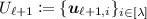
• 3. For every $\ell \in [\ell _{\mathrm {max}}-1]$, if the cheating PCP proof is equal to the correct PCP proof on random $\lambda$ points in $D_{\ell }$, they are also equal on random $\lambda$ points in $D_{\ell +1}$. That is,

  

  (15)

  where the probability is taken over $\varvec{u}_{\ell , i} \leftarrow D_{\ell }$ ($i\in [\lambda ]$), $\varvec{u}_{\ell +1, i} \leftarrow D_{\ell +1}$ ($i\in [\lambda ]$), , , and $(\varvec{x}, y, \pi ^*) \leftarrow P^*(1^{\lambda }, C_{\lambda }, U_{\ell }\cup U_{\ell +1})$.

Observe that we can indeed obtain Eq. (10) from the above three claims since Eq. (14) implies that we can obtain Eq. (10) by just showing

(this is because we have $\pi _f(\varvec{e}_{N}) = w_{N} = C_{\lambda }(\varvec{x})$ from the construction of our PCP), and we can obtain this inequation by repeatedly using Eq. (15) on top of Eq. (13).¹² Thus, what remain to prove are Eqs. (13), (14), (15).

• 1. To obtain Eq. (13), we first use the linearity of the cheating PCP proof (Eq. (5) of Simplifying Assumption 2) to argue that, since any $v\in D_1$ can be written as a linear combination of $\varvec{e}_1, \ldots , \varvec{e}_{n}\in {\mathbb {F}}^{N}$ (recall that we have $N_1 = n$), we can obtain Eq. (13) by just showing that for every $i\in [n]$ we have $\pi ^*_f(\varvec{e}_i) = \pi _f(\varvec{e}_i)$ with overwhelming probability. Then, we observe that, since we have $\pi _f(\varvec{e}_i) = w_i = x_i$ for every $i\in [n]$ from the construction of our PCP, it suffices to show that for every $i\in [n]$ we have $\pi ^*_f(\varvec{e}_i) = x_i$ with overwhelming probability, which we already showed as the consistency with the claimed computation (Eq. (11) in Step 1).

• 2. To obtain Eq. (14), we consider a mental experiment where $U_{\ell } = \lbrace \varvec{u}_{\ell , i} \rbrace _{i\in [\lambda ]}$ is sampled as follows: for each $i\in [\lambda ]$, choose random $\varvec{r}_i\in D_{\ell }$ and $b_i\in \lbrace 0,1 \rbrace$ and then define $\varvec{u}_{\ell , i}$ by if $b_i = 0$ and by if $b_i = 1$. Since each $\varvec{u}_{\ell , i}$ is still uniformly distributed, it suffices to show Eq. (14) w.r.t. this mental experiment; in addition, due to the no-signaling property of $P^*$, we can further change the experiment so that $\pi ^*$ is obtained by $(\varvec{x}, y, \pi ^*) \leftarrow P^*(1^{\lambda }, C_{\lambda }, \lbrace v \rbrace \cup \lbrace \varvec{r}_i, \varvec{v}+\varvec{r}_{\ell , i} \rbrace _{i\in [\lambda ]})$. Now, we obtain Eq. (14) by observing the following.

  • (a) Equation (14) is implied by

    

    (16)

    (We assume that $\wedge _{\varvec{u}\in U_{\ell }} \pi ^*_f(\varvec{u}) = \pi _f(\varvec{u})$ holds with high probability, which is indeed the case in our situation).

  • (b) We can obtain Eq. (16) by combining the following two observations. First, we have $\pi ^*_f(\varvec{v}) \ne \pi _f(\varvec{v})$ only when we have $\pi ^*_f(\varvec{v}+\varvec{r}_i) \ne \pi _f(\varvec{v}+\varvec{r}_i)$ or $\pi ^*_f(\varvec{r}_i) \ne \pi _f(\varvec{r}_i)$ for every $i\in [\lambda ]$ (this is because we have $\pi ^*_f(\varvec{v}) = \pi ^*_f(\varvec{v}+\varvec{r}_i)-\pi ^*_f(\varvec{r}_i)$ for every $i\in [\lambda ]$ from the linearity of the cheating PCP proof¹³ (Eq. (5) of Simplifying Assumption 2)). Second, when we have $\pi ^*_f(\varvec{v}+\varvec{r}_i) \ne \pi _f(\varvec{v}+\varvec{r}_i)$ or $\pi ^*_f(\varvec{r}_i) \ne \pi _f(\varvec{r}_i)$ for every $i\in [\lambda ]$, we have $\wedge _{\varvec{u}\in U_{\ell }} \pi ^*_f(\varvec{u}) = \pi _f(\varvec{u})$ with probability at most $2^{-\lambda }$ since each $\varvec{u}_{\ell , i}$ is defined by taking either $\varvec{r}_i$ or $\varvec{v}+\varvec{r}_i$ randomly.

• 3. To obtain Eq. (15), we first use the linearity of the cheating PCP proof (Eq. (5) of Simplifying Assumption 2) and the union bound to argue, just like when we show Eq. (13), that we can obtain Eq. (15) by just showing that for every $k\in \lbrace N_{\le \ell }+1, \ldots , N_{\le \ell }+N_{\ell +1} \rbrace$ we have $\pi ^*_f(\varvec{e}_k) = \pi _f(\varvec{e}_k)$ with overwhelming probability (where the probability is conditioned on ${{{\mathrm{\bigwedge }}}}_{\varvec{u}\in U_{\ell }} \pi ^*_f(\varvec{u}) = \pi _f(\varvec{u})$). Let us focus, for simplicity, on the case that k is the output wire of a multiplication gate in the $(\ell +1)$-th layer, where the input wires are i and j in the $\ell$-th layer. Then, we observe that we have $\pi ^*_f(\varvec{e}_k) = \pi _f(\varvec{e}_k)$ if we have

  $$\begin{aligned} \pi ^*_f(\varvec{e}_k) = \pi ^*_f(\varvec{e}_i)\pi ^*_f(\varvec{e}_j)&\text {and}&\pi ^*_f(\varvec{e}_i) = \pi _f(\varvec{e}_i) \wedge \pi ^*_f(\varvec{e}_j) = \pi _f(\varvec{e}_j) \end{aligned}$$

  (this is because these two items imply that $\pi ^*_f(\varvec{e}_k) = \pi ^*_f(\varvec{e}_i)\pi ^*_f(\varvec{e}_j) = \pi _f(\varvec{e}_i)\pi _f(\varvec{e}_j) = \pi _f(\varvec{e}_k)$, where the last equality holds since $\pi _f(\varvec{e}_i), \pi _f(\varvec{e}_j), \pi _f(\varvec{e}_k)$ are the satisfying assignment on $z_i, z_j, z_k$ of $\varPsi$, which has the equation $z_iz_j-z_k=0$). Finally, we observe that the first item holds with overwhelming probability since the cheating proof is consistent with the claimed computation (Eq. (11) in Step 1) and that the second item holds with overwhelming probability due to Eq. (14) and the union bound (both probabilities are conditioned on ${{{\mathrm{\bigwedge }}}}_{\varvec{u}\in U_{\ell }} \pi ^*_f(\varvec{u}) = \pi _f(\varvec{u})$).

How to Remove the Simplifying Assumptions. In the actual analysis, we remove Simplifying Assumption 1 in the same way as previous works (such as [20, 40]), namely by considering a “relaxed verifier” that accepts a PCP proof even when the proof fails to pass a small number of the tests. (Concretely, we consider a verifier that accepts a proof as long as the proof passes the three tests in at least $\lambda -\mu$ trials, where $\mu = \varTheta (\log ^2\lambda )$). We use the same argument as the previous works to show that if a cheating prover fools the original verifier with non-negligible probability, there exists another cheating prover that fools the relaxed verifier with overwhelming probability.

As for Simplifying Assumption 2, we remove it by considering the self-corrected version of the cheating proof, i.e., the proof that is obtained by applying $\textsf {Self}\textsf {-}\textsf {Correct}$ on the cheating proof $\pi ^*$. Our key observation is that an existing analysis of Linearity Test can be naturally extended so that it works even in the no-signaling PCP setting as long as we change the goal to showing that the self-corrected cheating proof passes Linearity Test on any points. (In the standard PCP setting, the goal of Linearity Test is to guarantee that the cheating proof is close to a linear function). Once we show that the self-corrected cheating proof passes Linearity Test on any points, it is relatively easy to show that it also passes Tensor-Product Test and SAT Test on any points.

3.4 Comparison with Previous Analysis

The high level structure of our analysis (under the abovementioned simplifying assumptions) is the same as the analysis of previous non-linear no-signaling PCPs, namely those of Kalai et al. [40] and the subsequent works. Specifically, like these works, we show $C_{\lambda }(\varvec{x}) = y$ by showing that we have $\pi ^*(\varvec{e}_{N}) = y$ and $\pi ^*(\varvec{e}_{N}) = C_{\lambda }(\varvec{x})$ simultaneously, and show $\pi ^*(\varvec{e}_{N}) = C_{\lambda }(\varvec{x})$ by induction on layers of $C_{\lambda }$. (In the latter part, we in particular follow the presentation by Paneth and Rothblum [47]).

A notable difference between our analysis and the previous one (other than the differences due to the use of linear PCPs rather than polynomially long PCP) is that our analysis does not require that the statement is represented as an “augmented layered circuit,” and only requires that it is represented as a layered circuit. More concretely, while the previous analysis requires that each layer of the circuit is augmented with an additional circuit that computes a low-degree extension of the wire values of the layer and then applies low-degree tests on the low-degree extension, our analysis does not require such augmentation and only requires that the circuit is layered. At a high level, we do not require this augmentation since in the induction for showing $\pi ^*(\varvec{e}_{N}) = C_{\lambda }(\varvec{x})$ (Step 2 in the previous subsection), we show that the cheating PCP proof is equal to the correct proof rather than just showing that the wire values that are recovered from the cheating PCP proof are equal to the correct ones. (That is, we do not require the augmentation of the circuit since we consider a stronger claim in the induction, which allows us to use a stronger assumption in the inductive step).

4 Construction of Our No-signaling Linear PCP for ${\mathcal {P}}$

In this section, we describe our no-signaling linear PCP system (P, V) for the correctness of arithmetic-circuit computation. Let $C: {\mathbb {F}}^{n} \rightarrow {\mathbb {F}}^{m}$ be an arithmetic circuit over a finite field ${\mathbb {F}}$ of prime order, and $\varvec{x} = (x_1, \ldots , x_{n}) \in {\mathbb {F}}^{n}$ be an input to $C$. Recall that we use $N$ to denote the number of wires in $C$ and assume that the first $n$ wires are the those that takes the values of the input gates and the last $m$ ones are those that takes the value of the output gates.

4.1 PCP Prover P

Given $(C, \varvec{x})$ as input, the PCP prover P first computes and then obtains the following system of quadratic equations over ${\mathbb {F}}$, which is designed so that it is satisfiable if and only if $C(\varvec{x}) = \varvec{y}$. Intuitively, the system has variables that represent the wire values of $C$, and the equations in the system guarantee that (1) the correct input values $\varvec{x} = (x_1, \ldots , x_{n})$ are assigned on the input gates, (2) each gate is correctly computed, and (3) the claimed output values $\varvec{y} = (y_1, \ldots , y_{m})$ are assigned on the output gates. Formally, the system of equations is defined as follows.

• The variables are $\varvec{z} = (z_1, \ldots , z_{N})$.

• For each $i\in \lbrace 1,\ldots ,n \rbrace$, the system has the equation $z_i = x_i$.

• For each $i,j,k\in [N]$, the system has $z_i + z_j - z_k = 0$ if the circuit $C$ has an addition gate with input wire i, j and output wire k, and has $z_iz_j - z_k = 0$ if $C$ has a multiplication gate with input wire i, j and output wire k.

• For each $i\in \lbrace 1, \ldots , m \rbrace$, the system has the equation $z_{N-m+i} = y_i$.

Let $M$ denote the number of the equations in the system $\varPsi$. Let the system be denoted by

$$\begin{aligned} \varPsi = \left\{ \begin{array}{l} \varPsi _1(\varvec{z}) = c_1\\ \vdots \\ \varPsi _{M}(\varvec{z}) = c_{M} \end{array} \right. , \end{aligned}$$

where each $c_i$ is an element in ${\mathbb {F}}$. For each $i\in [M]$, let $\varvec{\psi }_i\in {\mathbb {F}}^{N}$ and $\varvec{\psi '}_i\in {\mathbb {F}}^{N^2}$ be the coefficient vectors such that

$$\begin{aligned} \varPsi _i(\varvec{z}) = \langle \varvec{\psi }_i, \varvec{z} \rangle + \langle \varvec{\psi '}_i, \varvec{z}\otimes \varvec{z} \rangle . \end{aligned}$$

(17)

Let $\varvec{w} = (w_1, \ldots , w_{N})$ be the satisfying assignment of $\varPsi$. Let $f: {\mathbb {F}}^{N}\rightarrow {\mathbb {F}}$ and $g: {\mathbb {F}}^{N^2}\rightarrow {\mathbb {F}}$ be the linear functions that are defined by and . Then, the PCP prover P outputs the following linear function $\pi : {\mathbb {F}}^{N+N^2} \rightarrow {\mathbb {F}}$ as the PCP proof.

Remark 3

For simplicity, in what follows we usually think that P outputs two linear functions and as the PCP proof. This is without loss of generality since the verifier can evaluate f and g given access to $\pi$. $\Diamond$

4.2 PCP Verifier V

Given $(C, \varvec{x}, \varvec{y})$ as input, the PCP verifier V first computes the system $\varPsi$ in the same way as the PCP prover P. Next, given oracle access to the PCP proof $\pi _f$ and $\pi _g$, the PCP verifier does the following tests $\lambda$ times in parallel, and accepts the proof if all the tests in all the $\lambda$ trials are accepted.

• Linearity Test. Choose random points $\varvec{r}_1, \varvec{r}_2 \in {\mathbb {F}}^{N}$ and $\varvec{r}'_1, \varvec{r}'_2 \in {\mathbb {F}}^{N^2}$, and check the following.

  $$\begin{aligned} \pi _f(\varvec{r}_1) + \pi _f(\varvec{r}_2) \overset{?}{=}\pi _f(\varvec{r}_1 + \varvec{r}_2)&\text {and}&\pi _g(\varvec{r}'_1) + \pi _g(\varvec{r}'_2) \overset{?}{=}\pi _g(\varvec{r}'_1 + \varvec{r}'_2) . \end{aligned}$$

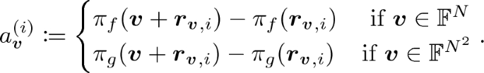
• Tensor-Product Test. Let $\textsf {Self}\textsf {-}\textsf {Correct}^{\pi }$ be the following algorithm.

  • $\underline{{\mathbf{Algorithm }\, {\textsf {Self-Correct}}^{\pi } ({{\varvec{v}}}\in {\mathbb {F}}^{N} \cup {\mathbb {F}}^{N^2}).}}$

    • 1. Choose $\lambda$ random points $\varvec{r}_{\varvec{v},1}, \ldots , \varvec{r}_{\varvec{v},\lambda }$ from ${\mathbb {F}}^{N}$ if $\varvec{v}\in {\mathbb {F}}^{N}$ and choose them from ${\mathbb {F}}^{N^2}$ if $\varvec{v}\in {\mathbb {F}}^{N^2}$.

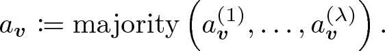
    • 2. For each $i\in [\lambda ]$, let

      

    • 3. Let

      

    • 4. Output $a_{\varvec{v}}$.

  Then, in Tensor-Product Test, choose two random points $\varvec{r}_1, \varvec{r}_2\in {\mathbb {F}}^{N}$, run

  $$\begin{aligned}&a_{\varvec{r}_1} \leftarrow \textsf {Self}\textsf {-}\textsf {Correct}^{\pi }(\varvec{r}_1),\\&a_{\varvec{r}_2} \leftarrow \textsf {Self}\textsf {-}\textsf {Correct}^{\pi }(\varvec{r}_2),\\&a_{\varvec{r}_1\otimes \varvec{r}_2} \leftarrow \textsf {Self}\textsf {-}\textsf {Correct}^{\pi }(\varvec{r}_1\otimes \varvec{r}_2), \end{aligned}$$

  and check the following.

  $$\begin{aligned} a_{\varvec{r}_1} a_{\varvec{r}_2} \overset{?}{=}a_{\varvec{r}_1\otimes \varvec{r}_2}. \end{aligned}$$

• SAT Test. Choose a random point $\varvec{\sigma } = (\sigma _1, \ldots , \sigma _{M}) \in {\mathbb {F}}^{M}$ and define a quadratic function $\varPsi _{\varvec{\sigma }}: {\mathbb {F}}^{N}\rightarrow {\mathbb {F}}$ as

  

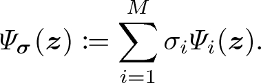
  Let $\varvec{\psi _{\varvec{\sigma }}}\in {\mathbb {F}}^{N}$ and $\varvec{\psi _{\varvec{\sigma }}'}\in {\mathbb {F}}^{N^2}$ be the coefficient vectors such that

  $$\begin{aligned} \varPsi _{\varvec{\sigma }}(\varvec{z}) = \langle \varvec{\psi _{\varvec{\sigma }}}, \varvec{z} \rangle + \langle \varvec{\psi _{\varvec{\sigma }}'}, \varvec{z}\otimes \varvec{z} \rangle . \end{aligned}$$

  (18)

  Let . Then, in SAT Test, run

  $$\begin{aligned}&a_{\varvec{\psi _{\varvec{\sigma }}}} \leftarrow \textsf {Self}\textsf {-}\textsf {Correct}^{\pi }(\varvec{\psi _{\varvec{\sigma }}}),\\&a_{\varvec{\psi _{\varvec{\sigma }}'}} \leftarrow \textsf {Self}\textsf {-}\textsf {Correct}^{\pi }(\varvec{\psi _{\varvec{\sigma }}'}) \end{aligned}$$

  and check the following.

  $$\begin{aligned} a_{\varvec{\psi _{\varvec{\sigma }}}} + a_{\varvec{\psi _{\varvec{\sigma }}'}} \overset{?}{=}c_{\varvec{\sigma }}. \end{aligned}$$

We remark that, formally, $V = (V_0, V_1)$ is a pair of two algorithms as required by Definition 1, where $V_0(1^{\lambda }, C)$ outputs a set of queries Q for the above tests along with its internal state $\textsf {st}_{V}$, and $V_1(\textsf {st}_{V}, \varvec{x}, \varvec{y}, \pi |_{Q})$ performs the above tests given the answers $\pi |_{Q}$ from the PCP proof. The internal state $\textsf {st}_{V}$ that $V_0$ outputs is $(\varvec{\sigma }_{\mathrm {in}}, \varvec{\sigma }_{\mathrm {out}})$, where

where it is assumed that the first $n$ equations in $\varPsi$ (i.e., the equations $\lbrace \varPsi _i(\varvec{z}) = c_i \rbrace _{i\in [n]}$) are those that are associated with the input gates (i.e., $\lbrace z_i = x_i \rbrace _{i\in [n]}$) and the last $m$ equations in $\varPsi$ (i.e. the equations $\lbrace \varPsi _{M-m+i}(\varvec{z}) = c_{M-m+i} \rbrace _{i\in [m]}$) are those that are associated with the output gates (i.e., $\lbrace z_{M-m+i} = y_i \rbrace _{i\in [n]}$). Note that $V_0(1^{\lambda }, C)$ can indeed choose all the queries in parallel (without knowing the input $\varvec{x}$ and the output $\varvec{y}$) since each of the queries is chosen independently of the results of other queries and in addition the coefficient vectors of the equations of $\varPsi$ (i.e., $\lbrace \varvec{\psi }_{i}, \varvec{\psi '}_{i} \rbrace _{i\in M}$) can be computed from the circuit $C$ in SAT Test. Also, note that $V_1(\textsf {st}_{V}, \varvec{x}, \varvec{y}, \pi |_{Q})$ can indeed perform the test (without knowing the circuit $C$) since $c_{\varvec{\sigma }} = \langle \varvec{\sigma }_{\mathrm {in}}, \varvec{x} \rangle + \langle \varvec{\sigma }_{\mathrm {out}}, \varvec{y} \rangle$ can be computed from $\textsf {st}_{V}$ in SAT Test.

Remark 4

(Query Complexity). By inspection, one can see that that the query complexity of V is $\kappa _{V}(\lambda ) {\mathop {=}\limits ^{\mathrm{def}}}\lambda (10\lambda +6)$. $\Diamond$

Remark 5

(Efficiency). By inspection, one can see that the running time of P is $\mathsf{poly}(|C |)$, the running time of $V_0$ is $\mathsf{poly}(\lambda + |C |)$, and the running time of $V_1$ is $\mathsf{poly}(\lambda + |\varvec{x} | + |\varvec{y} |)$. $\Diamond$

4.3 Security

In the full version of this paper [42], we prove the following theorem, which states the no-signaling soundness of our PCP system.

Theorem 1

(No-signaling Soundness of (P, V)). Let (P, V) be the PCP system in Sects. 4.1 and 4.2, $\lbrace C_{\lambda } \rbrace _{\lambda \in {\mathbb {N}}}$ be any circuit family, and $\kappa _{\mathrm {max}}$ be any polynomial such that $\kappa _{\mathrm {max}}(\lambda ) \ge 2\lambda \cdot \max (8\lambda +3, m_{\lambda }) + \kappa _{V}(\lambda )$, where $m_{\lambda }$ is the output length of $C_{\lambda }$ and $\kappa _{V}$ is the query complexity of (P, V). Then, for any $\kappa _{\mathrm {max}}$-wise (computational) no-signaling cheating prover $P^*$, there exists a negligible function $\mathsf{negl}$ such that for every $\lambda \in {\mathbb {N}}$,

5 Application: Delegating Computation in Preprocessing Model

In this section, we give an application of our no-signaling linear PCP system to a 2-message delegation scheme for ${\mathcal {P}}$ in the preprecessing model. As mentioned in Introduction, we obtain our delegation scheme by applying the transformation of Kalai et al. [39, 40] on our no-signaling linear PCP system.

We remark that our delegation scheme is actually non-interactive in the sense that, after the verifier’s message is computed and published in the (expensive) offline phase, anyone can prove a statement to the verifier in the online phase by sending a single message, and the same offline verifier message can be used for proving multiple statements in the online phase. Formally, this property is guaranteed due to the adaptive soundness of our delegation scheme, which guarantees that the soundness holds even when the statement to be proven is chosen after the verifier’s message.

5.1 Technical Overview

In this subsection, we give an overview of our delegation scheme. Those who are familiar with the transformation of Kalai et al. [39, 40] can skip this subsection.

Recall that in the setting of delegating computation, a computationally weak client asks a powerful server to perform a heavy computation, and the server returns the computation result to the client with a proof that the result is correct. Our focus is delegation schemes for arithmetic-circuit computation, so the statement to be proven by the server is of the form $(C, \varvec{x}, \varvec{y})$, which states that an arithmetic circuit $C$ outputs $\varvec{y}$ on input $\varvec{x}$. For simplicity, in this overview, we consider a static soundness setting where the statement is fixed before the verifier’s message is generated.

In our delegation scheme, we use the following two building blocks.

• Our no-signaling linear PCP system for deterministic arithmetic-circuit computation (Sect. 4).

• An additive homomorphic encryption scheme $\textsf {HE}$, which is an encryption scheme such that the message space is a finite group and that anyone can efficiently compute a ciphertext of $m_0+m_1$ from ciphertexts of any two messages $m_0, m_1$.

We assume that the message space of $\textsf {HE}$ is a finite field ${\mathbb {F}}$ of prime order, and consider delegation scheme for arithmetic circuits over this finite field ${\mathbb {F}}$.

The high-level structure of our delegation scheme is quite simple. When the statement is $(C, \varvec{x}, \varvec{y})$, our scheme roughly proceeds as follows.

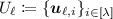
• 1. In the offline phase, the client firsts samples PCP queries Q of our PCP system, where $Q = \lbrace \varvec{q}_i \rbrace _{i\in [\kappa _{V}]}$ and $\varvec{q}_i = (q_{i,1}, \ldots , q_{i,N'})\in {\mathbb {F}}^{N'}$, where . Next, the client encrypts those queries by $\textsf {HE}$, where each query $\varvec{q}_i$ is encrypted under a fresh key. (That is, for each $i\in [\kappa _{V}]$, the client samples a key pair $(\textsf {pk}_i, \textsf {sk}_i)$ of $\textsf {HE}$ and encrypts each $q_{i,j}\in {\mathbb {F}}$ ($j\in [N']$) under the public-key $\textsf {pk}_i$). Finally, the verifier sends the resultant ciphertexts $\lbrace (\textsf {ct}_{i,1}, \ldots , \textsf {ct}_{i,N'}) \rbrace _{i\in [\kappa _{V}]}$ to the server.

• 2. Given the ciphertexts of the PCP queries $\lbrace (\textsf {ct}_{i,1}, \ldots , \textsf {ct}_{i,N'}) \rbrace _{i\in [\kappa _{V}]}$, the server obtain ciphertexts of the PCP answers by homomorphically evaluate the PCP oracle $\pi : {\mathbb {F}}^{N'} \rightarrow {\mathbb {F}}$ under the ciphertexts (since $\pi$ is a linear function, additive homomorphism of $\textsf {HE}$ suffices for evaluating $\pi$ ¹⁴), and then returns the resultant ciphertexts $\lbrace \tilde{\textsf {ct}}_i \rbrace _{i\in [\kappa _{V}]}$ to the client.

• 3. Given the ciphertexts of the PCP answers $\lbrace \tilde{\textsf {ct}}_i \rbrace _{i\in [\kappa _{V}]}$, the client obtains the PCP answers by decrypting $\lbrace \tilde{\textsf {ct}}_i \rbrace _{i\in [\kappa _{V}]}$ and then verifies the PCP answers by using the PCP decision algorithm.

The offline phase of our delegation scheme is expensive since the verifier query algorithm of our PCP system runs in time $\mathsf{poly}(\lambda +|C |)$, while the online phase is efficient since the verifier decision algorithm of our PCP system runs in time $\mathsf{poly}(\lambda +|\varvec{x} |+|\varvec{y} |)$. Very roughly speaking, the soundness of our scheme holds since, somewhat surprisingly, the semantic security of $\textsf {HE}$ directly guarantees that the server can answer to the PCP queries under the ciphertexts of $\textsf {HE}$ only in a no-signaling way. (Formally, in order to guarantee that the server is $\kappa _{\mathrm {max}}$-wise no-signaling for sufficiently large $\kappa _{\mathrm {max}}$, we need to change the above delegation scheme and add “dummy” queries to the PCP queries).

Using Multiplicative Homomorphic Encryption Rather Than Additive One. We can replace the additive homomorphic encryption scheme in the above scheme with a multiplicative one over prime-order bilinear group as follows: we replace the scheme so that, instead of encrypting the PCP queries $\lbrace (q_{i,1}, \ldots , q_{i,N}) \rbrace _{i\in [\kappa _{V}]}$ directly, the client encrypts $\lbrace g^{q_{i,1}}, \ldots , g^{q_{i,N}} \rbrace$, where g is a generator of the bilinear group, and the server homomorphically evaluates the PCP oracle in the exponent of g using the multiplicative homomorphic property of $\textsf {HE}$. Since the PCP verification algorithm only involves quadratic tests on the PCP answers, the client can verify the PCP answers even when the PCP answers are encoded in the exponent of g. (Unfortunately, the security analysis cannot be straightforwardly modified to work for this modified scheme).

5.2 Preliminaries

In this subsection, we first give the definition of delegation scheme and next give the definition of homomorphic encryption schemes.

Preprocessing Non-interactive Delegation Scheme. For concreteness, we focus our attention on 2-message delegation schemes with adaptive soundness, or in other words, non-interactive delegation schemes in the preprocessing model where the preprocess consists of a single message from the verifier. We remark that the following definition is essentially identical with the definition of preprocessing SNARGs (e.g., [16]) as well as the definition of adaptively sound 2-message delegation schemes of [7, 20]. The difference is that the following definition is tailored for deterministic arithmetic circuit computation.

A preprocessing non-interactive delegation scheme consists of three polynomial-time algorithms $(\textsf {Gen}, \textsf {Prove}, \textsf {Verify})$ with the following syntax.

• $\textsf {Gen}$ is a probabilistic algorithm such that on input the security parameter $1^{\lambda }$ and an arithmetic circuit C, it outputs a public-key $\textsf {pk}$ and a secret key $\textsf {sk}$.

• $\textsf {Prove}$ is a deterministic algorithm such that on input the public-key $\textsf {pk}$, the circuit $C$, and an input $\varvec{x}$ of $C$, it outputs a proof $\textsf {pr}$.

• $\textsf {Verify}$ is a deterministic algorithm such that on input the secret key $\textsf {sk}$, the input $\varvec{x}$, the output $\varvec{y}$, and the proof $\textsf {pr}$, it outputs a bit $b\in \lbrace 0,1 \rbrace$.

The execution of preprocessing non-interactive delegation schemes is separated into two phases, the offline phase and the online phase.

• Offline phase: First, the verifier obtains an arithmetic circuit $C$ that it wants to let the prover compute. Next, the verifier obtains $(\textsf {pk}, \textsf {sk})$ by running $\textsf {Gen}$ on $C$ and sends $\textsf {pk}$ to the prover. After executing $\textsf {Gen}$, the prover can erase the circuit $C$.

• Online phase: The prover, on input $\varvec{x}$ (which is obtained either from the verifier or from any other process), computes the output $\varvec{y} = C(\varvec{x})$ and the proof $\textsf {pr}= \textsf {Prove}(\textsf {pk}, C, \varvec{x})$ and then sends $(\varvec{x}, \varvec{y}, \textsf {pr})$ to the verifier. Given $(\varvec{x}, \varvec{y}, \textsf {pr})$, the verifier verifies the proof by running $\textsf {Verify}(\textsf {sk}, \varvec{x}, \varvec{y}, \textsf {pr})$. The online phase can be repeated multiple times on the same public key and secret key (see Remark 6 below).

Note that delegation scheme is meaningful only when the running time of $\textsf {Verify}$ is much smaller than the time that is needed for computing $C(\varvec{x})$.

The security requirements of preprocessing non-interactive delegation schemes are the following.

• Correctness. For every security parameter $\lambda \in {\mathbb {N}}$, arithmetic circuit $C$, input $\varvec{x}$ of $C$, and the output ,

  

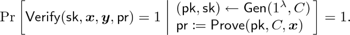
• Soundness. For every circuit family $\lbrace C_{\lambda } \rbrace _{\lambda \in {\mathbb {N}}}$ and $\textsc {ppt}$ adversary ${\mathcal {A}}$, there exists a negligible function $\mathsf{negl}$ such that for every $\lambda \in {\mathbb {N}}$,

  

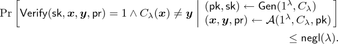
Remark 6

It is easy to see that if a delegation scheme is sound w.r.t. the above definition, it remains sound even when the same $(\textsf {pk}, \textsf {sk})$ is used for generating multiple proofs as long as the results of the verification are kept secret against the cheating provers (or, equivalently, as long as a new public-key–secret-key pair is generated when the verification of a proof is rejected).¹⁵ $\Diamond$

Homomorphic Encryption. A public-key encryption scheme consists of three polynomial-time algorithms $(\textsf {Gen}, \textsf {Enc}, \textsf {Dec})$ with the following syntax.

• $\textsf {Gen}$ is a probabilistic algorithm such that on input the security parameter $1^{\lambda }$, it outputs a public-key $\textsf {pk}$ and a secret key $\textsf {sk}$.

• $\textsf {Enc}$ is a probabilistic algorithm such that on input the public-key $\textsf {pk}$ and a message $m\in {\mathbb {F}}$, it outputs a ciphertext $\textsf {ct}$. (It is assumed that $\textsf {pk}$ contains the information of a finite field ${\mathbb {F}}$, which works as the message space).

• $\textsf {Dec}$ is a deterministic algorithm such that on input the secret-key $\textsf {sk}$ and the ciphertext $\textsf {ct}$, it outputs the plaintext m.

For any vector $\varvec{v}$, we denote by $\textsf {Enc}(\varvec{v})$ the element-wise encryption of $\varvec{v}$.

The following security notion of public-key encryption schemes is used in this paper (it is easy to see that the following security notion is implied by the standard CPA-security through a simple hybrid argument).

Definition 5

((multi-key multi-message) CPA-security). For every polynomial p and $\textsc {ppt}$ adversary ${\mathcal {A}}= ({\mathcal {A}}_0, {\mathcal {A}}_1, {\mathcal {A}}_2)$, there exists a negligible function $\mathsf{negl}$ such that for every security parameter $\lambda \in {\mathbb {N}}$ and every $z\in \lbrace 0,1 \rbrace ^{\mathsf{poly}(\lambda )}$,

$\Diamond$

A public-key encryption scheme $(\textsf {Gen}, \textsf {Enc}, \textsf {Dec})$ is additive homomorphic if it has an additional $\textsc {ppt}$ algorithm $\textsf {Eval}^{+}$ such that, on input $\textsf {ct}_1 \leftarrow \textsf {Enc}(m_1), \ldots , \textsf {ct}_{p(\lambda )} \leftarrow \textsf {Enc}(m_{p(\lambda )})$ for any $m_1, \ldots , m_{p(\lambda )}\in {\mathbb {F}}$ (where p is a polynomial), it outputs $\textsf {Enc}(\sum _{i=1}^{p(\lambda )} m_i)$. Formally, $\textsf {Eval}^+$ is required to satisfy the following property.

• Homomorphic Evaluation. For every polynomial p, every $\textsc {ppt}$ adversary ${\mathcal {A}}$, and every $\lambda \in {\mathbb {N}}$,

  

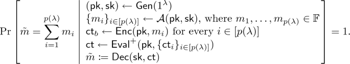
To simplify the exposition, for any two ciphertext $\textsf {ct}_0, \textsf {ct}_1$ under a public-key $\textsf {pk}$, we use $\textsf {ct}_0 + \textsf {ct}_1$ as a shorthand of $\textsf {Eval}^{+}(\textsf {pk}, \textsf {ct}_0, \textsf {ct}_1)$. Similarly, for any ciphertext $\textsf {ct}$ and a scalar $k\in {\mathbb {N}}$, we use $k\cdot \textsf {ct}$ as a shorthand of $\underbrace{\textsf {ct}+ \cdots + \textsf {ct}}_{k}$.

A public-key encryption scheme is multiplicative homomorphic if it has a $\textsc {ppt}$ algorithm $\textsf {Eval}^*$ that satisfies the above property w.r.t. multiplication over ${\mathbb {F}}$.

5.3 Our Result

Theorem 2

Assume the existence of an additive homomorphic encryption scheme over fields of prime order (i.e., over the additive group of the fields) or a multiplicative homomorphic encryption scheme over bilinear groups with prime order. Then, there exists a preprocessing non-interactive delegation scheme for polynomial-time arithmetic-circuit computation with the following efficiency.

• The running time of $\textsf {Gen}$ is $\mathsf{poly}(\lambda + |C |)$.

• The running time of $\textsf {Prove}$ is $\mathsf{poly}(\lambda + |C |)$.

• The running tine of $\textsf {Verify}$ is $\mathsf{poly}(\lambda + |\varvec{x} | + |\varvec{y} |)$.

Due to space limitations, we only give the description of our delegation scheme based on additive homomorphic encryption below, and refer the readers to the full version of this paper [42] for the proof of Theorem 2.

Let $(\textsf {HE.Gen}, \textsf {HE.Enc}, \textsf {HE.Dec})$ be the additive homomorphic encryption scheme and $(\textsf {PCP.P}, \textsf {PCP.V})$ be the PCP prover and verifiers of our PCP system (Sect. 4). Recall that our PCP system satisfies the following properties.

• It can handle arithmetic circuits over any prime-order fields. Furthermore, there exists a polynomial $\kappa _{\mathrm {max}}$ such that the soundness holds against any $\kappa _{\mathrm {max}}$-wise no-signaling adversaries.¹⁶

• For an arithmetic circuit $C$ over a finite filed ${\mathbb {F}}$, $\textsf {PCP.P}$ outputs a linear function $\pi : {\mathbb {F}}^{N+ N^2} \rightarrow {\mathbb {F}}$ as the PCP proof, where $N$ is the number of wires in $C$. (To simplify the notations, we let in what follows). Since $\pi$ is linear, there exists $d_1, \ldots , d_{N'}\in {\mathbb {F}}$ such that $\pi (\varvec{z}) = \sum _{i\in [N']}d_iz_i$.

• For an arithmetic circuit $C$ over a finite filed ${\mathbb {F}}$, $\textsf {PCP.V}_0$ outputs a set of queries $Q = \lbrace q_i \rbrace _{i\in [\kappa _{V}(\lambda )]}\subset {\mathbb {F}}^{N'}$ and a state $\textsf {st}_{V}\in {\mathbb {F}}^{n+m}$, where $\kappa _{V}$ is a polynomial (which is independent of $C$) and $n, m$ are the input and output length of $C$.

We assume that for every security parameter $\lambda$, the arithmetic circuit $C$ to be delegated is defined over a finite field ${\mathbb {F}}$ that is also the message space of $\textsf {HE}$.

Construction. The three algorithms $(\textsf {Gen}, \textsf {Prove}, \textsf {Verify})$ are defined as follows.

• Algorithm $\textsf {Gen}(1^{\lambda }, C)$

  • 1. Run $(Q, \textsf {st}_{V}) \leftarrow \textsf {PCP.V}_0(1^{\lambda }, C)$.

    Then, parse Q as $\lbrace \varvec{q}_i \rbrace _{i\in [\kappa _{V}(\lambda )]}$, where $\varvec{q}_i = (q_{i,1}, \ldots , q_{i,N'})\in {\mathbb {F}}^{N'}$.

  • 2. Define $\textsf {ct}_{1}, \ldots , \textsf {ct}_{\kappa _{\mathrm {max}}(\lambda )}$ as follows.

    • (a) Choose a random injective function $\tau : [\kappa _{V}(\lambda )] \rightarrow [\kappa _{\mathrm {max}}(\lambda )]$.

    • (b) Define $\textsf {ct}_i$ for each $i\in [\kappa _{\mathrm {max}}(\lambda )]$ by

      $$\begin{aligned} \textsf {ct}_{i} \leftarrow {\left\{ \begin{array}{ll} \textsf {HE.Enc}({\textsf {HE}}\textsf {.pk}_{i}, \varvec{q}_{\tau ^{-1}(i)}) &{} \text {(if }\exists i'\in [\kappa _{V}(\lambda )]\text { s.t. }\tau (i')=i)\\ \textsf {HE.Enc}({\textsf {HE}}\textsf {.pk}_{i}, \varvec{0}) &{} \text {(otherwise)} \end{array}\right. }, \end{aligned}$$

      where $({\textsf {HE}}\textsf {.pk}_i, {\textsf {HE}}\textsf {.sk}_i) \leftarrow \textsf {HE.Gen}(1^{\lambda })$ and .

  • 3. Output and .

• Algorithm $\textsf {Prove}(\textsf {pk}, C, \varvec{x})$

  • 1. Run $\pi \leftarrow \textsf {PCP.P}(C, \varvec{x})$.

    Let $d_1, \ldots , d_{N'}\in {\mathbb {F}}$ be such that $\pi (\varvec{z}) = \sum _{i\in [N']}d_iz_i$.

  • 2. Parse $\textsf {pk}$ as $(\textsf {ct}_1, \ldots , \textsf {ct}_{\kappa _{\mathrm {max}}(\lambda )})$, where $\textsf {ct}_i = (\textsf {ct}_{i,1}, \ldots , \textsf {ct}_{i, N'})$.

    Then, perform homomorphic operation to obtain

    

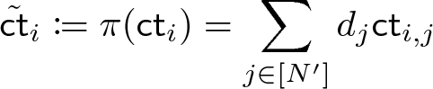
    for every $i\in [\kappa _{\mathrm {max}}(\lambda )]$.

  • 3. Output .

• Algorithm $\textsf {Verify}(\textsf {sk}, \varvec{x}, \varvec{y}, \textsf {pr})$

  • 1. Parse $\textsf {sk}$ as $(\textsf {st}_{V}, \tau , \lbrace {\textsf {HE}}\textsf {.sk}_i \rbrace _{i\in [\kappa _{\mathrm {max}}(\lambda )]})$, and $\textsf {pr}$ as $(\tilde{\textsf {ct}}_1, \ldots , \tilde{\textsf {ct}}_{\kappa _{\mathrm {max}}(\lambda )})$.

    Then, run for every $i\in [\kappa _{V}(\lambda )]$.

  • 2. Output .

Efficiency. By inspection, it can be verified that our delegation scheme indeed has the following efficiency.

• The running time of $\textsf {Gen}$ is $\mathsf{poly}(\lambda + |C |)$.

• The running time of $\textsf {Prove}$ is $\mathsf{poly}(\lambda + |C |)$.

• The running tine of $\textsf {Verify}$ is $\mathsf{poly}(\lambda + |\varvec{x} | + |\varvec{y} |)$.

References

Aiello, W., Bhatt, S., Ostrovsky, R., Rajagopalan, S.R.: Fast verification of any remote procedure call: short witness-indistinguishable one-round proofs for NP. In: Montanari, U., Rolim, J.D.P., Welzl, E. (eds.) ICALP 2000. LNCS, vol. 1853, pp. 463–474. Springer, Heidelberg (2000). https://doi.org/10.1007/3-540-45022-X_39
Ananth, P., Chen, Y.-C., Chung, K.-M., Lin, H., Lin, W.-K.: Delegating RAM computations with adaptive soundness and privacy. In: Hirt, M., Smith, A. (eds.) TCC 2016. LNCS, vol. 9986, pp. 3–30. Springer, Heidelberg (2016). https://doi.org/10.1007/978-3-662-53644-5_1
Arora, S., Barak, B.: Computational Complexity: A Modern Approach. Cambridge University Press, Cambridge (2009). http://theory.cs.princeton.edu/complexity/book.pdf
Arora, S., Lund, C., Motwani, R., Sudan, M., Szegedy, M.: Proof verification and the hardness of approximation problems. J. ACM 45(3), 501–555 (1998)
Arora, S., Safra, S.: Probabilistic checking of proofs: a new characterization of NP. J. ACM 45(1), 70–122 (1998)
Babai, L., Fortnow, L., Levin, L.A., Szegedy, M.: Checking computations in polylogarithmic time. In: 23rd ACM STOC, pp. 21–31. ACM Press, May 1991
Badrinarayanan, S., Kalai, Y.T., Khurana, D., Sahai, A., Wichs, D.: Succinct delegation for low-space non-deterministic computation. In: Diakonikolas, I., Kempe, D., Henzinger, M. (eds.) 50th ACM STOC, pp. 709–721. ACM Press, June 2018
Barak, B., Goldreich, O.: Universal arguments and their applications. SIAM J. Comput. 38(5), 1661–1694 (2009)
Ben-Sasson, E., Chiesa, A., Genkin, D., Tromer, E., Virza, M.: SNARKs for C: verifying program executions succinctly and in zero knowledge. In: Canetti, R., Garay, J.A. (eds.) CRYPTO 2013. LNCS, vol. 8043, pp. 90–108. Springer, Heidelberg (2013). https://doi.org/10.1007/978-3-642-40084-1_6
Ben-Sasson, E., Chiesa, A., Spooner, N.: Interactive oracle proofs. In: Hirt, M., Smith, A. (eds.) TCC 2016. LNCS, vol. 9986, pp. 31–60. Springer, Heidelberg (2016). https://doi.org/10.1007/978-3-662-53644-5_2
Ben-Sasson, E., Chiesa, A., Tromer, E., Virza, M.: Succinct non-interactive zero knowledge for a von Neumann architecture. In: Proceedings of the 23rd USENIX Security Symposium, San Diego, CA, USA, 20–22 August 2014, pp. 781–796 (2014)
Biehl, I., Meyer, B., Wetzel, S.: Ensuring the integrity of agent-based computations by short proofs. In: Rothermel, K., Hohl, F. (eds.) MA 1998. LNCS, vol. 1477, pp. 183–194. Springer, Heidelberg (1998). https://doi.org/10.1007/BFb0057658
Bitansky, N., et al.: The hunting of the SNARK. J. Cryptol. 30(4), 989–1066 (2017)
Bitansky, N., Canetti, R., Chiesa, A., Tromer, E.: Recursive composition and bootstrapping for SNARKS and proof-carrying data. In: Boneh, D., Roughgarden, T., Feigenbaum, J. (eds.) 45th ACM STOC, pp. 111–120. ACM Press, June 2013
Bitansky, N., Chiesa, A.: Succinct arguments from multi-prover interactive proofs and their efficiency benefits. In: Safavi-Naini, R., Canetti, R. (eds.) CRYPTO 2012. LNCS, vol. 7417, pp. 255–272. Springer, Heidelberg (2012). https://doi.org/10.1007/978-3-642-32009-5_16
Bitansky, N., Chiesa, A., Ishai, Y., Paneth, O., Ostrovsky, R.: Succinct non-interactive arguments via linear interactive proofs. In: Sahai, A. (ed.) TCC 2013. LNCS, vol. 7785, pp. 315–333. Springer, Heidelberg (2013). https://doi.org/10.1007/978-3-642-36594-2_18
Bitansky, N., Garg, S., Lin, H., Pass, R., Telang, S.: Succinct randomized encodings and their applications. In: Servedio, R.A., Rubinfeld, R. (eds.) 47th ACM STOC, pp. 439–448. ACM Press, June 2015
Boneh, D., Boyen, X., Shacham, H.: Short group signatures. In: Franklin, M. (ed.) CRYPTO 2004. LNCS, vol. 3152, pp. 41–55. Springer, Heidelberg (2004). https://doi.org/10.1007/978-3-540-28628-8_3
Boneh, D., Ishai, Y., Sahai, A., Wu, D.J.: Lattice-based SNARGs and their application to more efficient obfuscation. In: Coron, J.-S., Nielsen, J.B. (eds.) EUROCRYPT 2017. LNCS, vol. 10212, pp. 247–277. Springer, Cham (2017). https://doi.org/10.1007/978-3-319-56617-7_9
Brakerski, Z., Holmgren, J., Kalai, Y.T.: Non-interactive delegation and batch NP verification from standard computational assumptions. In: Hatami, H., McKenzie, P., King, V. (eds.) 49th ACM STOC, pp. 474–482. ACM Press, June 2017
Canetti, R., Chen, Y., Holmgren, J., Raykova, M.: Adaptive succinct garbled RAM or: how to delegate your database. In: Hirt, M., Smith, A. (eds.) TCC 2016. LNCS, vol. 9986, pp. 61–90. Springer, Heidelberg (2016). https://doi.org/10.1007/978-3-662-53644-5_3
Canetti, R., Holmgren, J.: Fully succinct garbled RAM. In: Sudan, M. (ed.) ITCS 2016, pp. 169–178. ACM, January 2016
Canetti, R., Holmgren, J., Jain, A., Vaikuntanathan, V.: Succinct garbling and indistinguishability obfuscation for RAM programs. In: Servedio, R.A., Rubinfeld, R. (eds.) 47th ACM STOC, pp. 429–437. ACM Press, June 2015
Chen, Y.C., Chow, S.S.M., Chung, K.M., Lai, R.W.F., Lin, W.K., Zhou, H.S.: Cryptography for parallel RAM from indistinguishability obfuscation. In: Sudan, M. (ed.) ITCS 2016, pp. 179–190. ACM, January 2016
Chiesa, A., Manohar, P., Shinkar, I.: Probabilistic checking against non-signaling strategies from linearity testing. Electronic Colloquium on Computational Complexity (ECCC), TR18-123 (2018). https://eccc.weizmann.ac.il/report/2018/123/
Chiesa, A., Manohar, P., Shinkar, I.: Testing linearity against non-signaling strategies. In: 33rd Computational Complexity Conference, CCC 2018, San Diego, California, USA, 22–24 June 2018, pp. 17:1–17:37 (2018)
Chung, K.-M., Kalai, Y., Vadhan, S.: Improved delegation of computation using fully homomorphic encryption. In: Rabin, T. (ed.) CRYPTO 2010. LNCS, vol. 6223, pp. 483–501. Springer, Heidelberg (2010). https://doi.org/10.1007/978-3-642-14623-7_26
Damgård, I., Faust, S., Hazay, C.: Secure two-party computation with low communication. In: Cramer, R. (ed.) TCC 2012. LNCS, vol. 7194, pp. 54–74. Springer, Heidelberg (2012). https://doi.org/10.1007/978-3-642-28914-9_4
Danezis, G., Fournet, C., Groth, J., Kohlweiss, M.: Square span programs with applications to succinct NIZK arguments. In: Sarkar, P., Iwata, T. (eds.) ASIACRYPT 2014. LNCS, vol. 8873, pp. 532–550. Springer, Heidelberg (2014). https://doi.org/10.1007/978-3-662-45611-8_28
Gennaro, R., Gentry, C., Parno, B.: Non-interactive verifiable computing: outsourcing computation to untrusted workers. In: Rabin, T. (ed.) CRYPTO 2010. LNCS, vol. 6223, pp. 465–482. Springer, Heidelberg (2010). https://doi.org/10.1007/978-3-642-14623-7_25
Gennaro, R., Gentry, C., Parno, B., Raykova, M.: Quadratic span programs and succinct NIZKs without PCPs. In: Johansson, T., Nguyen, P.Q. (eds.) EUROCRYPT 2013. LNCS, vol. 7881, pp. 626–645. Springer, Heidelberg (2013). https://doi.org/10.1007/978-3-642-38348-9_37
Goldwasser, S., Kalai, Y.T., Rothblum, G.N.: Delegating computation: interactive proofs for muggles. In: Ladner, R.E., Dwork, C. (eds.) 40th ACM STOC, pp. 113–122. ACM Press, May 2008
Goldwasser, S., Micali, S.: Probabilistic encryption. J. Comput. Syst. Sci. 28(2), 270–299 (1984)
Groth, J.: Short pairing-based non-interactive zero-knowledge arguments. In: Abe, M. (ed.) ASIACRYPT 2010. LNCS, vol. 6477, pp. 321–340. Springer, Heidelberg (2010). https://doi.org/10.1007/978-3-642-17373-8_19
Groth, J.: On the size of pairing-based non-interactive arguments. In: Fischlin, M., Coron, J.-S. (eds.) EUROCRYPT 2016. LNCS, vol. 9666, pp. 305–326. Springer, Heidelberg (2016). https://doi.org/10.1007/978-3-662-49896-5_11
Holmgren, J., Rothblum, R.: Delegating computations with (almost) minimal time and space overhead. Electronic Colloquium on Computational Complexity (ECCC), TR18-161 (2018). https://eccc.weizmann.ac.il/report/2018/161/. To appear at FOCS 2018
Ishai, Y., Kushilevitz, E., Ostrovsky, R.: Efficient arguments without short PCPs. In: 22nd Annual IEEE Conference on Computational Complexity, CCC 2007, San Diego, California, USA, 13–16 June 2007, pp. 278–291 (2007)
Kalai, Y., Paneth, O.: Delegating RAM computations. In: Hirt, M., Smith, A. (eds.) TCC 2016. LNCS, vol. 9986, pp. 91–118. Springer, Heidelberg (2016). https://doi.org/10.1007/978-3-662-53644-5_4
Kalai, Y.T., Raz, R., Rothblum, R.D.: Delegation for bounded space. In: Boneh, D., Roughgarden, T., Feigenbaum, J. (eds.) 45th ACM STOC, pp. 565–574. ACM Press, June 2013
Kalai, Y.T., Raz, R., Rothblum, R.D.: How to delegate computations: the power of no-signaling proofs. In: Shmoys, D.B. (ed.) 46th ACM STOC, pp. 485–494. ACM Press, May/Jun 2014
Kilian, J.: A note on efficient zero-knowledge proofs and arguments (extended abstract). In: 24th ACM STOC, pp. 723–732. ACM Press, May 1992
Kiyoshima, S.: No-signaling linear PCPs. Cryptology ePrint Archive, Report 2018/649 (2018). https://eprint.iacr.org/2018/649
Koppula, V., Lewko, A.B., Waters, B.: Indistinguishability obfuscation for Turing machines with unbounded memory. In: Servedio, R.A., Rubinfeld, R. (eds.) 47th ACM STOC, pp. 419–428. ACM Press, June 2015
Lipmaa, H.: Progression-free sets and sublinear pairing-based non-interactive zero-knowledge arguments. In: Cramer, R. (ed.) TCC 2012. LNCS, vol. 7194, pp. 169–189. Springer, Heidelberg (2012). https://doi.org/10.1007/978-3-642-28914-9_10
Lipmaa, H.: Succinct non-interactive zero knowledge arguments from span programs and linear error-correcting codes. In: Sako, K., Sarkar, P. (eds.) ASIACRYPT 2013. LNCS, vol. 8269, pp. 41–60. Springer, Heidelberg (2013). https://doi.org/10.1007/978-3-642-42033-7_3
Micali, S.: Computationally sound proofs. SIAM J. Comput. 30(4), 1253–1298 (2000)
Paneth, O., Rothblum, G.N.: On zero-testable homomorphic encryption and publicly verifiable non-interactive arguments. In: Kalai, Y., Reyzin, L. (eds.) TCC 2017. LNCS, vol. 10678, pp. 283–315. Springer, Cham (2017). https://doi.org/10.1007/978-3-319-70503-3_9
Parno, B., Raykova, M., Vaikuntanathan, V.: How to delegate and verify in public: verifiable computation from attribute-based encryption. In: Cramer, R. (ed.) TCC 2012. LNCS, vol. 7194, pp. 422–439. Springer, Heidelberg (2012). https://doi.org/10.1007/978-3-642-28914-9_24
Setty, S., Blumberg, A.J., Walfish, M.: Toward practical and unconditional verification of remote computations. In: Workshop on Hot Topics in Operating Systems (HotOS). USENIX - Advanced Computing Systems Association (2011)
Setty, S., Braun, B., Vu, V., Blumberg, A.J., Parno, B., Walfish, M.: Resolving the conflict between generality and plausibility in verified computation. In: Proceedings of the ACM European Conference on Computer Systems (EuroSys). ACM, April 2013
Setty, S.T.V., McPherson, R., Blumberg, A.J., Walfish, M.: Making argument systems for outsourced computation practical (sometimes). In: NDSS 2012. The Internet Society, February 2012
Setty, S.T.V., Vu, V., Panpalia, N., Braun, B., Blumberg, A.J., Walfish, M.: Taking proof-based verified computation a few steps closer to practicality. In: Proceedings of the 21th USENIX Security Symposium, Bellevue, WA, USA, 8–10 August 2012, pp. 253–268 (2012)
Vu, V., Setty, S.T.V., Blumberg, A.J., Walfish, M.: A hybrid architecture for interactive verifiable computation. In: 2013 IEEE Symposium on Security and Privacy, pp. 223–237. IEEE Computer Society Press, May 2013
Author information
Authors and Affiliations
Corresponding author
Editor information
Editors and Affiliations
Rights and permissions
Copyright information
© 2018 International Association for Cryptologic Research
About this paper
Cite this paper
Kiyoshima, S. (2018). No-signaling Linear PCPs. In: Beimel, A., Dziembowski, S. (eds) Theory of Cryptography. TCC 2018. Lecture Notes in Computer Science(), vol 11239. Springer, Cham. https://doi.org/10.1007/978-3-030-03807-6_3
Download citation
DOI: https://doi.org/10.1007/978-3-030-03807-6_3
Published:
Publisher Name: Springer, Cham
Print ISBN: 978-3-030-03806-9
Online ISBN: 978-3-030-03807-6
eBook Packages: Computer ScienceComputer Science (R0)