Topology-Hiding Computation Beyond Semi-Honest Adversaries

Abstract

Topology-hiding communication protocols allow a set of parties, connected by an incomplete network with unknown communication graph, where each party only knows its neighbors, to construct a complete communication network such that the network topology remains hidden even from a powerful adversary who can corrupt parties. This communication network can then be used to perform arbitrary tasks, for example secure multi-party computation, in a topology-hiding manner. Previously proposed protocols could only tolerate passive corruption. This paper proposes protocols that can also tolerate fail-corruption (i.e., the adversary can crash any party at any point in time) and so-called semi-malicious corruption (i.e., the adversary can control a corrupted party’s randomness), without leaking more than an arbitrarily small fraction of a bit of information about the topology. A small-leakage protocol was recently proposed by Ball et al. [Eurocrypt’18], but only under the unrealistic set-up assumption that each party has a trusted hardware module containing secret correlated pre-set keys, and with the further two restrictions that only passively corrupted parties can be crashed by the adversary, and semi-malicious corruption is not tolerated. Since leaking a small amount of information is unavoidable, as is the need to abort the protocol in case of failures, our protocols seem to achieve the best possible goal in a model with fail-corruption.

Further contributions of the paper are applications of the protocol to obtain secure MPC protocols, which requires a way to bound the aggregated leakage when multiple small-leakage protocols are executed in parallel or sequentially. Moreover, while previous protocols are based on the DDH assumption, a new so-called PKCR public-key encryption scheme based on the LWE assumption is proposed, allowing to base topology-hiding computation on LWE. Furthermore, a protocol using fully-homomorphic encryption achieving very low round complexity is proposed.

R. Lavigne—This material is based upon work supported by the National Science Foundation Graduate Research Fellowship under Grant No. 1122374. Any opinion, findings, and conclusions or recommendations expressed in this material are those of the authors(s) and do not necessarily reflect the views of the National Science Foundation. Research also supported in part by NSF Grants CNS-1350619 and CNS-1414119, and by the Defense Advanced Research Projects Agency (DARPA) and the U.S. Army Research Office under contracts W911NF-15-C-0226 and W911NF-15-C-0236.

T. Moran—Supported in part by ISF grant no. 1790/13 and by the Bar-Ilan Cyber-center.

M. Mularczyk—Research was supported by the Zurich Information Security and Privacy Center (ZISC).

D. Tschudi—Work partly done while author was at ETH Zurich. Author was supported by advanced ERC grant MPCPRO.

1 Introduction

1.1 Topology-Hiding Computation

Secure communication over an insecure network is one of the fundamental goals of cryptography. The security goal can be to hide different aspects of the communication, ranging from the content (secrecy), the participants’ identity (anonymity), the existence of communication (steganography), to hiding the topology of the underlying network in case it is not complete.

Incomplete networks arise in many contexts, such as the Internet of Things (IoT) or ad-hoc vehicular networks. Hiding the topology can, for example, be important because the position of a node within the network depends on the node’s location. This could in information about the node’s identity or other confidential parameters. The goal is that parties, and even colluding sets of parties, can not learn anything about the network, except their immediate neighbors.

Incomplete networks have been studied in the context of communication security, referred to as secure message transmission (see, e.g. [DDWY90]), where the goal is to enable communication between any pair of entities, despite an incomplete communication graph. Also, anonymous communication has been studied extensively (see, e.g. [Cha81, RC88, SGR97]). Here, the goal is to hide the identity of the sender and receiver in a message transmission. A classical technique to achieve anonymity is the so-called mix-net technique, introduced by Chaum [Cha81]. Here, mix servers are used as proxies which shuffle messages sent between peers to disable an eavesdropper from following a message’s path. The onion routing technique [SGR97, RC88] is perhaps the most known instantiation of the mix-technique. Another anonymity technique known as Dining Cryptographers networks, in short DC-nets, was introduced in [Cha88] (see also [Bd90, GJ04]). However, none of these approaches can be used to hide the network topology. In fact, message transmission protocols assume (for their execution) that the network graph is public knowledge.

The problem of topology-hiding communication was introduced by Moran et al. [MOR15]. The authors propose a broadcast protocol in the cryptographic setting, which does not reveal any additional information about the network topology to an adversary who can access the internal state of any number of passively corrupted parties (that is, they consider the semi-honest setting). This allows to achieve topology-hiding MPC using standard techniques to transform broadcast channels into secure point-to-point channels. At a very high level, [MOR15] uses a series of nested multi-party computations, in which each node is emulated by a secure computation of its neighbor. This emulation then extends to the entire graph recursively. In [HMTZ16], the authors improve this result and provide a construction that makes only black-box use of encryption and where the security is based on the DDH assumption. However, both results are feasible only for graphs with logarithmic diameter. Topology hiding communication for certain classes of graphs with large diameter was described in [AM17]. This result was finally extended to allow for arbitrary (connected) graphs in [ALM17a].

A natural next step is to extend these results to settings with more powerful adversaries. Unfortunately, even a protocol in the setting with fail-corruptions (in addition to passive corruptions) turns out to be difficult to achieve. In fact, as shown already in [MOR15], some leakage in the fail-stop setting is inherent. It is therefore no surprise that all previous protocols (secure against passive corruptions) leak information about the network topology if the adversary can crash parties. The core problem is that crashes can interrupt the communication flow of the protocol at any point and at any time. If not properly dealt with by the protocol, those outages cause shock waves of miscommunication, which allows the adversary to probe the network topology.

A first step in this direction was recently achieved in [BBMM18] where a protocol for topology-hiding communication secure against a fail-stop adversary is given. However, the resilience against crashes comes at a hefty price; the protocol requires that parties have access to secure hardware modules which are initialized with correlated, pre-shared keys. Their protocol provides security with abort and the leakage is arbitrarily small.

In the information-theoretic setting, the main result is negative [HJ07]: any MPC protocol in the information-theoretic setting inherently leaks information about the network graph. They also show that if the routing table is leaked, one can construct an MPC protocol which leaks no additional information.

1.2 Comparison to Previous Work

In [ALM17a] the authors present a broadcast protocol for the semi-honest setting based on random walks. This broadcast protocol is then compiled into a full topology-hiding computation protocol. However, the random walk protocol fails spectacularly in the presence of fail-stop adversaries, leaking a lot of information about the structure of the graph. Every time a node aborts, any number of walks get cut, meaning that they no longer carry any information. When this happens, adversarial nodes get to see which walks fail along which edges, and can get a good idea of where the aborting nodes are in the graph.

We also note that, while we use ideas from [BBMM18], which achieves the desired result in a trusted-hardware model, we cannot simply use their protocol and substitute the secure hardware box for a standard primitive. In particular, they use the fact that each node can maintain an encrypted “image” of the entire graph by combining information from all neighbors, and use that information to decide whether to give output or abort. This appears to require both some form of obfuscation and a trusted setup, whereas our protocol uses neither.

1.3 Contributions

In this paper we propose the first topology-hiding MPC protocol secure against passive and fail-stop adversaries (with arbitrarily small leakage) that is based on standard assumptions. Our protocol does not require setup, and its security can be based on either the DDH, QR or LWE assumptions. A comparison of our results to previous works in topology-hiding communication is found in Table 1.

Theorem 1

(informal). If DDH, QR or LWE is hard, then for any MPC functionality $\mathcal {F}_{\textsc {}}$, there exists a topology-hiding protocol realizing $\mathcal {F}_{\textsc {}}$ for any network graph G leaking at most an arbitrarily small fraction p of a bit, which is secure against an adversary that does any number of static passive corruptions and adaptive crashes. The round and communication complexity is polynomial in the security parameter $\kappa$ and 1 / p.

Table 1. Adversarial model and security assumptions of existing topology-hiding broadcast protocols. The table also shows the class of graphs for which the protocols have polynomial communication complexity in the security parameter and the number of parties.

Our topology-hiding MPC protocol is obtained by compiling a MPC protocol from a topology-hiding broadcast protocol leaking at most a fraction p of a bit. We note that although it is well known that without leakage any functionality can be implemented on top of secure communication, this statement cannot be directly lifted to the setting with leakage. In essence, if a communication protocol is used multiple times, it leaks multiple bits. However, we show that our broadcast protocol, leaking at most a fraction p of a bit, can be executed sequentially and in parallel, such that the result leaks also at most the same fraction p. As a consequence, any protocol can be compiled into one that hides topology and known results on implementing any multiparty computation can be lifted to the topology hiding setting. However, this incurs a multiplicative overhead in the round complexity.

We then present a topology hiding protocol to evaluate any poly-time function using FHE whose round complexity will amount to that of a single broadcast execution. To do that, we first define an enhanced encryption scheme, which we call Deeply Fully-Homomorphic Public-Key Encryption (DFH-PKE), with similar properties as the PKCR scheme presented in [AM17, ALM17a] and provide an instantiation of DFH-PKE under FHE. Next, we show how to obtain a protocol using DFH-PKE to evaluate any poly-time function in a topology hiding manner.

We also explore another natural extension of semi-honest corruption, the so-called semi-malicious setting. As for passive corruption, the adversary selects a set of parties and gets access to their internal state. But in addition, the adversary can also set their randomness during the protocol execution. This models the setting where a party uses an untrusted source of randomness which could be under the control of the adversary. This scenario is of interest as tampered randomness sources have caused many security breaches in the past [HDWH12, CNE+14]. In this paper, we propose a general compiler that enhances the security of protocols that tolerate passive corruption with crashes to semi-malicious corruption with crashes.

2 Preliminaries

2.1 Notation

For a public-key $\texttt {pk}$ and a message m, we denote the encryption of m under $\texttt {pk}$ by $[m]_{\texttt {pk}}$. Furthermore, for k messages $m_1,\dots ,m_k$, we denote by $[m_1,\dots ,m_k]_{\texttt {pk}}$ a vector, containing the k encryptions of messages $m_i$ under the same key $\texttt {pk}$.

For an algorithm $\textsf {A} (\cdot )$, we write $\textsf {A} (\cdot \ ;U^*)$ whenever the randomness used in $\textsf {A} (\cdot )$ should be made explicit and comes from a uniform distribution. By $\approx _c$ we denote that two distribution ensembles are computationally indistinguishable.

2.2 Model of Topology-Hiding Communication

Adversary. Most of our results concern an adversary, who can statically passively corrupt an arbitrary set of parties $\mathcal {Z}^p$, with $\big |\mathcal {Z}^p\big |<n$. Passively corrupted parties follow the protocol instructions (this includes the generation of randomness), but the adversary can access their internal state during the protocol.

A semi-malicious corruption (see, e.g., [AJL+12]) is a stronger variant of a passive corruption. Again, we assume that the adversary selects any set of semi-malicious parties $\mathcal {Z}^s$ with $\big |\mathcal {Z}^s\big |<n$ before the protocol execution. These parties follow the protocol instructions, but the adversary can access their internal state and can additionally choose their randomness.

A fail-stop adversary can adaptively crash parties. After being crashed, a party stops sending messages. Note that crashed parties are not necessarily corrupted. In particular, the adversary has no access to the internal state of a crashed party unless it is in the set of corrupted parties. This type of fail-stop adversary is stronger and more general than the one used in [BBMM18], where only passively corrupted parties can be crashed. In particular, in our model the adversary does not necessarily learn the neighbors of crashed parties, whereas in [BBMM18] they are revealed to it by definition.

Communication Model. We state our results in the UC framework. We consider a synchronous communication network. Following the approach in [MOR15], to model the restricted communication network we define the $\mathcal {F}_{\textsc {net}}$-hybrid model. The $\mathcal {F}_{\textsc {net}}$ functionality takes as input a description of the graph network from a special “graph party” $P_{\mathsf {graph}}$ and then returns to each party $P _i$ a description of its neighborhood. After that, the functionality acts as an “ideal channel” that allows parties to communicate with their neighbors according to the graph network.

Similarly to [BBMM18], we change the $\mathcal {F}_{\textsc {net}}$ functionality from [MOR15] to deal with a fail-stop adversary.

Observe that since $\mathcal {F}_{\textsc {net}}$ gives local information about the network graph to all corrupted parties, any ideal-world adversary should also have access to this information. For this reason, similar to [MOR15], we use in the ideal-world the functionality $\mathcal {F}_{\textsc {info}}$, which contains only the Initialization Step of $\mathcal {F}_{\textsc {net}}$.

To model leakage we extend $\mathcal {F}_{\textsc {info}}$ by a leakage phase, where the adversary can query a (possibly probabilistic) leakage function $\mathcal {L}$ once. The inputs to $\mathcal {L}$ include the network graph, the set of crashed parties and arbitrary input from the adversary.

We say that a protocol leaks one bit of information if the leakage function $\mathcal {L}$ outputs one bit. We also consider the notion of leaking a fraction p of a bit. This is modeled by having $\mathcal {L}$ output the bit only with probability p (otherwise, $\mathcal {L}$ outputs a special symbol $\bot$). Here our model differs from the one in [BBMM18], where in case of the fractional leakage, $\mathcal {L}$ always gives the output, but the simulator is restricted to query its oracle with probability p over its randomness. As noted there, the formulation we use is stronger. We denote by $\mathcal {F}_{\textsc {info}} ^{\mathcal {L}_{}}$ the information functionality with leakage function $\mathcal {L}$.

Security Model. Our protocols provide security with abort. In particular, the adversary can choose some parties, who do not receive the output (while the others still do). That is, no guaranteed output delivery and no fairness is provided. Moreover, the adversary sees the output before the honest parties and can later decide which of them should receive it.

Technically, we model such ability in the UC framework as follows: First, the ideal world adversary receives from the ideal functionality the outputs of the corrupted parties. Then, it inputs to the functionality an abort vector containing a list of parties who do not receive the output.

Definition 1

We say that a protocol $\varPi$ topology-hidingly realizes a functionality $\mathcal {F}_{\textsc {}}$ with $\mathcal {L}$-leakage, in the presence of an adversary who can statically passive corrupt and adaptively crash any number of parties, if it UC-realizes $(\mathcal {F}_{\textsc {info}} ^{\mathcal {L}_{}}\parallel \mathcal {F}_{\textsc {}})$ in the $\mathcal {F}_{\textsc {net}}$-hybrid model.

2.3 Background

Graphs and Random Walks. In an undirected graph $G = (V,E)$ we denote by $\mathbf {N}_G(P _i)$ the neighborhood of $P _i \in V$. The k-neighborhood of a party $P _i \in V$ is the set of all parties in V within distance k to $P _i$.

In our work we use the following lemma from [ALM17a]. It states that in an undirected connected graph G, the probability that a random walk of length $8|V|^3 \tau$ covers G is at least $1- \frac{1}{2^\tau }$.

Lemma 1

( [ALM17a]). Let $G = (V,E)$ be an undirected connected graph. Further let $\mathcal {W}(u,\tau )$ be a random variable whose value is the set of nodes covered by a random walk starting from u and taking $8|V|^3 \tau$ steps. We have

$$\begin{aligned} \Pr _\mathcal {W}[\mathcal {W}(u,\tau ) = V] \ge 1- \frac{1}{2^\tau }. \end{aligned}$$

PKCR Encryption. As in [ALM17a], our protocols require a public key encryption scheme with additional properties, called Privately Key Commutative and Rerandomizable encryption. We assume that the message space is bits. Then, a PKCR encryption scheme should be: privately key commutative and homomorphic with respect to the OR operation¹. We formally define these properties below.

Let $\mathcal {PK}$, $\mathcal {SK}$ and $\mathcal {C}$ denote the public key, secret key and ciphertext spaces. As any public key encryption scheme, a PKCR scheme contains the algorithms $\textsf {KeyGen}:\{0,1\}^* \rightarrow \mathcal {PK}\times \mathcal {SK}$, $\textsf {Encrypt}:\{0,1\} \times \mathcal {PK}\rightarrow \mathcal {C}$ and $\textsf {Decrypt}:\mathcal {C}\times \mathcal {SK}\rightarrow \{0,1\}$ for key generation, encryption and decryption respectively (where $\textsf {KeyGen}$ takes as input the security parameter).

Privately Key-Commutative. We require $\mathcal {PK}$ to form a commutative group under the operation $\circledast$. So, given any $\texttt {pk} _1, \texttt {pk} _2 \in \mathcal {PK}$, we can efficiently compute $\texttt {pk} _3 = \texttt {pk} _1 \circledast \texttt {pk} _2 \in \mathcal {PK}$ and for every $\texttt {pk}$, there exists an inverse denoted $\texttt {pk} ^{-1}$.

This group must interact well with ciphertexts; there exists a pair of efficiently computable algorithms $\textsf {AddLayer}: \mathcal {C}\times \mathcal {SK}\rightarrow \mathcal {C}$ and $\textsf {DelLayer}: \mathcal {C}\times \mathcal {SK}\rightarrow \mathcal {C}$ such that

• For every public key pair $\texttt {pk} _1, \texttt {pk} _2 \in \mathcal {PK}$ with corresponding secret keys $\texttt {sk} _1$ and $\texttt {sk} _2$, message $m \in \mathcal {M}$, and ciphertext $c = [m]_{\texttt {pk} _1}$,

  $$\begin{aligned} \textsf {AddLayer} (c, \texttt {sk} _2) = [m]_{\texttt {pk} _1 \circledast \texttt {pk} _2}. \end{aligned}$$

• For every public key pair $\texttt {pk} _1, \texttt {pk} _2 \in \mathcal {PK}$ with corresponding secret keys $\texttt {sk} _1$ and $\texttt {sk} _2$, message $m \in \mathcal {M}$, and ciphertext $c = [m]_{\texttt {pk} _1}$,

  $$\begin{aligned} \textsf {DelLayer} (c, \texttt {sk} _2) = [m]_{\texttt {pk} _1 \circledast \texttt {pk} _2^{-1}}. \end{aligned}$$

Notice that we need the secret key to perform these operations, hence the property is called privately key-commutative.

OR-Homomorphic. We also require the encryption scheme to be OR-homomorphic, but in such a way that parties cannot tell how many 1’s or 0’s were OR’d (or who OR’d them). We need an efficiently-evaluatable homomorphic-OR algorithm, $\textsf {HomOR}: \mathcal {C}\times \mathcal {C}\rightarrow \mathcal {C}$, to satisfy the following: for every two messages $m, m' \in \{0,1\}$ and every two ciphertexts $c, c' \in \mathcal {C}$ such that $\textsf {Decrypt} (c, \texttt {sk}) = m$ and $\textsf {Decrypt} (c, \texttt {sk}) = m'$,

$$\begin{aligned} \begin{array}{c} \left\{ (m,m', c,c', \texttt {pk}, \textsf {Encrypt} (m \vee m', \texttt {pk}; U^*)) \right\} \\ \approx _c \\ \left\{ (m,m', c,c', \texttt {pk}, \textsf {HomOR} (c, c', \texttt {pk}; U^*)) \right\} \\ \end{array} \end{aligned}$$

Note that this is a stronger definition for homomorphism than usual; usually we only require correctness, not computational indistinguishability.

In [HMTZ16, AM17] and [ALM17a], the authors discuss how to get this kind of homomorphic OR under the DDH assumption, and later [ALM17b] show how to get it with the QR assumption. For more details on other kinds of homomorphic cryptosystems that can be compiled into OR-homomorphic cryptosystems, see [ALM17b].

Random Walk Approach [ALM17a]. Our protocol builds upon the protocol from [ALM17a]. We give a high level overview. To achieve broadcast, the protocol computes the OR. Every party has an input bit: the sender inputs the broadcast bit and all other parties use 0 as input bit. Computing the OR of all those bits is thus equivalent to broadcasting the sender’s message.

First, let us explain a simplified version of the protocol that is unfortunately not sound, but gets the basic principal across. Each node encrypts its bit under a public key and forwards it to a random neighbor. The neighbor OR’s its own bit, adds a fresh public key layer, and it forwards the ciphertext to a randomly chosen neighbor. Eventually, after about $O(\kappa n^3)$ steps, the random walk of every message visits every node in the graph, and therefore, every message will contain the OR of all bits in the network. Now we start the backwards phase, reversing the walk and peeling off layers of encryption.

This scheme is not sound because seeing where the random walks are coming from reveals information about the graph! So, we need to disguise that information. We will do so by using correlated random walks, and will have a walk running down each direction of each edge at each step (so 2$\times$ number of edges number of walks total). The walks are correlated, but still random. This way, at each step, each node just sees encrypted messages all under new and different keys from each of its neighbors. So, intuitively, there is no way for a node to tell anything about where a walk came from.

3 Topology-Hiding Broadcast

In this section we present a protocol, which securely realizes the broadcast functionality $\mathcal {F}_{\textsc {BC}}$ (with abort) in the $\mathcal {F}_{\textsc {net}}$-hybrid world and leaks at most an arbitrarily small (but not negligible) fraction of a bit. If no crashes occur, the protocol does not leak any information. The protocol is secure against an adversary that (a) controls an arbitrary static set of passively corrupted parties and (b) adaptively crashes any number of parties. Security can be based either on the DDH, the QR or the LWE assumption. To build intuition we first present the simple protocol variant which leaks at most one bit.

3.1 Protocol Leaking One Bit

We first introduce the broadcast protocol variant $\textsf {BC-OB}$ which leaks at most one-bit. The protocol is divided into n consecutive phases, where, in each phase, the parties execute a modification of the random-walk protocol from [ALM17a]. More specifically, we introduce the following modifications:

 

Single Output Party: :

There will be n phases. In each phase only one party, $P _o$, gets the output. Moreover, it learns the output from exactly one of the random walks it starts.

To implement this, in the respective phase all parties except $P _o$ start their random walks with encryptions of 1 instead of their input bits. This ensures that the outputs they get from the random walks will always be 1. We call these walks dummy since the contain no information. Party $P _o$, on the other hand, starts exactly one random walk with its actual input bit (the other walks it starts with encryptions of 1). This ensures (in case no party crashes) that $P _o$ actually learns the broadcast bit.

Happiness Indicator: :

Every party $P _i$ holds an unhappy-bit $u_i$. Initially, every $P _i$ is happy, i.e., $u_i = 0$. If a neighbor of $P _i$ crashes, then in the next phase $P _i$ becomes unhappy and sets $u_i = 1$. The idea is that an unhappy party makes all phases following the crash become dummy.

This is implemented by having the parties send along the random walk, instead of a single bit, an encrypted tuple $[b,u]_{\texttt {pk}}$. The bit u is the OR of the unhappy-bits of the parties in the walk, while b is the OR of their input bits and their unhappy-bits. In other words, a party $P _i$ on the walk homomorphically ORs $b_i \vee u_i$ to b and $u_i$ to $u$.

Intuitively, if all parties on the walk were happy at the time of adding their bits, $b$ will actually contain the OR of their input bits and $u$ will be set to 0. On the other hand, if any party was unhappy, $b$ will always be set to 1, and $u=1$ will indicate an abort.

 

Intuitively, the adversary learns a bit of information only if it manages to break the one random walk which $P_o$ started with its input bit (all other walks contain the tuple [1, 1]). Moreover, if it crashes a party, then all phases following the one with the crash abort, hence, they do not leak any information.

More formally, parties execute, in each phase, protocol $\textsf {RandomWalkPhase}$. This protocol takes as global inputs the length $\texttt {T}$ of the random walk and the $P _o$ which should get output. Additionally, each party $P _i$ has input $(d_i,b_i,u_i)$ where $d_i$ is its number of neighbors, $u_i$ is its unhappy-bit, and $b_i$ is its input bit.

The actual protocol $\textsf {BC-OB}$ consists of n consecutive runs of the random walk phase protocol $\textsf {RandomWalkPhase}$.

The protocol $\textsf {BC-OB}$ leaks information about the topology of the graph during the execution of $\textsf {RandomWalkPhase}$, in which the first crash occurs. (Every execution before the first crash proceeds almost exactly as the protocol in [ALM17a] and in every execution afterwards all values are blinded by the unhappy-bit u.) We model the leaked information by a query to the leakage function $\mathcal {L}_{OB}$. The function outputs only one bit and, since the functionality $\mathcal {F}_{\textsc {info}} ^{\mathcal {L}_{}}$ allows for only one query to the leakage function, the protocol leaks overall one bit of information.

The inputs passed to $\mathcal {L}_{OB}$ are: the graph $G$ and the set $\mathcal {C}$ of crashed parties, passed to the function by $\mathcal {F}_{\textsc {info}} ^{\mathcal {L}_{}}$, and a triple $(F,P _s,\texttt {T} ')$, passed by the simulator. The idea is that the simulator needs to know whether the walk carrying the output succeeded or not, and this depends on the graph $G$. More precisely, the set F contains a list of pairs $(P _f,r)$, where r is the number of rounds in the execution of $\textsf {RandomWalkPhase}$, at which $P _f$ crashed. $\mathcal {L}_{OB}$ tells the simulator whether any of the crashes in F disconnected a freshly generated random walk of length $\texttt {T} '$, starting at given party $P _s$.

We prove the following theorem in Sect. A.1.

Theorem 2

Let $\kappa$ be the security parameter. For $\texttt {T} = 8 n^3 (\log (n) + \kappa )$ the protocol $\textsf {BC-OB} (\texttt {T},(d_i,b_i)_{P _i \in \mathcal {P}}))$ topology-hidingly realizes $\mathcal {F}_{\textsc {info}} ^{\mathcal {L}_{OB}} || \mathcal {F}_{\textsc {BC}}$ (with abort) in the $\mathcal {F}_{\textsc {net}}$ hybrid-world, where the leakage function $\mathcal {L}_{OB}$ is the one defined as above. If no crashes occur, then there is no abort and there is no leakage.

3.2 Protocol Leaking a Fraction of a Bit

We now show how to go from $\textsf {BC-OB}$ to the actual broadcast protocol $\textsf {BC-FB} _{p}$ which leaks only a fraction p of a bit. The leakage parameter p can be arbitrarily small. However, the complexity of the protocol is proportional to 1 / p. As a consequence, 1 / p must be polynomial and p cannot be negligible.

The idea is to leverage the fact that the adversary can gain information in only one execution of $\textsf {RandomWalkPhase}$. Imagine that $\textsf {RandomWalkPhase}$ succeeds only with a small probability p, and otherwise the output bit b is 1. Moreover, assume that during $\textsf {RandomWalkPhase}$ the adversary does not learn whether it will fail until it can decrypt the output.

We can now, for each phase, repeat $\textsf {RandomWalkPhase}$ $\rho$ times, so that with overwhelming probability one of the repetitions does not fail. A party $P _o$ can then compute its output as the AND of outputs from all repetitions (or abort if any repetition aborted). On the other hand, the adversary can choose only one execution of $\textsf {RandomWalkPhase}$, in which it learns one bit of information (all subsequent repetitions will abort). Moreover, it must choose it before it knows whether the execution succeeds. Hence, the adversary learns one bit of information only with probability p.

What is left is to modify $\textsf {RandomWalkPhase}$, so that it succeeds only with probability p, and so that the adversary does not know whether it will succeed. We only change the Aggregate Stage. Instead of an encrypted tuple $[b,u]_{}$, the parties send along the walk $\lfloor 1/p \rfloor + 1$ encrypted bits $[b^{1},\dots ,b^{\lfloor 1/p \rfloor },u]_{}$, where $u$ again is the OR of the unhappy-bits, and every $b^{k}$ is a copy the bit $b$ in $\textsf {RandomWalkPhase}$, with some caveats. For each phase o, and for every party $P_i \ne P_o$, all $b^{k}$ are copies of $b$ in the walk and they all contain 1. For $P_o$, only one of the bits, $b^{k}$, contains the OR, while the rest is initially set to 1.

During the Aggregate Stage, the parties process every ciphertext corresponding to a bit $b^k$ the same way they processed the encryption of $b$ in the $\textsf {RandomWalkPhase}$. Then, before sending the ciphertexts to the next party on the walk, the encryptions of the bits $b^k$ are randomly shuffled. (This way, as long as the walk traverses an honest party, the adversary does not know which of the ciphertexts contain dummy values.) At the end of the Aggregate Stage (after $\texttt {T}$ rounds), the last party chooses uniformly at random one of the $\lfloor 1/p \rfloor$ ciphertexts and uses it, together with the encryption of the unhappy-bit, to execute the Decrypt Stage as in $\textsf {RandomWalkPhase}$.

The information leaked by $\textsf {BC-FB} _{p}$ is modeled by the following function $\mathcal {L}_{FB_p}$.

A formal description of the modified protocol $\textsf {ProbabilisticRandomWalkPhase} _{p}$ and a proof of the following theorem can be found in Sect. A.2.

Theorem 3

Let $\kappa$ be the security parameter. For $\tau = \log (n) + \kappa$, $\texttt {T} = 8 n^3 \tau$, and $\rho = \tau / (p' - 2^{-\tau })$, where $p' = 1 / \lfloor 1/p \rfloor$, protocol $\textsf {BC-FB} _{p} (\texttt {T}, \rho , (d_i,b_i)_{P _i \in \mathcal {P}}))$ topology-hidingly realizes $\mathcal {F}_{\textsc {info}} ^{\mathcal {L}_{FB_p}} || \mathcal {F}_{\textsc {BC}}$ (with abort) in the $\mathcal {F}_{\textsc {net}}$ hybrid-world, where the leakage function $\mathcal {L}_{FB_p}$ is the one defined as above. If no crashes occur, then there is no abort and there is no leakage.

4 From Broadcast to Topology-Hiding Computation

We showed how to get topology-hiding broadcasts. To get additional functionality (e.g. for compiling MPC protocols), we have to be able to compose these broadcasts. When there is no leakage, this is straightforward: we can run as many broadcasts in parallel or in sequence as we want and they will not affect each other. However, if we consider a broadcast secure in the fail-stop model that leaks at most 1 bit, composing t of these broadcasts could lead to leaking t bits.

The first step towards implementing any functionality in a topology-hiding way is to modify our broadcast protocol to a topology-hiding all-to-all multibit broadcast, without aggregating leakage. Then, we show how to sequentially compose such broadcasts, again without adding leakage. Finally, one can use standard techniques to compile MPC protocols from broadcast. In the following, we give a high level overview of each step. A detailed description of the transformations can be found in the full version [LLM+18].

All-to-all Multibit Broadcast. The first observation is that a modification of $\textsf {BC-FB} _{p}$ allows one party to broadcast multiple bits. Instead of sending a single bit b during the random-walk protocol, each party sends a vector $\vec {b}$ of bits encrypted separately under the same key. That is, in each round of the Aggregate Phase, each party sends a vector $[\vec {b_1},\dots ,\vec {b_\ell },u]_{}$.

We can extend this protocol to all-to-all multibit broadcast, where each party $P _i$ broadcasts a message $(b_1,\dots ,b_k)$, as follows. Each of the vectors $\vec {b_i}$ in $[\vec {b_1},\dots ,\vec {b_\ell },u]_{}$ contains nk bits, and $P _i$ uses the bits from $n(i-1)$ to ni to communicate its message. That is, in the Aggregate Stage, every $P _i$ homomorphically OR’s $\vec {b_i} = (0,\dots ,0,b_1,\dots ,b_k,0,\dots ,0)$ with the received encrypted vectors.

Sequential Execution. All-to-all broadcasts can be composed sequentially by preserving the state of unhappy bits between sequential executions. That is, once some party sees a crash, it will cause all subsequent executions to abort.

Topology-Hiding Computation. With the above statements, we conclude that any MPC protocol can be compiled into one that leaks only a fraction p of a bit in total. This is achieved using a public key infrastructure, where in the first round the parties use the topology hiding all-to-all broadcast to send each public key to every other party, and then each round of the MPC protocol is simulated with an all-to-all multibit topology-hiding broadcast. As a corollary, any functionality $\mathcal {F}_{\textsc {}}$ can be implemented by a topology-hiding protocol leaking any fraction p of a bit.

5 Efficient Topology-Hiding Computation with FHE

One thing to note is that compiling MPC from broadcast is rather expensive, especially in the fail-stop model; we need a broadcast for every round. However, we will show that an FHE scheme with additive overhead can be used to evaluate any polynomial-time function f in a topology-hiding manner. Additive overhead applies to ciphertext versus plaintext sizes and to error with respect to all homomorphic operations if necessary. We will employ an altered random walk protocol, and the total number of rounds in this protocol will amount to that of a single broadcast. We remark that FHE with additive overhead can be obtained from subexponential iO and subexponentially secure OWFs (probabilistic iO), as shown in [CLTV15].

5.1 Deeply-Fully-Homomorphic Public-Key Encryption

In the altered random walk protocol, the PKCR scheme is replaced by a deeply-fully-homomorphic PKE scheme (DFH-PKE). Similarly to PKCR, a DFH-PKE scheme is a public-key encryption scheme enhanced by algorithms for adding and deleting layers. However, we do not require that public keys form a group, and we allow the ciphertexts and public keys on different levels (that is, for which a layer has been added a different number of times) to be distinguishable. Moreover, DFH-PKE offers full homomorphism.

This is captured by three additional algorithms: $\textsf {AddLayer} _r$, $\textsf {DelLayer} _r$, and $\textsf {HomOp} _r$, operating on ciphertexts with r layers of encryption (we will call such ciphertexts level-r ciphertexts). A level-r ciphertext is encrypted under a level-r public key (each level can have different key space).

Adding a layer requires a new secret key $\texttt {sk}$. The algorithm $\textsf {AddLayer} _r$ takes as input a vector of level-r ciphertexts $\llbracket \vec m \rrbracket _{\mathbf {pk}}$ encrypted under a level-r public key, the corresponding level-r public key $\mathbf {pk}$, and a new secret key $\texttt {sk}$. It outputs a vector of level-$(r+1)$ ciphertexts and the level-$(r+1)$ public key, under which it is encrypted. Deleting a layer is the opposite of adding a layer.

With $\textsf {HomOp} _r$, one can compute any function on a vector of encrypted messages. It takes a vector of level-r ciphertexts encrypted under a level-r public key, the corresponding level-r public key $\mathbf {pk}$ and a function from a permitted set $\mathcal {F}$ of functions. It outputs a level-r ciphertext that contains the output of the function applied to the encrypted messages.

Intuitively, a DFH-PKE scheme is secure if one can simulate any level-r ciphertext without knowing the history of adding and deleting layers. This is captured by the existence of an algorithm $\textsf {Leveled-Encrypt} _r$, which takes as input a plain message and a level-r public key, and outputs a level-r ciphertext. We require that for any level-r encryption of a message $\vec m$, the output of $\textsf {AddLayer} _r$ on that ciphertext is indistinguishable from the output of $\textsf {Leveled-Encrypt} _{r+1}$ on $\vec m$ and a (possibly different) level-$(r+1)$ public key. An analogous property is required for $\textsf {DelLayer} _r$. We will also require that the output of $\textsf {HomOp} _r$ is indistinguishable from a level-r encryption of the output of the functions applied to the messages. We refer to the full version [LLM+18] for a formal definition of a DFH-PKE scheme and an instantiation from FHE.

Remark. If we relax $\text {DFH-PKE}$ and only require homomorphic evaluation of OR, then this relaxation is implied by any OR-homomorphic PKCR scheme (in PKCR, additionally, all levels of key and ciphertext spaces are the same, and the public key space forms a group). Such OR-homomorphic DFH-PKE would be sufficient to prove the security of the protocols $\textsf {BC-OB}$ and $\textsf {BC-FB} _{p}$. However, for simplicity and clarity, we decided to describe our protocols $\textsf {BC-OB}$ and $\textsf {BC-FB} _{p}$ from a OR-homomorphic PKCR scheme.

5.2 Topology-Hiding Computation from DFH-PKE

To evaluate any function f, we modify the topology-hiding broadcast protocol (with PKCR replaced by DFH-PKE) in the following way. During the Aggregate Stage, instead of one bit for the OR of all inputs, the parties send a vector of encrypted inputs. At each round, each party homomorphically adds its input together with its id to the vector. The last party on the walk homomorphically evaluates f on the encrypted inputs, and (homomorphically) selects the output of the party who receives it in the current phase. The Decrypt Stage is started with this encrypted result.

Note that we still need a way to make a random walk dummy (this was achieved in $\textsf {BC-OB}$ and $\textsf {BC-FB} _{p}$ by starting it with a 1). Here, we will have an additional input bit for the party who starts a walk. In case this bit is set, when homomorphically evaluating f, we (homomorphically) replace the output of f by a special symbol. We refer to the full version [LLM+18] for a detailed description of the protocol and a proof of the following theorem.

Theorem 4

For security parameter $\kappa$, $\tau = \log (n) + \kappa$, $\texttt {T} = 8 n^3 \tau$, and $\rho = \tau / (p' - 2^{-\tau })$, where $p' = 1 / \lfloor 1/p \rfloor$, the protocol $\textsf {DFH-THC} (\texttt {T},\rho ,(d_i,\mathsf {input}_i)_{P _i \in \mathcal {P}}))$ topology-hidingly evaluates any poly-time function f, $\mathcal {F}_{\textsc {info}} ^{\mathcal {L}_{FB_p}} || f$ in the $\mathcal {F}_{\textsc {net}}$ hybrid-world.

6 Security Against Semi-malicious Adversaries

In this section, we show how to generically compile our protocols to provide in addition security against a semi-malicious adversary. The transformed protocol proceeds in two phases: Randomness Generation and Deterministic Execution. In the first phase, we generate the random tapes for all parties and in the second phase we execute the given protocol with parties using the pre-generated random tapes. The tapes are generated in such a way that the tape of each party $P _i$ is the sum of random values generated from each party. Hence, as long as one party is honest, the generated tape is random.

Randomness Generation. The goal of the first phase is to generate for each party $P _i$ a uniform random value $r_i$, which can then be used as randomness tape of $P _i$ in the phase of Deterministic Execution.²

Lemma 2

Let $G'$ be the network graph without the parties which crashed during the execution of $\textsf {GenerateRandomness}$. Any party $P _i$ whose connected component in $G'$ contains at least one honest party will output a uniform value $r_i$. The output of any honest party is not known to the adversary. The protocol $\textsf {GenerateRandomness}$ does not leak any information about the network-graph (even if crashes occur).

Proof

First observe that all randomness is chosen at the beginning of the first round. The rest of the protocol is completely deterministic. This implies that the adversary has to choose the randomness of corrupted parties independently of the randomness chosen by honest parties.

If party $P _i$ at the end of the protocol execution is in a connected component with honest party $P _j$, the output $r_i$ is a sum which contains at least one of the values $s_j^{(r)}$ from $P _j$. That summand is independent of the rest of the summands and uniform random. Thus, $r_i$ is uniform random as well.

Any honest party will (in the last round) compute its output as a sum which contains a locally generated truly random value, which is not known to the adversary. Thus, the output is also not known to the adversary.

Finally, observe that the message pattern seen by a party is determined by its neighborhood. Moreover, the messages received by corrupted parties from honest parties are uniform random values. This implies, that the view of the adversary in this protocol can be easily simulated given the neighborhood of corrupted parties. Thus, the protocol does not leak any information about the network topology.    $\square$

Transformation to Semi-malicious Security. In the second phase of Deterministic Execution, the parties execute the protocol secure against passive and fail-stop corruptions, but instead of generating fresh randomness during the protocol execution, they use the random tape generated in the first phase.

Theorem 5

Let $\mathcal {F}_{\textsc {}}$ be an MPC functionality and let ${ \Pi }$ be a protocol that topology-hidingly realizes $\mathcal {F}_{\textsc {}}$ in the presence of static passive corruptions and adaptive crashes. Then, the protocol $\textsf {EnhanceProtocol} (\varPi )$ topology-hidingly realizes $\mathcal {F}_{\textsc {}}$ in the presence of static semi-malicious corruption and adaptive crashes. The leakage stays the same.

Proof

(sketch) The randomness generation protocol $\textsf {GenerateRandomness}$ used in the first phase is secure against a semi-malicious fail-stopping adversary. Lemma 2 implies that the random tape of any semi-malicious party that can interact with honest parties is truly uniform random. Moreover, the adversary has no information on the random tapes of honest parties. This implies that the capability of the adversary in the execution of the actual protocol in the second phase (which for fixed random tapes is deterministic) is the same as for an semi-honest fail-stopping adversary. This implies that the leakage of $\textsf {EnhanceProtocol} (\varPi )$ is the same as for $\varPi$ as the randomness generation protocol does not leak information (even if crashes occur).    $\square$

As a corollary of Theorems 3 and 5, we obtain that any MPC functionality can be realized in a topology-hiding manner secure against an adversary that does any number of static semi-malicious corruptions and adaptive crashes, leaking at most an arbitrary small fraction of information about the topology.

7 LWE Based OR-Homomorphic PKCR Encryption

In this section, we show how to get PKCR encryption from the LWE. The basis of our PKCR scheme is the public-key crypto-system proposed in [Reg09].

LWE PKE scheme [Reg09] Let $\kappa$ be the security parameter of the cryptosystem. The cryptosystem is parameterized by two integers m, q and a probability distribution $\chi$ on $\mathbb {Z}_q$. To guarantee security and correctness of the encryption scheme, one can choose $q \ge 2$ to be some prime number between $\kappa ^2$ and $2\kappa ^2$, and let $m = (1+\epsilon )(\kappa +1)\log q$ for some arbitrary constant $\epsilon > 0$. The distribution $\chi$ is a discrete gaussian distribution with standard deviation .

 

Key Generation: :

Setup: For $i = 1,\dots ,m$, choose m vectors $\mathbf {a}_1,\dots ,\mathbf {a}_m \in \mathbb {Z}_q^{\kappa }$ independently from the uniform distribution. Let us denote $A \in \mathbb {Z}_{q}^{m\times \kappa }$ the matrix that contains the vectors $\mathbf {a}_i$ as rows.

Secret Key: Choose $\mathbf {s} \in \mathbb {Z}_{q}^{\kappa }$ uniformly at random. The secret key is $\texttt {sk} = \mathbf {s}$.

Public Key: Choose the error coefficients $e_1,\dots ,e_m \in \mathbb {Z}_q$ independently according to $\chi$. The public key is given by the vectors $b_i = \langle \mathbf {a}_i,\texttt {sk} \rangle + e_i$. In matrix notation, $\texttt {pk} = A\cdot \texttt {sk} + \mathbf {e}$.

Encryption: :

To encrypt a bit b, we choose uniformly at random $\mathbf {x} \in \{0,1\}^{m}$. The ciphertext is $c = (\mathbf {x}^{\intercal } A, \mathbf {x}^{\intercal } \texttt {pk} + b\frac{q}{2})$.

Decryption: :

Given a ciphertext $c = (c_1,c_2)$, the decryption of c is 0 if $c_2 - c_1\cdot \mathsf {sk}$ is closer to 0 than to $\lfloor \frac{q}{2} \rfloor$ modulo q. Otherwise, the decryption is 1.

 

Extension to PKCR. We now extend the above PKE scheme to satisfy the requirements of a PKCR scheme. For this, we show how to rerandomize ciphertexts, how add and remove layers of encryption, and finally how to homomorphically compute XOR. We remark that it is enough to provide XOR-Homomorphic PKCR encryption scheme to achieve an OR-Homomorphic PKCR encryption scheme, as was shown in [ALM17a].

 

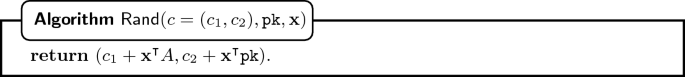
Rerandomization: :

We note that a ciphertext can be rerandomized, which is done by homomorphically adding an encryption of 0. The algorithm $\textsf {Rand}$ takes as input a cipertext and the corresponding public key, as well as a (random) vector $\mathbf {x} \in \{0,1\}^{m}$.

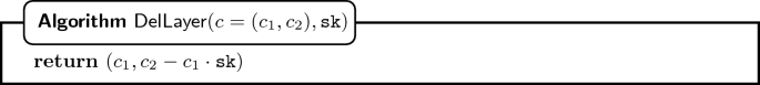
Adding and Deleting Layers of Encryption: :

Given an encryption of a bit b under the public key $\texttt {pk} = A\cdot \texttt {sk} + \mathbf {e}$, and a secret key $\texttt {sk} '$ with corresponding public key $\texttt {pk} ' = A \cdot \texttt {sk} ' + \mathbf {e}'$, one can add a layer of encryption, i.e. obtain a ciphertext under the public key . Also, one can delete a layer of encryption.

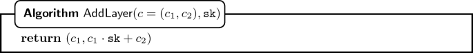
Error Analysis. Every time we add a layer, the error increases. Hence, we need to ensure that the error does not increase too much. After l steps, the error in the public key is $\texttt {pk} _{0\dots l} = \sum _{i = 0}^{l} \mathbf {e}_i$, where $\mathbf {e}_i$ is the error added in each step. The error in the ciphertext is $c_{0\dots l} = \sum _{i = 0}^{l} \mathbf {x}_{i} \sum _{j=0}^{i} \mathbf {e}_j$, where the $\mathbf {x}_{i}$ is the chosen randomness in each step. Since $\mathbf {x}_i \in \{0,1\}^{m}$, the error in the ciphertext can be bounded by $m \cdot \max _{i}\{\big |\mathbf {e}_i\big |_{\infty }\} \cdot l^2$, which is quadratic in the number of steps.

Homomorphic XOR: :

A PKCR encryption scheme requires a slightly stronger version of homomorphism. In particular, homomorphic operation includes the rerandomization of the ciphertexts. Hence, the algorithm $\textsf {hXor}$ also calls $\textsf {Rand}$. The inputs to $\textsf {hXor}$ are two ciphertexts encrypted under the same public key and the corresponding public key.

 

Appendices

Appendix

A Topology-Hiding Broadcast

This section contains supplementary material for Sect. 3.

1.1 A.1 Protocol Leaking One Bit

In this section we prove Theorem 2 from Sect. 3.1.

Theorem 2. Let $\kappa$ be the security parameter. For $\texttt {T} = 8 n^3 (\log (n) + \kappa )$ the protocol BC-OB$({ \texttt {T}},(d_i,b_i)_{P _i \in \mathcal {P}}))$ topology-hidingly realizes $\mathcal {F}_{\textsc {info}} ^{\mathcal {L}_{OB}} || \mathcal {F}_{\textsc {BC}}$ (with abort) in the $\mathcal {F}_{\textsc {net}}$ hybrid-world, where the leakage function $\mathcal {L}_{OB}$ is the one defined as above. If no crashes occur, then there is no abort and there is no leakage.

Proof

Completeness. We first show that the protocol is complete. To this end, we need to ensure that the probability that all parties get the correct output is overwhelming in $\kappa$. That is, the probability that all non-dummy random walks (of length $\texttt {T} = 8 n^3 (\log (n) + \kappa )$) reach all nodes is overwhelming.

By Lemma 1, a walk of length $8 n^3 \tau$ does not reach all nodes with probability at most $\frac{1}{2^\tau }$. Then, using the union bound, we obtain that the probability that there is a party whose walk does not reach all nodes is at most $\frac{n}{2^\tau }$. Hence, all n walks (one for each party) reach all nodes with probability at least $1-\frac{n}{2^\tau }$. If we want this value to be overwhelming, e.g. $1-\frac{1}{2^{\kappa }}$, we can set .

Soundness. We now need to show that no environment can distinguish between the real world and the simulated world, when given access to the adversarially-corrupted parties. We first describe on a high level the simulator $\mathcal {S}_{OB}$ and argue that it simulates the real execution.

In essence, the task of $\mathcal {S}_{OB}$ is to simulate the messages sent by honest parties to passively corrupted parties. Consider a corrupted party $P _c$ and its honest neighbor $P _h$. The messages sent from $P _h$ to $P _c$ during the Aggregate Stage are ciphertexts, to which $P _h$ added a layer, and corresponding public keys. Since $P _h$ is honest, the adversary does not know the secret keys corresponding to the sent public keys. Hence, $\mathcal {S}_{OB}$ can simply replace them with encryptions of a pair (1, 1) under a freshly generated public key. The group structure of keys in PKCR guarantees that a fresh key has the same distribution as the composed key (after executing $\textsf {AddLayer}$). Semantic security implies that the encrypted message can be replaced by (1, 1).

Consider now the Decrypt Stage at round r. Let ${{\texttt {pk}}_{c \rightarrow h}^{({r})}}$ be the public key sent by $P _c$ to $P _h$ in the Aggregate Stage (note that this is not the key discussed above; there we argued about keys sent in the opposite direction). $\mathcal {S}_{OB}$ will send to $P _c$ a fresh encryption under ${{\texttt {pk}}_{c \rightarrow h}^{({r})}}$. We now specify what it encrypts.

Note that the only interesting case is when the party $P _o$ receiving output is corrupted and when we are in the round r in which the (only one) random walk carrying the output enters an area of corrupted parties, containing $P _o$ (that is, when the walk with output contains from $P _h$ all the way to $P _o$ only corrupted parties). In this one message in round r the adversary learns the output of $P _o$. All other messages are simply encryptions of (1, 1).

For this one meaningful message, we consider three cases. If any party crashed in a phase preceding the current one, $\mathcal {S}_{OB}$ sends an encryption of (1, 1) (as in the real world the walk is made dummy by an unhappy party). If no crashes occurred up to this point (round r in given phase), $\mathcal {S}_{OB}$ encrypts the output received from $\mathcal {F}_{\textsc {BC}}$. If a crash happened in the given phase, $\mathcal {S}_{OB}$ queries the leakage oracle $\mathcal {L}_{OB}$, which essentially executes the protocol and tells whether the output or (1, 1) should be sent.

Simulator. Below, we present the pseudocode of the simulator. The essential part of it is the algorithm $\textsf {PhaseSimulation}$, which is also illustrated in Fig. 1.

We prove that no environment can tell whether it is interacting with $\mathcal {F}_{\textsc {net}}$ and the adversary in the real world or with $\mathcal {F}_{\textsc {info}} ^{\mathcal {L}_{}}$ and the simulator in the ideal world.

Fig. 1.

An example of the algorithm executed by the simulator $\mathcal {S}_{OB}$. The filled circles are the corrupted parties. The red line represents the random walk generated by $\mathcal {S}_{OB}$ in Step 5, in this case of length $\ell =3$. $\mathcal {S}_{OB}$ simulates the Decrypt Stage by sending fresh encryptions of (1, 1) at every round from every honest party to each of its corrupted neighbors, except in round $2\texttt {T}-3$ from $P_i$ to $P_j$. If no crash occurred up to that point, $\mathcal {S}_{OB}$ sends encryption of $(b^{out},0)$. Otherwise, it queries the leakage oracle about the walk of length $\texttt {T}-3$, starting at $P _i$.

Hybrids and Security Proof.

 

Hybrid 1. :

$\mathcal {S}_{1}$ simulates the real world exactly. This means, $\mathcal {S}$ has information on the entire topology of the graph, each party’s input, and can simulate identically the real world.

Hybrid 2. :

$\mathcal {S}_{2}$ replaces the real keys with the simulated public keys, but still knows everything about the graph as in the first hybrid. More formally, in each random walk phase and for each party $P _i \in \mathcal {P}\setminus \mathcal {Z}^p$ where $\mathbf {N}_G(P _i) \cap \mathcal {Z}^p\ne \varnothing$, $\mathcal {S}_{2}$ generates T key pairs $({{\texttt {pk}}_{i \rightarrow j}^{({1})}},{{\texttt {sk}}_{i \rightarrow j}^{({1})}})$, $\dots$, $({{\texttt {pk}}_{i \rightarrow j}^{({\texttt {T}})}},{{\texttt {sk}}_{i \rightarrow j}^{({\texttt {T}})}})$ for every neighbor $P_j \in \mathbf {N}_G(P _i) \cap \mathcal {Z}^p$. In each round r of the corresponding Aggregate Stage and for every neighbor $P _j \in \mathbf {N}_G(P _i) \cap \mathcal {Z}^p$, $\mathcal {S}_{2}$ does the following. $P_i$ receives ciphertext $[b,u]_{{{\texttt {pk}}_{* \rightarrow i}^{({r})}}}$ and the public key ${{\texttt {pk}}_{* \rightarrow i}^{({r})}}$ destined for $P _j$. Instead of adding a layer and homomorphically OR’ing the bit $b_i$, $\mathcal {S}_{2}$ computes $(b',u') = (b\vee b_i \vee u_i, u\vee u_i)$, and sends $[b',u']_{{{\texttt {pk}}_{i \rightarrow j}^{({r})}}}$ to $P _j$. In other words, it sends the same message as $\mathcal {S}_{1}$ but encrypted with a fresh public key. In the corresponding Decrypt Stage, $P _i$ will get back a ciphertext from $P _j$ encrypted under this exact fresh public key.

Hybrid 3. :

$\mathcal {S}_{3}$ now simulates the ideal functionality during the Aggregate Stage. It does so by sending encryptions of (1, 1) instead of the actual messages and unhappy bits. More formally, in each round r of the Aggregate Stage and for all parties $P _i \in \mathcal {P}\setminus \mathcal {Z}^p$ and $P_j \in \mathbf {N}_G(P _i) \cap \mathcal {Z}^p$, $\mathcal {S}_{3}$ sends $[1,1]_{{{\texttt {pk}}_{i \rightarrow j}^{({r})}}}$ instead of the ciphertext $[b,u]_{{{\texttt {pk}}_{i \rightarrow j}^{({r})}}}$ sent by $\mathcal {S}_{2}$.

Hybrid 4. :

$\mathcal {S}_{4}$ does the same as $\mathcal {S}_{OB}$ during the Decrypt Stage for all steps except for round $2\texttt {T}-\ell$ of the first random walk phase in which the adversary crashes a party. This corresponds to the original description of the simulator except for the ‘Otherwise’ condition of Step 6 in the Decrypt Stage.

Hybrid 5. :

$\mathcal {S}_{5}$ is the actual simulator $\mathcal {S}_{OB}$.

 

In order to prove that no environment can distinguish between the real world and the ideal world, we prove that no environment can distinguish between any two consecutive hybrids when given access to the adversarially-corrupted nodes.

Claim 1

No efficient distinguisher D can distinguish between Hybrid 1 and Hybrid 2.

Proof: The two hybrids only differ in the computation of the public keys that are used to encrypt messages in the Aggregate Stage from any honest party $P _i \in \mathcal {P}\setminus \mathcal {Z}^p$ to any dishonest neighbor $P _j \in \mathbf {N}_G(P _i) \cap \mathcal {Z}^p$.

In Hybrid 1, party $P _i$ sends to $P _j$ an encryption under a fresh public key in the first round. In the following rounds, the encryption is sent either under a product key ${{\overline{\texttt {pk}}}_{i \rightarrow j}^{({r})}} = {{\overline{\texttt {pk}}}_{k \rightarrow i}^{({r-1})}} \circledast {{\texttt {pk}}_{i \rightarrow j}^{({r})}}$ or under a fresh public key (if $P _i$ is unhappy). Note that ${{\overline{\texttt {pk}}}_{k \rightarrow i}^{({r-1})}}$ is the key $P _i$ received from a neighbor $P _k$ in the previous round.

In Hybrid 2, party $P _i$ sends to $P _j$ an encryption under a fresh public key ${{\texttt {pk}}_{i \rightarrow j}^{({r})}}$ in every round.

The distribution of the product key used in Hybrid 1 is the same as the distribution of a freshly generated public-key. This is due to the (fresh) ${{\texttt {pk}}_{i \rightarrow j}^{({r})}}$ key which randomizes the product key. Therefore, no distinguisher can distinguish between Hybrid 1 and Hybrid 2.                                                           $\blacksquare$

Claim 2

No efficient distinguisher D can distinguish between Hybrid 2 and Hybrid 3.

Proof: The two hybrids differ only in the content of the encrypted messages that are sent in the Aggregate Stage from any honest party $P _i \in \mathcal {P}\setminus \mathcal {Z}^p$ to any dishonest neighbor $P _j \in \mathbf {N}_G(P _i) \cap \mathcal {Z}^p$.

In Hybrid 2, party $P _i$ sends to $P _j$ in the first round an encryption of $(b_i \vee u_i,u_i)$. In the following rounds, $P _i$ sends to $P _j$ either an encryption of $(b\vee b_i \vee u_i, u\vee u_i)$, if message $(b,u)$ is received from neighbor $\pi _i^{-1}(j)$, or an encryption of (1, 1) if no message is received.

In Hybrid 3, all encryptions that are sent from party $P _i$ to party $P _j$ are replaced by encryptions of (1, 1).

Since the simulator chooses a key independent of any key chosen by parties in $\mathcal {Z}^p$ in each round, the key is unknown to the adversary. Hence, the semantic security of the encryption scheme guarantees that the distinguisher cannot distinguish between both encryptions. $\blacksquare$

Claim 3

No efficient distinguisher D can distinguish between Hybrid 3 and Hybrid 4.

Proof: The only difference between the two hybrids is in the Decrypt Stage. We differentiate two cases:

• A phase where the adversary did not crash any party in this or any previous phase. In this case, the simulator $\mathcal {S}_{3}$ sends an encryption of $(b_{W},u_{W})$, where $b_{W} = \bigvee _{P _j \in W} b_j$ is the OR of all input bits in the walk and $u_{W} = 0$, since no crash occurred. $\mathcal {S}_{4}$ sends an encryption of $(b^{out},0)$, where $b^{out} = \bigvee _{P _i \in \mathcal {P}} b_i$. Since the graph is connected, $b^{out} = b_{W}$ with overwhelming probability, as proven in Corollary 1. Also, the encryption in Hybrid 4 is done with a fresh public key which is indistinguishable with the encryption done in Hybrid 3 by OR’ing many times in the graph, as shown in Claim 2.1 in [ALM17a].

• A phase where the adversary crashed a party in a previous phase or any round different than $2\texttt {T}-\ell$ of the first phase where the adversary crashes a party. In Hybrid 4 the parties send an encryption of (1, 1). This is also the case in Hybrid 3, because even if a crashed party disconnected the graph, each connected component contains a neighbor of a crashed party. Moreover, in Hybrid 4, the messages are encrypted with a fresh public key, and in Hybrid 3, the encryptions are obtained by the homomorphic OR operation. Both encryptions are indistinguishable, as shown in Claim 2.1 in [ALM17a].       $\blacksquare$

Claim 4

No efficient distinguisher D can distinguish between Hybrid 4 and Hybrid 5.

Proof: The only difference between the two hybrids is in the Decrypt Stage, at round $2\texttt {T}-\ell$ of the first phase where the adversary crashes.

Let F be the set of pairs $(P _f,r)$ such that $\mathcal {A}$ crashed $P _f$ at round r of the phase. In Hybrid 4, a walk W of length $\texttt {T}$ is generated from party $P _o$. Let $W_1$ be the region of W from $P _o$ to the first not passively corrupted party and let $W_2$ be the rest of the walk. Then, the adversary’s view at this step is the encryption of (1, 1) if one of the crashed parties breaks $W_2$, and otherwise an encryption of $(b_{W},0)$. In both cases, the message is encrypted under a public key for which the adversary knows the secret key.

In Hybrid 5, a walk $W_1'$ is generated from $P _o$ of length $\ell \le \texttt {T}$ ending at the first not passively corrupted party $P _i$. Then, the simulator queries the leakage function on input $(F,P _i,\texttt {T}-\ell )$, which generates a walk $W_2'$ of length $\texttt {T}-\ell$ from $P _i$, and checks whether $W_2'$ is broken by any party in F. If $W_2'$ is broken, $P _i$ sends an encryption of (1, 1), and otherwise an encryption of $(b_{W},0)$. Since the walk $W'$ defined as $W_1'$ followed by $W_2'$ follows the same distribution as W, $b_{W} = b^{out}$ with overwhelming probability, and the encryption with a fresh public key which is indistinguishable with the encryption done by OR’ing many times in the graph, then it is impossible to distinguish between Hybrid 4 and Hybrid 5.       $\blacksquare$

This concludes the proof of soundness.    $\square$

1.2 A.2 Protocol Leaking a Fraction of a Bit

In this section, we give a formal description of the random-walk phase protocol $\textsf {ProbabilisticRandomWalkPhase} _{p}$ for the broadcast protocol $\textsf {BC-FB} _{p}$ from Sect. 3.2. Note that this protocol should be repeated $\rho$ times in the actual protocol. The boxes indicate the parts where it differs from the random-walk phase protocol $\textsf {RandomWalkPhase}$ for the broadcast protocol leaking one bit (cf. Sect. 3.1).

Security Proof of the Protocol Leaking a Fraction of a Bit.

In this section we prove Theorem 3 from Sect. 3.2.

Theorem 3. Let $\kappa$ be the security parameter. For $\tau = \log (n) + \kappa$, T $= 8 n^3 \tau$ and $\rho = \tau / (p' - 2^{-\tau })$, where $p' = 1 / \lfloor 1/p \rfloor$, the protocol BC-FB $_p$ (T, $\rho ,(d_i,b_i)_{P _i \in \mathcal {P}}))$ topology-hidingly realizes $\mathcal {F}_{\textsc {info}} ^{\mathcal {L}_{FB_p}} || \mathcal {F}_{\textsc {BC}}$ (with abort) in the $\mathcal {F}_{\textsc {net}}$ hybrid-world, where the leakage function $\mathcal {L}_{FB_p}$ is the one defined as above. If no crashes occur, then there is no abort and there is no leakage.

Proof

Completeness. We first show that the protocol is complete. That is, that if the adversary does not crash any party, then every party gets the correct output (the OR of all input bits) with overwhelming probability. More specifically, we show that if no crashes occur, then after $\rho$ repetitions of a phase, the party $P _o$ outputs the correct value with probability at least $1 - 2^{-(\kappa +\log (n))}$. The overall completeness follows from the union bound: the probability that all n parties output the correct value is at least $1-2^{-\kappa }$.

Notice that if the output of any of the $\rho$ repetitions intended for $P _o$ is correct, then the overall output of $P _o$ is correct. A given repetition can only give an incorrect output when either the random walk does not reach all parties, which happens with probability at most $2^{-\tau }$, or when the repetition fails, which happens with probability $1-p'$. Hence, the probability that a repetition gives the incorrect result is at most $1-p'+2^{-\tau }$. The probability that all repetitions are incorrect is then at most $(1-p'+2^{-\tau })^\rho \le 2^{-(\kappa +\log (n))}$ (the inequality holds for $0 \le p'-2^{-\tau } \le 1$).

Soundness. We show that no environment can distinguish between the real world and the simulated world, when given access to the adversarially-corrupted nodes. The simulator $\mathcal {S}_{FB}$ for $\textsf {BC-FB} _{p}$ is a modification of $\mathcal {S}_{OB}$. Here we only sketch the changes and argue why $\mathcal {S}_{FB}$ simulates the real world.

In each of the $\rho$ repetitions of a phase, $\mathcal {S}_{FB}$ executes a protocol very similar to the one for $\mathcal {S}_{OB}$. In the Aggregate Stage, $\mathcal {S}_{FB}$ proceeds almost identically to $\mathcal {S}_{OB}$ (except that it sends encryptions of vectors $(1,\dots ,1)$ instead of only two values). In the Decrypt Stage the only difference between $\mathcal {S}_{FB}$ and $\mathcal {S}_{OB}$ is in computing the output for the party $P _o$ (as already discussed in the proof of Theorem 2, $\mathcal {S}_{FB}$ does this only when $P _o$ is corrupted and the walk carrying the output enters an area of corrupted parties). In the case when there were no crashes before or during given repetition of a phase, $\mathcal {S}_{OB}$ would simply send the encrypted output. On the other hand, $\mathcal {S}_{FB}$ samples a value from the Bernoulli distribution with parameter p and sends the encrypted output only with probability p, while with probability $1-p$ it sends the encryption of (1, 0). Otherwise, the simulation is the same as for $\mathcal {S}_{OB}$.

It can be easily seen that $\mathcal {S}_{FB}$ simulates the real world in the Aggregate Stage and in the Decrypt Stage in every message other than the one encrypting the output. But even this message comes from the same distribution as the corresponding message sent in the real world. This is because in the real world, if the walk was not broken by a crash, this message contains the output with probability p. The simulator encrypts the output also with probability p in the two possible cases: when there was no crash ($\mathcal {S}_{FB}$ samples from the Bernoulli distribution) and when there was a crash but the walk was not broken ($\mathcal {L}_{FB}$ is defined in this way).

Simulator. The simulator $\mathcal {S}_{FB}$ proceeds almost identically to the simulator $\mathcal {S}_{OB}$ given in the proof of Theorem 2 (cf. Sect. A.1). We only change the algorithm $\textsf {PhaseSimulation}$ to $\textsf {ProbabilisticPhaseSimulation}$ and execute it $\rho$ times instead of only once.

Hybrids and Security Proof. We consider similar steps as the hybrids from Sect. A.1.

 

Hybrid 1. :

$\mathcal {S}_{1}$ simulates the real world exactly. This means, $\mathcal {S}_{1}$ has information on the entire topology of the graph, each party’s input, and can simulate identically the real world.

Hybrid 2. :

$\mathcal {S}_{2}$ replaces the real keys with the simulated public keys, but still knows everything about the graph as in the first hybrid. More formally, in each subphase of each random walk phase and for each party $P _i \in \mathcal {P}\setminus \mathcal {Z}^p$ where $\mathbf {N}_G(P _i) \cap \mathcal {Z}^p\ne \varnothing$, $\mathcal {S}_{2}$ generates T key pairs $({{\texttt {pk}}_{i \rightarrow j}^{({1})}},{{\texttt {sk}}_{i \rightarrow j}^{({1})}}), \dots , ({{\texttt {pk}}_{i \rightarrow j}^{({\texttt {T}})}},{{\texttt {sk}}_{i \rightarrow j}^{({\texttt {T}})}})$ for every neighbor $P_j \in \mathbf {N}_G(P _i) \cap \mathcal {Z}^p$. Let . In each round r of the corresponding Aggregate Stage and for every neighbor $P _j \in \mathbf {N}_G(P _i) \cap \mathcal {Z}^p$, $\mathcal {S}_{2}$ does the following: $P_i$ receives ciphertext $[b_1,\dots ,b_{\alpha },u]_{{{\texttt {pk}}_{* \rightarrow i}^{({r})}}}$ and the public key ${{\texttt {pk}}_{* \rightarrow i}^{({r})}}$ destined for $P _j$. Instead of adding a layer and homomorphically OR’ing the bit $b_i$, $\mathcal {S}_{2}$ computes $(b'_1,\dots ,b'_{\alpha }, u') = (b_1 \vee b_i \vee u_i, \cdots , b_\alpha \vee b_i \vee u_i, u\vee u_i)$, and sends $[b'_{\sigma (1)},\cdots , b'_{\sigma (\alpha )}, u']_{{{\texttt {pk}}_{i \rightarrow j}^{({r})}}}$ to $P _j$, where $\sigma$ is a random permutation on $\alpha$ elements. In other words, it sends the same message as $\mathcal {S}_{1}$ but encrypted with a fresh public key. In the corresponding Decrypt Stage, $P _i$ will get back a ciphertext from $P _j$ encrypted under this exact fresh public key.

Hybrid 3. :

$\mathcal {S}_{3}$ now simulates the ideal functionality during the Aggregate Stage. It does so by sending encryptions of $(1,\dots ,1)$ instead of the actual messages and unhappy bits. More formally, let . In each round r of a subphase of a random walk phase and for all parties $P _i \in \mathcal {P}\setminus \mathcal {Z}^p$ and $P_j \in \mathbf {N}_G(P _i) \cap \mathcal {Z}^p$, $\mathcal {S}_{3}$ sends $[1,1,\dots ,1]_{{{\texttt {pk}}_{i \rightarrow j}^{({r})}}}$ instead of the ciphertext $[b_1,\dots ,b_{\alpha },u]_{{{\texttt {pk}}_{i \rightarrow j}^{({r})}}}$ sent by $\mathcal {S}_{2}$.

Hybrid 4. :

$\mathcal {S}_{4}$ does the same as $\mathcal {S}_{FB}$ during the Decrypt Stage for all phases and subphases except for the first subphase of a random walk phase in which the adversary crashes a party.

Hybrid 5. :

$\mathcal {S}_{5}$ is the actual simulator $\mathcal {S}_{FB}$.

  The proofs that no efficient distinguisher D can distinguish between Hybrid 1, Hybrid 2 and Hybrid 3 are similar to the Claims 1 and 2. Hence, we prove indistinguishability between Hybrid 3, Hybrid 4 and Hybrid 5.

Claim 5

No efficient distinguisher D can distinguish between Hybrid 3 and Hybrid 4.

Proof: The only difference between the two hybrids is in the Decrypt Stage. We differentiate three cases:

• A subphase l of a phase k where the adversary did not crash any party in this phase, any previous subphase, or any previous phase. In this case, $\mathcal {S}_{3}$ sends with probability p an encryption of $(b_{W},u_{W})$, where $b_{W} = \bigvee _{u \in W} b_u$ is the OR of all input bits in the walk and $u_{W} = 0$ (since no crash occurs), and with probability $1-p$ an encryption of (1, 0). On the other hand, $\mathcal {S}_{4}$ samples r from a Bernoulli distribution with parameter p, and if $r = 1$, it sends an encryption of $(b_{out},0)$, where $b_{out} = \bigvee _{i \in [n]} b_i$, and if $r=0$ it sends an encryption of (1, 0). Since the graph is connected, $b_{out} = b_{W}$ with overwhelming probability, as proven in Corollary 1. Also, the encryption in Hybrid 4 is done with a fresh public key which is indistinguishable with the encryption done in Hybrid 3 by OR’ing many times in the graph, as shown in Claim 2.1. in [ALM17a].

• A subphase l of a phase k where the adversary crashed a party in a previous subphase or a previous phase. In Hybrid 3 the parties send encryptions of (1, 1). This is also the case in Hybrid 4, because even if a crashed party disconnected the graph, each connected component contains a neighbor of a crashed party. Moreover, in Hybrid 4, the messages are encrypted with a fresh public key, and in Hybrid 3, the encryptions are obtained by the homomorphic OR operation. Both encryptions are indistinguishable, as shown in Claim 2.1. in [ALM17a].

$\blacksquare$

Claim 6

No efficient distinguisher D can distinguish between Hybrid 4 and Hybrid 5.

Proof: The only difference between the two hybrids is in the Decrypt Stage of the first subphase of a phase where the adversary crashes.

Let F be the set of pairs $(P _f,r)$ such that $\mathcal {A}$ crashed $P _f$ at round r of the phase. In Hybrid 4, a walk W of length $\texttt {T}$ is generated from party $P _o$. Let $W_1$ be the region of W from $P _o$ to the first not passively corrupted party and let $W_2$ be the rest of the walk. Then, the adversary’s view at this step is the encryption of (1, 1) if one of the crashed parties breaks $W_2$ or if the walk became dummy (which happens with probability $1-p$, since the ciphertexts are permuted randomly and only one ciphertext out of $\frac{1}{p}$ contains $b_{W}$). Otherwise, the adversary’s view is an encryption of $(b_{W},0)$. In both cases, the message is encrypted under a public key for which the adversary knows the secret key.

In Hybrid 5, a walk $W_1'$ is generated from $P _o$ of length $\ell \le \texttt {T}$ ending at the first not passively corrupted party $P _i$. Then, the simulator queries the leakage function on input $(F,P _i,\texttt {T}-\ell )$. Then, with probability p it generates a walk $W_2'$ of length $\texttt {T}-\ell$ from $P _i$, and checks whether $W_2'$ is broken by any party in F. If $W_2'$ is broken, $P _i$ sends an encryption of (1, 1), and otherwise an encryption of $(b_{W},0)$. Since the walk $W'$ defined as $W_1'$ followed by $W_2'$ follows the same distribution as W, $b_{W} = b^{out}$ with overwhelming probability, and the encryption with a fresh public key which is indistinguishable with the encryption done by OR’ing many times in the graph, then it is impossible to distinguish between Hybrid 4 and Hybrid 5.       $\blacksquare$

This concludes the proof of soundness.    $\square$

References

Asharov, G., Jain, A., López-Alt, A., Tromer, E., Vaikuntanathan, V., Wichs, D.: Multiparty computation with low communication, computation and interaction via threshold FHE. In: Pointcheval, D., Johansson, T. (eds.) EUROCRYPT 2012. LNCS, vol. 7237, pp. 483–501. Springer, Heidelberg (2012). https://doi.org/10.1007/978-3-642-29011-4_29
Akavia, A., LaVigne, R., Moran, T.: Topology-hiding computation on all graphs. In: Katz, J., Shacham, H. (eds.) CRYPTO 2017. LNCS, vol. 10401, pp. 447–467. Springer, Cham (2017). https://doi.org/10.1007/978-3-319-63688-7_15
Akavia, A., LaVigne, R., Moran, T.: Topology-hiding computation on all graphs. Cryptology ePrint Archive, Report 2017/296 (2017). http://eprint.iacr.org/2017/296
Akavia, A., Moran, T.: Topology-hiding computation beyond logarithmic diameter. In: Coron, J.-S., Nielsen, J.B. (eds.) EUROCRYPT 2017. LNCS, vol. 10212, pp. 609–637. Springer, Cham (2017). https://doi.org/10.1007/978-3-319-56617-7_21
Ball, M., Boyle, E., Malkin, T., Moran, T.: Exploring the boundaries of topology-hiding computation. In: Nielsen, J.B., Rijmen, V. (eds.) EUROCRYPT 2018. LNCS, vol. 10822, pp. 294–325. Springer, Cham (2018). https://doi.org/10.1007/978-3-319-78372-7_10
Bos, J., den Boer, B.: Detection of disrupters in the DC protocol. In: Quisquater, J.-J., Vandewalle, J. (eds.) EUROCRYPT 1989. LNCS, vol. 434, pp. 320–327. Springer, Heidelberg (1990). https://doi.org/10.1007/3-540-46885-4_33
Chaum, D.L.: Untraceable electronic mail, return addresses, and digital pseudonyms. Commun. ACM 24(2), 84–90 (1981)
Chaum, D.: The dining cryptographers problem: unconditional sender and recipient untraceability. J. Cryptol. 1(1), 65–75 (1988)
Canetti, R., Lin, H., Tessaro, S., Vaikuntanathan, V.: Obfuscation of probabilistic circuits and applications. In: Dodis, Y., Nielsen, J.B. (eds.) TCC 2015. LNCS, vol. 9015, pp. 468–497. Springer, Heidelberg (2015). https://doi.org/10.1007/978-3-662-46497-7_19
Checkoway, S., et al.: On the practical exploitability of dual EC in TLS implementations. In: USENIX Security Symposium, pp. 319–335 (2014)
Dolev, D., Dwork, C., Waarts, O., Yung, M.: Perfectly secure message transmission. In: 31st FOCS, pp. 36–45. IEEE Computer Society Press, October 1990
Golle, P., Juels, A.: Dining cryptographers revisited. In: Cachin, C., Camenisch, J.L. (eds.) EUROCRYPT 2004. LNCS, vol. 3027, pp. 456–473. Springer, Heidelberg (2004). https://doi.org/10.1007/978-3-540-24676-3_27
Heninger, N., Durumeric, Z., Wustrow, E., Halderman, J.A.: Mining your PS and QS: detection of widespread weak keys in network devices. In: USENIX Security Symposium, vol. 8, p. 1 (2012)
Hinkelmann, M., Jakoby, A.: Communications in unknown networks: preserving the secret of topology. Theoret. Comput. Sci. 384(2–3), 184–200 (2007)
Hirt, M., Maurer, U., Tschudi, D., Zikas, V.: Network-hiding communication and applications to multi-party protocols. In: Robshaw, M., Katz, J. (eds.) CRYPTO 2016. LNCS, vol. 9815, pp. 335–365. Springer, Heidelberg (2016). https://doi.org/10.1007/978-3-662-53008-5_12
Lavigne, R., Liu-Zhang, C.-D., Maurer, U., Moran, T., Mularczyk, M., Tschudi, D.: Topology-hiding computation beyond semi-honest adversaries. Cryptology ePrint Archive, Report 2018/255 (2018). https://eprint.iacr.org/2018/255
Moran, T., Orlov, I., Richelson, S.: Topology-hiding computation. In: Dodis, Y., Nielsen, J.B. (eds.) TCC 2015. LNCS, vol. 9014, pp. 159–181. Springer, Heidelberg (2015). https://doi.org/10.1007/978-3-662-46494-6_8
Reiter, M.K., Crowds, R.A.: Anonymity for web transaction. ACM Trans. Inf. Syst. Secur. 1(1), 66–92 (1988)
Regev, O.: On lattices, learning with errors, random linear codes, and cryptography. J. ACM (JACM) 56(6), 34 (2009)
Syverson, P.F., Goldschlag, D.M., Reed, M.G.: Anonymous connections and onion routing. In: 1997 Proceedings of IEEE Symposium on Security and Privacy, pp. 44–54. IEEE (1997)
Author information
Authors and Affiliations
Corresponding author
Editor information
Editors and Affiliations