Modelling and Optimisation of a RoboCup MSL Coilgun

Abstract

This paper focuses on the modelling and optimization of a RoboCup Middle Size League (MSL) coil-gun. A mechatronic model coupling electrical, mechanical and electromagnetic models is proposed. This model is used for optimizing an indirect coil-gun used on limited size robots at the RoboCup for kicking real soccer balls. Applied to a well defined existing coil gun [6], we show that optimizing the initial position of the plunger and the length of a plunger extension leads to increase the ball speed by $30\%$ compared to the results presented in a previous study.

1 Introduction

An electromagnetic launcher (EML) is a system using electricity for propelling a projectile [5]. A coil gun is a type of EML, having only the ability to launch magnetic objects (such as iron rods) by converting electrical energy into kinetic energy using a coil [1].

Launching non-magnetic objects cannot be done directly using coil guns because they are not affected by magnetic field but can be done using an “indirect coil gun”, having a magnetic plunger accelerated by a coil, propelling an non-magnetic object by continuous contact or elastic shock. Both these propelling techniques can be combined in a multi-phase EML. Optimization of this type of launcher is the purpose of this work.

Optimizing limited size indirect coil guns is the scope of this paper. For illustrating our purpose, we have chosen to optimize a kicking system used at the RoboCup in Middle Size League, which is a competition of robot playing soccer and having a limited size and weight for embedding soccer balls launching systems. This article is divided into three parts:

• In Sect. 2, principles of coil guns are presented with limitations concerning their modelling.

• In Sect. 3, a mechanic and electromagnetic model is proposed and implemented using finite elements simulation tools for the electromagnetic part of the coil gun, and using Matlab Simulink for the mechanical and electrical aspects.

• In Sect. 4, simulation results are discussed in order to optimize the parameters of an existing indirect coil gun.

RoboCup is an international competition of robot teams playing soccer with a goal: winning against a soccer professional team by 2050. In Middle Size League (MSL), teams are composed of 5 robots playing autonomously on a 22 m by 14 m soccer field with a real soccer ball (diameter 22 cm) weighting 450 g. Each robot have a maximum length of 52 cm, a maximum width of 52 cm and a maximum height of 80 cm. Current kicking systems used in MSL have the ability of propelling balls with a speed of $12\,{\text {m.s}}^{-1}$. This speed is interesting and allows to kick balls at a distance of 15 m but is limited compared with real soccer players. In order to make a comparison, a shoot from a professional soccer player can reach $130\,{\text {km.h}}^{-1}$, compared with $43\,{\text {km.h}}^{-1}$ for current MSL robots. In terms of kinetic energy, $E_K = \frac{1}{2}\,{\text {mv}}^2 = 32$ J is transmitted to the ball at the RoboCup, compared to $E_K = 300$ J transmitted by a real professional player. The ratio is about 10 times, showing that an important step has to be done in order to compete with humans.

Fig. 1.

Kicking system in a RoboCup robot

RoboCup MSL case study has been chosen due to the relevancy of trade-off consisting in an optimization of the speed of a ball kicked by an indirect coil gun, while having strong size constraints due to competition rules. RoboCup robots need compact but powerful coil guns. Existing systems able to strike a ball at $12\,{\text {m.s}}^-1$ have an acceleration of about $100\,\mathrm{G}$ and a strike time of about 20 ms. As shown in Fig. 1, the size of the whole kicking system, including the indirect coil gun, is about 30 cm including the coil and the iron rod, with a coil size of about 10 cm to 12 cm in length, a rod size of about 13 cm in length, and a rod stroke of about 12 cm.

2 Principles of Coil Guns

2.1 Physical Concept

Coil guns are made using a variable reluctance magnetic circuit composed of a fixed magnetic circuit looped by an magnetic iron projectile. A coil is placed around the stroke of the iron rod in order to magnetize the magnetic circuit and to create a magnetic force on the rod.

Considering that the magnetic field in a magnetic circuit tends to be maximized if possible, the air gap in a magnetic circuit tends to be reduced, resulting in a force on the rod propelling it when the magnetic circuit is excited with a coil crossed by a current pulse as shown in Fig. 2. This is the principle of a variable reluctance actuator.

Fig. 2.

Coil gun principle

In our case study, a large capacitor ($4700\,{\upmu }\mathrm{F}$) is discharged in the coil in order to produce a high current generating the magnetic field and force. A mobile plunger (iron rod) is able to move in this field, sliding in a stainless steel tube. Iron rod is attracted to the centre of the stainless steel tube and thus accelerated until it reaches this point. It can be slowed down if the plunger goes over this point while the current in the coil is still present, but this doesn’t happens in real conditions as shown later.

Current discharge on the coil can be described by a second order RLC differential equation, but having non-constant coefficients because of the changing value of the inductor over the time. In this paper, we propose an electrical model taking into account the variation of the inductance when the iron rod slides forward in the coil.

2.2 Electromagnetic Theory and Simulation Software

Hopkinson law is the base a variable reluctance actuators: $\mathscr {F} = NI = R \varPhi$, with:

• $\mathscr {F}$: magnetomotive force (MMF and the unit is ampere-turn: At)

• N: number of turns of the coil

• I: intensity in the coil (A)

• R: reluctance ($H^{-1}$)

• $\varPhi$: flux (Wb)

Consequently, magnetic flux is equal to: $\varPhi = \dfrac{NI}{R}$ and coil force is equal to: $\overrightarrow{F} = \overrightarrow{grad}(\overrightarrow{M}\cdot \overrightarrow{B})$ with $\overrightarrow{M}=IS \overrightarrow{n}$.

Going deeper into a theoretical electrical model is interesting if the reluctance is constant, in order to find an analytical solution. However, there are 2 main factors making it non-constant: the first one is the position of the plunger, and the second one is the saturation of the magnetic circuit as shown in Fig. 3, which can be very important if the coil current is high. In order to take these non-linearities into account, a finite-element model based simulator is used for calculating the force and the inductance values under different conditions [4]. Open source software used is FEMM 4.2, programmed by D.C. Meeker.

FEMM 4.2 approximates the values of $\overrightarrow{B}$ at any place of the system for each plunger and current combination. Numerical computation is performed in a static way, meaning that the kicking system evolution can be considered as a succession of short time independent magneto-static problems. For each of these problems, following equations link magnetic field intensity B and magnetic excitation H:

$$\begin{aligned} \nabla \cdot \overrightarrow{B}=0 \end{aligned}$$

(1)

$$\begin{aligned} \nabla \times \overrightarrow{H}=J \end{aligned}$$

(2)

$\overrightarrow{B}$ and $\overrightarrow{H}$ can be linked together in a linear approach:

$$\begin{aligned} \overrightarrow{B}=\mu \overrightarrow{H} \end{aligned}$$

(3)

or in a more realistic non-linear approach:

$$\begin{aligned} \overrightarrow{B}=\mu (\overrightarrow{H})\overrightarrow{H} \end{aligned}$$

(4)

Fig. 3.

Magnetic field saturation in iron

Fig. 4.

FEMM 4.2 simulation with the plunger outside the coil

FEMM software tries to find a field that satisfies the linear approach and the flux density equation with the magnetic vector potential $\overrightarrow{A}$ defined as:

$$\begin{aligned} \overrightarrow{B}=\nabla \times \overrightarrow{A} \end{aligned}$$

(5)

$\overrightarrow{A}$ can be found by the software using Eq. 4 with a conjugate gradient method, so we can rewrite Eq. 2 as:

$$\begin{aligned} \nabla \times \left( \dfrac{1}{\mu (\overrightarrow{H})}\nabla \times \overrightarrow{A}) \right) =J \end{aligned}$$

(6)

Using this equation, the software calculates $\overrightarrow{A}$ $\overrightarrow{B}$ in every place of the EML as shown on Fig. 4. It also evaluates integral values on a specific part of the system such as the inductance of the coil or the force applied on the iron plunger.

2.3 Electrical Model

The coil gun inductance L is powered by a pre-loaded high value and voltage (i.e. $4700\,{\upmu }\mathrm{F}$, $450\,\mathrm{V}$) capacitor C, switched by an Insulated Gate Bipolar Transistor (IGBT) has shown in Fig. 5. Resistor R has to be taken into account considering the high number of loops of the coil. This leads to the differential equation 7.

Fig. 5.

Electric circuit

$$\begin{aligned} \frac{d^2 U_C}{dt^2} + \frac{R}{L}\frac{dU_C}{dt} + \frac{U_C}{LC} = 0 \end{aligned}$$

(7)

This equation can be solved easily when L, C and R are constants, but L is not constant in our case. As shown in Fig. 6, simulations on FEMM 4.2 using a LUA script shows that L inductance value can vary by a factor 18 in our studying case, going from 19 mH to 342 mH for the same coil depending on the plunger position and on the coil current.

When the plunger is outside the coil and when the current is high, the inductance has the lowest values. When the plunger is at the centre of the coil and when current is low, magnetic field is well guided and magnetic materials are not saturated, leading to a high inductance value.

Fig. 6.

Variation of the inductance value depending on the plunger position and the coil current

2.4 Mechanical Model

As explained before, force on the plunger cannot be calculated analytically. Simulations using FEMM 4.2 combined with a LUA script shows (Fig. 7) that force varies in our case study from 0 to $850\,\mathrm{N}$ for the same coil depending on the plunger position and on the coil current.

Fig. 7.

Variation of the force on the plunger depending on its position and the coil current

When the plunger is outside the coil, the force is very small due to the size of the air gap which is too important. When the plunger is exactly at the centre of the coil, force is null for any value of the current because air gap is minimal. The maximal force strength is obtained for high currents and plunger positions between 40 mm and 80 mm from the centre of the coil.

3 Mixed Electrical and Mechanical Model of the Indirect Coil Gun

Inductance and magnetic force values are necessary to build a model of the coil gun for simulating it precisely. Calculated using FEMM 4.2, they are implemented using look-up tables taking into account plunger position and coil current in order to approximate inductance and force for every configurations of the system.

For this mechatronic model combining mechanic, electric and magnetic modelling, Matlab Simulink tool has been used as shown in Fig. 8.

Fig. 8.

Mechatronic model of the coil gun

3.1 Electrical Model

The electrical part is described at Fig. 9. It implements the electrical differential equation 7 using discrete blocks. This is necessary because coefficients of the equation are not constant due to the dependence of inductance L to the current and the position of the plunger.

As said before, this dependence is modelled using a look-up table (LUT) interpolating linearly the value of L using the simulations performed with FEMM 4.2.

3.2 Mechanical Model

The indirect coil gun mechanical system used for kicking balls is described at Fig. 10.

This model is not simple because as shown in Fig. 10, plunger hits a rotating aluminium bar near its centre, in order to transmit movement to the ball. Thus, movement can be split in 3 phases as shown in Fig. 11:

Fig. 9.

Electrical part of the coil gun model, including a look-up table obtained with FEMM 4.2

Fig. 10.

Simulated kicking system

Fig. 11.

Plunger speed in $m.s^{-1}$ over the time in s

• Phase 1: the plunger is accelerated without contact on the rotating bar. Acceleration is due to the magnetic force only as shown in Eq. 8. Force $F_{magneto}$ is a function of plunger position and current I. Again, this dependence is modelled using a look-up table (LUT) interpolating linearly the value of F using the simulations performed with FEMM 4.2.

  $$\begin{aligned} m_p\ddot{x} = F_{Magneto}(x, I) \end{aligned}$$

  (8)

• Phase 2: an elastic shock happens when plunger hits the rotating bar. We assume that kinetic energy is conserved as described in Eq. 9, even if for a few milliseconds a part of this one is absorbed by the ball and then given back before the ball is kicked. In theory, speeds of ball, bar and plunger are not similar after the shock, but in reality they are all moving together thanks to the deformation of the ball which ensure that the contact is permanent after the shock as shown in the slow motion picture in Fig. 12.

  $$\begin{aligned} \frac{1}{2}m_p\dot{x_{Init}}^2 = \frac{1}{2}m_p\dot{x_{Final}}^2 + \frac{1}{2}m_B\frac{R_2^2}{R_1^2}\dot{x_{Final}}^2 + \frac{1}{2}J \frac{\dot{x_{Final}}^2}{R_1^2} \end{aligned}$$

  (9)

  This leads to a plunger speed just after the shock equal to the $x_{final}$ given in Eq. 10.

  $$\begin{aligned} \dot{x_{Final}} = \sqrt{ \displaystyle \frac{m_p}{m_p+m_B\displaystyle \frac{R_2^2}{R_1^2} + \frac{J}{R_1^2}} }\dot{x_{Init}} \end{aligned}$$

  (10)

  Fig. 12.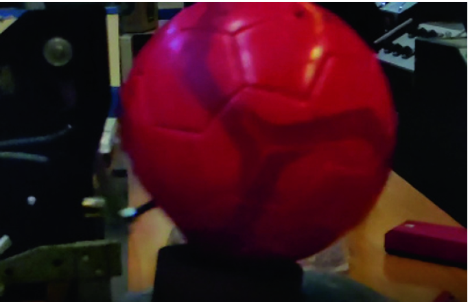

  

  Ball deformation after phase 2

• Phase 3: plunger is accelerated in contact with the rotating bar, which one is also in contact with the ball. This means that the bar applies a force on the plunger in subtraction of the magnetic force as shown in Eq. 11. This force is an inertial one due to the acceleration of the ball and the bar as shown in Eq. 12.

  $$\begin{aligned} m_p\ddot{x} = F_{Magneto}(x, I)-F_{Bar} \end{aligned}$$

  (11)

  where

  $$\begin{aligned} F_{Bar} = \frac{J_{Bar}+m_BR_2^2}{R_1}\ddot{\theta } \qquad \quad with: J_{Bar}=\dfrac{m_{Bar}R_2^2}{3} \end{aligned}$$

  (12)

  For small $\theta$ angles, $\ddot{\theta } \simeq \displaystyle \frac{\ddot{x} }{R_1}$, this leads to:

  $$\begin{aligned} \frac{m_pR_1^2+J+m_BR_2^2}{R_1^2}\ddot{x} = F_{Magneto}(x, I) \end{aligned}$$

  (13)

This mechanical model is implemented with Matlab Simulink using discrete blocks and switches for simulating the different phases of the movement (Fig. 13).

Fig. 13.

Mechanical part of the coil gun model

4 Indirect Coil Gun Simulation Results

The indirect coil gun system presented before and used in robots at the RoboCup has been simulated using Matlab Simulink. Even if the mechanical structure and the electromagnetic properties of the kicking system have been completely defined as in Fig. 10, there are 2 remaining degrees of freedom in order to optimize its power: the initial position $x_{init}$ of the plunger, and the length $L_{ext}$ of the non-magnetic extension of the plunger.

In order to compare results with other previous studies, the kicking system simulated is Tech United Team one described in [6]. Parameters of the model are the following ones:

• Distance from rotating bar axis to plunger touch point: $R_1 = 13$ cm

• Distance from rotating bar axis to ball touch point: $R_2 = 24$ cm

• Coil length: $L_{Coil} = 11.5$ cm

• Coil number of turns: $N_{Coil} = 1050$ turns

• Plunger iron rod diameter: $D_{Plunger} = 25$ mm

• Plunger iron rod length: $L_{Plunger} = 11.5$ cm

• Plunger iron rod mass: $m_{Plunger} = 690$ g

• Plunger extension diameter: $D_{Ext} = 18$ mm

• Plunger extension length: $L_{Ext}$ cm

• Plunger extension mass: $m_{Ext} = 0.68*L_{Ext}$ (in m)

• Distance from coil to rotating bar: $D_{Bar} = 4$ cm

• Vertical bar mass: $m_{Bar} = 80$ g

• Ball mass: $m_{Ball} = 450$ g

• Capacitor value: $4700\,\mathrm{uF}$

• Capacitor charge voltage: $450\,\mathrm{V}$

• Coil resistance: $2.5\,\Omega$

Considering these parameters, we can notice that if $L_{ext} < x_{init}+D_{Bar}$, the plunger with its extension is not in contact with the vertical bar at the beginning of the move, and consequently this one will be divided in 3 phases. In the limit case where $L_{ext} = x_{init}+D_{Bar}$, the move will have only on phase: the third one with the plunger in contact with the vertical bar from the start.

In order to find the best set-up corresponding to the highest ball speed, the kicking system has been simulated for different values of $x_{init}$ and $L_{ext}$ chosen as: $x_{init}\in [0; 12\,\mathrm{cm}]$ and $L_{ext} \in [0; x_{init} + D_{Bar}]$.

Results are presented on Fig. 14. The best configuration is to have a plunger initial position $x_{init} = 120\,\mathrm{mm}$, and a plunger extension length $L_{ext} = 30$ mm, leading to a ball speed of $v_{Ball} = 14.46\,{\text {m.s}}^{-1}$. This means that the plunger must be nearly outside the coil at the start and have a short extension of 30 mm only. In this optimal configuration, the movement is a three phase one, with an elastic shock.

Fig. 14.

Impact of initial plunger position and plunger extension length on the ball kicking speed

Fig. 15.

Simulation using Tech United [6] one phase configuration

4.1 Comparison with Previous Experimental Results

In [6], Tech United Team use the same indirect coil gun in another configuration, using a plunger non magnetic extension always connected to the rotating bar. Their case corresponds to $x_{init} = 110$ mm with a plunger extension length $L_{ext}=150$ mm. Measured ball speed at full switch duty cycle is 11.2 m ([6] in page 1664), compared with $11.1\,{\text {m.s}}^{-1}$ obtained by our simulation.

Even if the comparison with external samples is too limited, this shows that our model fits very well a real behaviour. It is interesting to note that without changing the mechanical and electromagnetic structure of the coil gun, our optimization leads to a ball speed of $14.46\,{\text {m.s}}^{-1}$. This speed is $30\%$ higher than the obtained speed, corresponding to $70\%$ more energy transmitted using a 3 phases move.

This can be explained comparing the simulation results. In the optimal case, as shown in Fig. 16 maximum coil current reaches $115\,\mathrm{A}$ at $t=12$ ms. Plunger position at this instant is $x=75$ mm optimal for transmitting force to the plunger as shown in Fig. 7. That means force as a function of position is maximal simultaneously with the current in the coil, leading to an optimal force on the plunger, reaching $F=850\,\mathrm{N}$.

Fig. 16.

Simulation using the optimal three phases configuration

In continuous movement used by Tech United team, as shown in Fig. 15 maximum coil current reaches $115\,\mathrm{A}$ at $t=12$ ms also. Plunger position at this instant is $x=100$ mm, which is not optimal for transmitting force to the plunger as shown in Fig. 7. That means force as a function of position is not simultaneously maximal with the current in the coil. Consecutively, force on the plunger only reach $F=720$ N at this time. This delay is due to the fact that the plunger is continuously in contact with the vertical bar and the ball. Thus, acceleration with the ball ${\simeq }300\,{\text {m.s}}^{-2}$ is much smaller than without contact ${\simeq }1100\,{\text {m.s}}^{-2}$, leading to a smaller plunger move when current reach its maximum value.

Fig. 17.

3D diagram of a system with multiple coils [3]

5 Conclusion

In this paper, we have proposed a method for optimizing indirect coil guns operation. For illustrating our purpose, we have chosen to optimize a kicking system used at the RoboCup in Middle Size League. In a first time, principles of coil guns have been presented, then a mechatronic model coupling mechanic, electromagnetic and electric models have been proposed and implemented. In a third part, simulation results have been discussed in order to optimize the parameters of an existing indirect coil gun. Even if this simulator has been described on a specific application, the method can be easily used in any other indirect coil gun for optimizing it.

In our application, results show that output speed of a non-magnetic object propelled by the EML can vary a lot depending on the initial configuration of the iron plunger, and depending on the size of its non-magnetic extension. Optimal results are obtained with a three phase propulsion, including an elastic shock. However, this result rely on the assumption that deformation of the non-magnetic object ensures a permanent contact after the shock. This is a strong hypothesis, but easily true when the projectile is deformable. Moreover, in case of a non-deformable contact, the non-magnetic object would have to be very resistant to the very important instantaneous acceleration during the shock.

In a further work, the structure of our coil gun will be optimized dividing the coil in several smaller coils activated sequentially. For example, scenarios using 2, 3 or 4 coils (each one having a half, a third or a quarter of the total turns of the initial coil), triggered sequentially by software or using a position sensor instead of a single coil as shown in Fig. 17 will be evaluated as in [2, 7]. This will lead to have successively a maximum current on each coil when the rod is optimally placed in the coil, leading to a increased projectile speed.

References

Abdo, T.M., Elrefai, A.L., Adly, A.A., Mahgoub, O.A.: Performance analysis of coil-gun electromagnetic launcher using a finite element coupled model. In: 2016 Eighteenth International Middle East Power Systems Conference (MEPCON), pp. 506–511, December 2016. https://doi.org/10.1109/MEPCON.2016.7836938
Bencheikh, Y., Ouazir, Y., Ibtiouen, R.: Analysis of capacitively driven electromagnetic coil guns. In: The XIX International Conference on Electrical Machines - ICEM 2010, pp. 1–5, September 2010. https://doi.org/10.1109/ICELMACH.2010.5608023
Kang, Y.: Conceptual diagram of coilgun system, July 2008
Lequesne, B.P.: Finite-element analysis of a constant-force solenoid for fluid flow control. IEEE Trans. Ind. Appl. 24(4), 574–581 (1988). https://doi.org/10.1109/28.6107
Meessen, K.J., Paulides, J.J.H., Lomonova, E.A.: Analysis and design of a slotless tubular permanent magnet actuator for high acceleration applications. J. Appl. Phys. 105(7), 07F110 (2009). https://doi.org/10.1063/1.3072773
Meessen, K.J., Paulides, J.J.H., Lomonova, E.A.: A football kicking high speed actuator for a mobile robotic application. In: IECON 2010 - 36th Annual Conference on IEEE Industrial Electronics Society, pp. 1659–1664, November 2010. https://doi.org/10.1109/IECON.2010.5675433
Williamson, S., Horne, C.D., Haugh, D.C.: Design of pulsed coil-guns. IEEE Trans. Magn. 31(1), 516–521 (1995). https://doi.org/10.1109/20.364639
Author information
Authors and Affiliations
Corresponding author
Editor information
Editors and Affiliations
Rights and permissions
Copyright information
© 2019 Springer Nature Switzerland AG
About this paper
Cite this paper
Gies, V., Soriano, T., Albert, C., Prouteau, N. (2019). Modelling and Optimisation of a RoboCup MSL Coilgun. In: Chalup, S., Niemueller, T., Suthakorn, J., Williams, MA. (eds) RoboCup 2019: Robot World Cup XXIII. RoboCup 2019. Lecture Notes in Computer Science(), vol 11531. Springer, Cham. https://doi.org/10.1007/978-3-030-35699-6_6
Download citation
DOI: https://doi.org/10.1007/978-3-030-35699-6_6
Published:
Publisher Name: Springer, Cham
Print ISBN: 978-3-030-35698-9
Online ISBN: 978-3-030-35699-6
eBook Packages: Computer ScienceComputer Science (R0)