Witness Encryption for Succinct Functional Commitments and Applications

Abstract

Witness encryption (WE), introduced by Garg, Gentry, Sahai, and Waters (STOC 2013) allows one to encrypt a message to a statement $\textsf{x}$ for some NP language $\mathcal {L}$, such that any user holding a witness for $\textsf{x} \in \mathcal {L}$ can decrypt the ciphertext. The extreme power of this primitive comes at the cost of its elusiveness: a practical construction from established cryptographic assumptions is currently out of reach.

In this work, we investigate a new notion of encryption that has a flavor of WE and that we can build only based on bilinear pairings, for interesting classes of computation. We do this by connecting witness encryption to functional commitments (FC). FCs are an advanced notion of commitments that allows fine-grained openings, that is non-interactive proofs to show that a commitment $\textsf{cm}$ opens to v such that $y=G(v)$, with the crucial feature that both commitments and openings are succinct.

Our new WE notion, witness encryption for (succinct) functional commitment (WE-FC), allows one to encrypt a message with respect to a triple $(\textsf{cm}, G, y)$, and decryption is unlocked using an FC opening that $\textsf{cm}$ opens to v such that $y=G(v)$. This mechanism is similar to the notion of witness encryption for NIZK of commitments [Benhamouda and Lin, TCC’20], with the crucial difference that ours supports commitments and decryption time whose size and complexity do not depend on the length of the committed data v.

Our main contributions are therefore the formal definition of WE-FC, a generic methodology to compile an FC in bilinear groups into an associated WE-FC scheme (semantically secure in the generic group model), and a new FC construction for $\textsf{NC}^{1}$ circuits that yields a WE-FC for the same class of functions. Similarly to [Benhamouda and Lin, TCC’20], we show how to apply WE-FC to construct multiparty reusable non-interactive secure computation (mrNISC) protocols. Crucially, the efficiency profile of WE-FC yields mrNISC protocols whose offline stage has shorter communication (only a succinct commitment from each party). As an additional contribution, we discuss further applications of WE-FC and show how to extend this primitive to better suit these settings.

Work done in part while the author was affiliated to Aarhus University.

1 Introduction

Witness Encryption (WE) [29] is an encryption paradigm that allows one to encrypt a message under a hard problem—a statement $\textsf{x}$ of an NP language $\mathcal {L}$—so that anyone knowing a solution to this problem—a witness $\textsf{w}$ such that $(\textsf{x}, \textsf{w}) \in \mathcal {R}_\mathcal {L}$—can decrypt the ciphertext in an efficient manner. Witness encryption generalizes the classical notion of public-key encryption, where a user can encrypt a message m to any user who knows the (secret) decryption key $\textsf{w}= \textsf{sk}$ associated to some (public) encryption key $\textsf{x}= \textsf{pk}$.

A general-purpose WE, one for all $\textsf {NP}$, is a powerful tool: it can be used to construct several cryptographic primitives [11, 24, 51, 52]. Yet, currently, all its general-purpose constructions rely on powerful and/or inefficient primitives, e.g., multilinear maps [29, 31] or indistinguishability obfuscation (iO) [28]. An interesting question is whether the full power of WE is always needed. Perhaps some of the applications of WE can be obtained through primitives that are both more efficient and require weaker assumptions.

Some of the recent literature has indeed confirmed this intuition. A relevant work addressing this is that of Benhamouda and Lin [9] who apply the round-collapsing techniques of [34] to construct multi-party reusable non-interactive secure computation (or mrNISC), a type of MPC that requires no interaction among subsets of users, provided that users had earlier committed to their input on a public bulletin board (this offline stage is called “input encoding stage”). While work prior to [9] required full-blown WE to obtain this result, Benhamouda and Lin show its feasibility under a different type of WE called “WE for NIZK of commitments” ($\textrm{WE}^{\text {ZK}\text{- }\text {CM}}$ for short). In $\textrm{WE}^{\text {ZK}\text{- }\text {CM}}$, the encryption statement is $(\textsf{cm}, G, y)$, and decryption requires as the witness a non-interactive zero-knowledge (NIZK) proof $\pi$ proving that the evaluation of G on the value v committed in $\textsf{cm}$ outputs y, i.e., “$\textsf{cm}= \textsf{Commit}(v)$ and $y = G(v)$”. The interesting aspect of this weakening of WE is that [9] constructs $\textrm{WE}^{\text {ZK}\text{- }\text {CM}}$ from well established assumptions over bilinear groups.

On the other hand, in [9], both the commitment and the proof size—and hence decryption time—grow linearly in the size of v. The latter represents a piece of potentially large data and whose commitment is publicly shared at an earlier time. We refer concisely to a construction not having this dependency in efficiency as having “input-independent (decryptor’s) complexity”. A scheme with input-independent complexity would be interesting to further minimize the communication complexity of applications of this type of WE. This can be relevant, for example, in the input encoding phase of mrNISC (as well as in other applications, see Sect. 7): commitments are stored on a bulletin board (e.g., a blockchain) forever and thus their size significantly affects its growth over time.

1.1 Our Work: WE for Succinct Functional Commitments

The work from [9] is encouraging: we may be able to use more familiar assumptions to obtain useful variants of witness encryption. Our work is motivated by pushing this avenue further, both practically and theoretically. We ask:

What are other weak-but-useful variants of WE that remain “as simple as possible” in terms of assumptions to build them and that can achieve input-independent complexity?

In this work, we address this question by generalizing $\textrm{WE}^{\text {ZK}\text{- }\text {CM}}$, the primitive in [9], to support succinct commitments with succinct arguments. That is, where commitments are of fixed size—independent of the input’s length—and so are the arguments about the correctness of computations on the committed inputs. We call our notion “WE for functional commitments” ($\textrm{WE}^{\text {FC}}$), as we define it on top of the notion of functional commitments [48].

Our main contributions are therefore to formally define the $\textrm{WE}^{\text {FC}}$ primitive, to propose a generic methodology to construct $\textrm{WE}^{\text {FC}}$ over bilinear groups, and to show applications of $\textrm{WE}^{\text {FC}}$ to mrNISC (with succinct offline phase) and to more scenarios. In the following section we discuss our contributions in detail.

1.2 Our Contributions

Defining $\boldsymbol{\text {WE}^{\text {{FC}}}}$. We introduce and formally define the notion of witness encryption for functional commitments ($\textrm{WE}^{\text {FC}}$). A functional commitment (FC) allows a party to commit to a value v and to later open the commitment to $y=G(v)$ for some functions G, by generating an opening proof $\pi$. In terms of security, an FC should be evaluation binding and hiding. The former means that an adversary cannot open the commitment to two distinct outputs $y \ne y'$ for the same function G, while the latter is the standard hiding property of commitments. In addition, in our work we require FC to be zero-knowledge, which informally states that the opening proof $\pi$ should not reveal any information about the committed value v. What makes FCs suitable to our scenario is that both the commitment and the opening proofs are succinct (in particular, throughout this work we always use the term ‘functional commitments’ to mean succinct ones). Similarly to the $\textrm{WE}^{\text {ZK}\text{- }\text {CM}}$ of [9], in our $\textrm{WE}^{\text {FC}}$ one encrypts with respect to a triple $(\textsf{cm}, G, y)$ and decryption is unlocked when using an opening proof of $\textsf{cm}$ to $y=G(v)$.

Construction and Techniques. We present several realizations of $\textrm{WE}^{\text {FC}}$ based on bilinear pairings and secure in the generic group model. Our approach consists in a generic methodology that combines any functional commitment whose verification is a “linear” pairing equation (here by linear, we mean that it is linear in the group elements of the opening proof), together with a suitable variant of smooth projective hash functions (SPHFs, [22]), that we define in our work. To realize this approach, we develop three main technical contributions (and we refer to our technical overview in Sect. 1.3 for further details).

The first one is finding a useful variant of projective hash function for our purposes. While our approach follows the blueprint of [9] (i.e., combining a proof system with an SPHF for its verification language), we had to solve substantial challenges due to our shift from the “soundness against any adversary” of NIZKs to the “computational binding” of functional commitments. The $\textrm{WE}^{\text {ZK}\text{- }\text {CM}}$ construction of [9] crucially relies on statistically binding commitments and statistically sound NIZKs—we cannot. We solve this issue by using a different building block. We introduce a new notion, extractable PHFs (EPHF), in which every adversary that successfully computes the hash value for a statement must know the corresponding witness. We then propose a construction of this primitive in the generic group model.¹

The second technical contribution is the generic construction of $\textrm{WE}^{\text {FC}}$ that combines an FC and an EPHF for its verification language. Notably, it turns out that we cannot encrypt following the same approach of [9] based on SPHF. For wrong statements, the EPHF values are only computationally hard to compute, hence we cannot use them as a mask for the message. We solve this issue via a different methodology for building WE from $\underline{extractable}$ projective hash functions. Instantiated with our EPHF construction, we obtain a $\textrm{WE}^{\text {FC}}$ in the generic group model.

Finally, our third technical contribution is the realization of a new FC scheme that supports the evaluation of circuits in the class $\textsf{NC}^{1}$ and that enjoys the linear verification requirement needed by our generic construction. Among prior work on FCs, only the schemes of [48, 50] have the linear verification property. However, the class of functions supported by these schemes is insufficient to instantiate the mrNISC protocols, which need at least the support of circuits in $\textsf{NC}^{1}$. On the other hand, all the recent pairing-based constructions for $\textsf{NC}^{1}$ in [17] and general circuits in [5] have quadratic verification.

A Construction of mrNISC from $\mathbf {{WE}^{\mathbf {{FC}}}}$. We show how our $\textrm{WE}^{\text {FC}}$ notion can be used to build mrNISC. The latter is a class of secure multiparty computation protocols in which parties work with minimal interaction. In a first round, each party posts an encoding of its inputs in a public bulletin board. This is done once and for all. Next, any subset of parties can compute a function of their private inputs by sending only one message each. This second phase can be repeated many times for different computations and different subsets of parties. Our construction for mrNISC confirms that our notion is not losing expressivity compared to $\textrm{WE}^{\text {ZK}\text{- }\text {CM}}$ from [9] and, thanks to our new FC, yields the first mrNISC protocols with a succinct input encoding phase.

Other Applications of $\mathbf {{WE}^{\mathbf {{FC}}}}$. We provide additional applications beyond mrNISC where $\textrm{WE}^{\text {FC}}$ can be useful. As a first application, we show how $\textrm{WE}^{\text {FC}}$ can be used for a simple construction of a variant of targeted broadcast. In targeted broadcast [36] we want a certain message to be conveyed only to authorized parties. An authorized party is one holding attributes satisfying a certain property (specified at encryption time). As an example, a streaming service may want to broadcast an encryption of a movie so that only users having purchased certain packages would be able to decrypt (and watch) it. There exist ways to build this primitive non-naively while satisfying basic desiderata of the application domain², for example through ciphertext-policy ABE [36]. We show how we can achieve targeted broadcast in a new (and simple) manner through $\textrm{WE}^{\text {FC}}$. We observe that our construction achieves some interesting properties absent in previous approaches: it achieves flexible and secret attestation and without any master secret. This means that decryption attributes may be granted to a user through different methods, that the latter can be kept secret and that there is no single party holding a key that can decrypt all messages in the system. We provide further details and motivation in Sect. 7.

As a second application, we show how, through $\textrm{WE}^{\text {FC}}$, we can achieve simple and non-interactive contingent payment for services [15] (“contingent payment” for short³). In a contingent payment a payer wants to provide a reward/payment to another user conditional to the user having performed a certain service. For example, a user may want to pay a cloud service conditionally to them storing their data. Ideally this protocol should require no interaction. We describe a simple way to instantiate the above through $\textrm{WE}^{\text {FC}}$. Our solution can be used, for example, to incentivize, in a fine-grained manner, portions of large committed data (for instance incentivizing storage of specific pages of Wikipedia or the Internet Archive of particular importance on IPFS⁴) [1]. Compared to other approaches [15], our solution is simple (e.g., does not require a blockchain with special properties or smart contracts) and is highly communication efficient. To achieve this solution we need to solve additional technical challenges: modeling and building an extractable variant of $\textrm{WE}^{\text {FC}}$. We provide further details in Sect. 7.

1.3 Technical Overview

We start with an overview of the techniques in [9]. Their notion of witness encryption called “WE for NIZK of Commitments” ($\textrm{WE}^{\text {ZK}\text{- }\text {CM}}$) is defined for an NP language whose statements are of the form $\textsf{x}= (\textsf{cm}, G, y)$ such that $\textsf{cm}$ is a commitment, G is an arbitrary polynomial-size circuit, and y is a value (additionally, this language is parametrized by the common reference string, or $\textsf{crs}$, of the NIZK). The type of commitment assumed in [9] is perfectly binding; therefore, a statement $(\textsf{cm}, G, y)$ is true if there exists a NIZK proof $\pi$ (as a witness) which proves w.r.t. $\textsf{crs}$ that G evaluates to y on the value v committed in $\textsf{cm}$.

The definition of $\textrm{WE}^{\text {ZK}\text{- }\text {CM}}$ states that semantic security property should hold for ciphertexts created with respect to false claims (that is, commitments whose opening v is such that $G(v) \ne y$). To achieve this property, the idea in [9] relies on applying smooth projective hash functions on the verification algorithm of the NIZK. For the sake of this high-level overview, the reader can think of an SPHF as a form of WE itself and which we know how to realize for simple languages. The crux of the construction in [9] is that, if the NIZK verification algorithm is “simple enough”, then we can leverage it to build $\textrm{WE}^{\text {ZK}\text{- }\text {CM}}$. In more detail, let $\mathbf {\Theta }= \textbf{M}\pi$ be the linear equation corresponding to the verification of a NIZK for a statement $\textsf{x}= (\textsf{cm}, G, y)$, such that $\mathbf {\Theta }$ and $\textbf{M}$ depend on $\textsf{x}$ and $\textsf{crs}$, and hence are known at the time of encryption. To encrypt a message, one can use an SPHF for this relation such that only those who can compute the hash value using a valid witness $\pi$ (i.e., $\pi$ such that $\mathbf {\Theta }= \textbf{M}\pi$) can retrieve the message. The work in [9] instantiates the above paradigm through Groth-Sahai NIZKs, which can be reduced to a linear verification for committed inputs (this is true for only a restricted class of computations which then [9] shows how to extend to all of $\textsf{P}$ through randomized encodings). The commitments they rely on are statistically binding and thus not compressing.

Our General Construction of $\mathbf {{WE}^{\mathbf {{FC}}}}$. We now discuss how to go from this idea to our solutions. Recall that our goal is to have a type of witness encryption that works on succinct functional commitments. This implies that both the commitments and opening proofs for functional evaluation on them are compressing. This efficiency requirement is the main point of divergence between $\textrm{WE}^{\text {FC}}$ and $\textrm{WE}^{\text {ZK}\text{- }\text {CM}}$.

Moving from [9] to our approach is not unproblematic. In [9], in order to (i) effectively reduce the original relation ($G(v) = y$ for a correct opening v) to the verification of the NIZK, and (ii) to maintain semantic security at the same time—in order to simultaneously achieve these two points—it is crucial that the NIZK proof has unconditional soundness and that the underlying commitments are perfectly binding⁵. At a very high level, the switch from [9] to our work consists of the switch from a NIZK proof system [38], with linear proof size, to a succinct certificate, a succinct functional commitment. Simple as it may sound, however, this switch is not immediate and requires solving several new challenges on the way.

The main challenge arises when using arguments (as opposed to proofs) as witness in the witness encryption scheme. Recall that $\textrm{WE}^{\text {ZK}\text{- }\text {CM}}$ constructs WE for the augmented relation $\mathcal {R}$ corresponding to the verification algorithm of the NIZK proof and, as mentioned above, switching to $\mathcal {R}$ still preserves semantic security. However, the same idea does not work when using an argument system. This is because semantic security only guarantees security when the statement, under which the challenge ciphertext is generated, is false. Defining $\mathcal {R}$ as the relation specified by the verification of an argument system makes all statements potentially true. Hence, even though finding a witness (i.e., an argument) is computationally hard, semantic security holds vacuously and makes no guarantee about the encrypted message.

To solve this challenge, we observe that even though the relation is trivial here, finding the witness for a statement yields a contradiction to security properties of the commitment in use. To elaborate further, we note that the WE is constructed for the NP language corresponding to the verification algorithm of a functional commitment. Now, given a “false” statement $\bar{\textsf{x}} = (\textsf{cm}, G, y)$, where $G(v) \ne y$ for v committed in $\textsf{cm}$ and chosen by the adversary, our construction is such that for any efficient adversary that distinguishes ciphertexts encrypted under the statement $\textsf{x}$ corresponding to the verification circuit which (incorrectly) asserts the truth of $\bar{\textsf{x}}$, there exists an efficient adversary that breaks the evaluation-binding property of the functional commitment by computing a valid opening proof $\textsf{op}$ that satisfies the FC verification.

To build the above reduction, we make use of the Goldreich-Levin technique [33] by which we can transform a ciphertext distinguisher into an efficient algorithm that computes the hash value $\textsf{H}$ (from a hash proof system) used as a one-time pad to mask the message. While this part of the reduction may seem straightforward, one challenge is how to compute a valid opening proof $\textsf{op}$ from $\textsf{H}$. To this end, we observe that the underlying SPHF is for the same language $\mathcal {L}$ that we build our WE and thus $\textsf{op}$ plays the role of the witness for $\textsf{x}$ by which one can compute $\textsf{H}$. Thus, it seems like we would need a type of SPHF with a strong notion of extractable security. Namely, a type of projective hash function (PHF) that guarantees the existence of an extractor such that for any adversary that is able to compute a valid hash, the extractor can compute a witness for the corresponding problem statement⁶.

Unfortunately, there exists no construction of extractable PHF in literature, even based on non-standard assumptions. The closest work is that of Wee [53] which suggests a similar notion but only for some relations not in $\textsf {NP}$ that correspond to search problems. Therefore, we propose a new construction of extractable PHF and prove it secure under the discrete logarithm assumption in the algebraic group model.

Our FC for NC1 with Linear Verification. To build an FC supporting the evaluation of circuits in the class $\textsf{NC}^{1}$, we build an FC for the language of (read-once) monotone span programs (MSP) [42], and then use standard transformations to turn it into one for $\textsf{NC}^{1}$. We construct our scheme by adapting the FC for MSP recently proposed by Catalano, Fiore and Tucker [17]. In particular, while the scheme of [17] has a quadratic verification (i.e., it needs to pair group elements in the opening between themselves), we give a variant of their technique with linear verification.

We begin by recalling that a read-once MSP is defined by a matrix $\textbf{M}$ and

$$\begin{aligned} \textbf{M} \mathrm{{ accepts }} \boldsymbol{x} \in \{0, 1\}^{n} \mathrm{{ iff }} \exists \boldsymbol{w} : (\boldsymbol{x} \circ \boldsymbol{w}) \cdot \textbf{M} = \boldsymbol{e}_{1}^{\top } =(1, 0, \ldots , 0) \end{aligned}$$

(1)

where $\circ$ refers to entry-wise multiplication. In an FC for MSP, the commitment contains $\boldsymbol{x}$ and the opening to an MSP $\textbf{M}$ should prove the existence of $\boldsymbol{w}$ that satisfies equation (1). To achieve this, the basic idea of [17] is to “linearize” the quadratic part of Eq. 1, so as to reduce the problem to that of proving satisfiability of a linear system and thus apply the techniques of Lai and Malavolta for linear map functional commitments [45]. In [17], this linearization is done by defining the matrix $\textbf{M}_{\boldsymbol{x}} = (\boldsymbol{x} || \cdots || \boldsymbol{x}) \circ \textbf{M}$, i.e., the matrix where each column of $\textbf{M}$ is multiplied entry-wise with $\boldsymbol{x}$, so that proving equation (1) boils down to proving the satisfiability of the linear system $\exists \boldsymbol{w}: \textbf{M}_{\textbf{x}}^{\top } \cdot \boldsymbol{w} = \boldsymbol{e}_1$. However, the verifier only knows $\textbf{M}$ and not $\boldsymbol{x}$. Thus [17] includes in the opening an element $\varPhi _{\boldsymbol{x}} \in \mathbb {G}_2$ which is a succinct encoding of $\textbf{M}_{\boldsymbol{x}}$, and then they use a variant of [45]: they include a commitment $\pi _{w} \in \mathbb {G}_1$ to the witness $\boldsymbol{w}$ and a proof $\hat{\pi }\in \mathbb {G}_1$. The verifier in [17] needs to check that $\varPhi _{\boldsymbol{x}}$ is a valid encoding of $\textbf{M}_{\boldsymbol{x}}$ w.r.t. the committed $\boldsymbol{x}$—this is done by testing $\hat{e}(\textsf{cm}_{\boldsymbol{x}}, \varPhi ) {\mathop {=}\limits ^{?}}\hat{e}([1]_{1}, \varPhi _{\boldsymbol{x}})$, where $\varPhi$ is an encoding of $\textbf{M}$ and $\textsf{cm}_{\boldsymbol{x}} :=\sum _{j\in [n]} x_j \cdot [\rho _j]_{2}$ for some $[\rho _j]_{2}$-s part of the commitment key. Then the verifier checks the validity of the linear system by testing $\hat{e}(\pi _{w}, \varPhi _{\boldsymbol{x}}) {\mathop {=}\limits ^{?}}\hat{e}(\hat{\pi }, [1]_{2}) \cdot B$, for some element $B \in \mathbb {G}_{T}$ in the public parameters. This last equation is the issue why this scheme does not have a linear verification, that is one needs to compute the pairing $\hat{e}(\pi _{w}, \varPhi _{\boldsymbol{x}})$ where both inputs are part of the opening proof.

To get around this problem, we use an alternative linearization technique. In a nutshell, we include in the opening a commitment $\pi _{w}$ to $\boldsymbol{w}$ (as in [17]) and a succinct commitment $\pi _{u}$ of $\boldsymbol{u} = \boldsymbol{x} \otimes \boldsymbol{w}$. The verifier can test the validity of $\pi _{u}$ by checking the linear pairing equation $\hat{e}(\pi _{w}, \textsf{cm}_{\boldsymbol{x}}) {\mathop {=}\limits ^{?}}\hat{e}( \pi _{u} , [1]_{2} )$. Next, we propose a variant of the [45] technique to prove that, with respect to the commitment $\pi _{u}$, the linear system $(\textbf{M}^{\top } \mid \boldsymbol{e}_1)$ is satisfied, but not by the full committed vector $\boldsymbol{u}$, but rather by the portion corresponding to the subvector $\boldsymbol{u}^{*} = \boldsymbol{w} \circ \boldsymbol{x} \subset \boldsymbol{w} \otimes \boldsymbol{x}$. This proof is a single group element $\pi$, which can be verified by a second linear pairing equation $\hat{e}(\pi _{u}, \varPhi ) {\mathop {=}\limits ^{?}}\hat{e}( \hat{\pi }, [1]_{2} ) \cdot B$.

Other Technical Points.

• Reusability. By replacing NIZK of commitments with a functional commitment as described above and then following the same approach of [9, 34], we can obtain a two-round MPC protocol. However, building a mrNISC protocol is more challenging as the construction may not necessarily provide reusability. To provide this property, we need functional commitment schemes that satisfy a strong form of zero-knowledge, wherein any number of opening proofs for a given commitment can be simulated. In other words, for a commitment $\textsf{cm}$ broadcasted by a party in the first round of the protocol, running computation on different statements $(\textsf{cm}, G_i, y_i)$ with the same commitment $\textsf{cm}$ does not reveal any information about the committed value. This should be guaranteed by the existence of an efficient simulator that can generate simulated openings for any adversarially chosen computation.

• Trusted Setup and Malicious Security. We note that both existing constructions of mrNISC from bilinear pairing groups [9] or from LWE [8] are in the plain model, whereas our construction requires a trusted setup. However, for security analysis of mrNISC construction in previous works, it is assumed that the corruption by the adversary is static. Further, the security in these works is only against semi-malicious adversaries where corrupted parties follow the protocol specification, except they are allowed to select their input and randomness from arbitrary distributions. This has been justified by the fact that providing stronger notion of malicious security for MPC in two rounds in the plain model is impossible and hence one should use either a trusted setup assumption or overcome this impossibility by relying on super-polynomial time simulation (See [25] for the second approach). We thus see the use of trusted setup in our construction, in a sense, at no cost as it is crucial for achieving malicious security⁷. We point out that the setup of our FC construction is also updatable (any party can add randomness to it).

1.4 Related Work

The first candidate construction of witness encryption was proposed by the seminal work of Garg et al. [29] based on multilinear maps. In a line of research, several other works [28, 31, 35] proposed constructions from similar strong assumptions; i.e., multilinear maps as in [29], or indistinguishability obfuscation (iO). Recently, Barta et al. [6] showed a witness encryption scheme based on a coding problem called Gap Minimum Distance Problem (GapMDP). However, they left it as an open problem whether their version of GapMDP is NP-hard. Another recent proposal based on new unexplored algebraic structures and with conjectured security is that in [20].

A recent line of work started by [40] builds iO—which implies a WE construction—from standard assumption. Asymptotically, this approach runs in polynomial time, but it still is impractical for two reasons. First, the polynomial describing its running time has a relatively high degree. On top of that, the WE construction would need to indirectly invoke iO, which is a plausibly stronger primitive⁸. This indirect approach results in compounded efficiency costs.

The work of [9] defines a restricted flavour of witness encryption called WE for NIZK of commitments wherein parties first commit to their private inputs once and for all, and then later, an encryptor can produce a ciphertext so that any party with a NIZK showing that the committed input satisfies the relation can decrypt. Their construction relies on the SXDH assumption in bilinear pairings and Groth-Sahai commitments and NIZKs. Using NIZK proofs as the decryption key provides a “delegatability” property in [9], where the holder of a witness can delegate the decryption by publishing a NIZK proof for the truth of the statement. Recently, [12] formalize a similar notion but without delegation property, and give more efficient instantiations based on two-party Multi-Sender Non-Interactive Secure Computation (MS-NISC) protocols. The recent work of [43] also defines a similar notion of Witness Encryption with Decryptor Privacy that provides zero-knowledge, but not delegation property. Our approach is a follow-up to the work of [9]. Finally, we note that constructions with a flavor of witness-encryption-over-commitments [9, 12] are also a viable solution to the problem of encrypting to who knows the opening of a commitment, but with the caveat of commitments having to be as large as the data (which is problematic if the data is large). This is not the case in our constructions.

If we turn our attention to NIZKs and succinct commitments, one may wonder whether one can adapt the results of [9] to work with (commit-and-prove) SNARKs. Although we cannot exclude this option, we argue this may be an overkill for two reasons. First, in terms of assumptions this approach would inherently require the use of non-falsifiable assumptions due to the impossibility result of Gentry and Wichs [32]. In particular, the semantic security definition of $\textrm{WE}^{\text {ZK}\text{- }\text {CM}}$ is falsifiable and thus could in principle be realized without these strong assumptions. Second, in terms of efficiency, if we want to rely on the SPHF construction blueprint we would need a SNARK with a linear verification over bilinear groups, but such schemes are likely impossible [37].

The primitive that we propose in this work is closely tied to functional commitments, first formalized by Libert et al. [48]. The functional commitment schemes in the state of the art support a variety of functions classes, which include linear maps [45, 48], sparse polynomials [50], constant-degree polynomials [4, 17], and $\textsf{NC}^{1}$ circuits [17]. Also, very recent works [5, 16, 54] propose FC schemes for virtually arbitrary computations. As we mentioned earlier, our construction of $\textrm{WE}^{\text {FC}}$ relies on FCs whose verification algorithm is a “linear” pairing-based equation. This property is achieved by the FC schemes for linear maps [48] [45] and sparse polynomials [50], which means we can obtain instantiations of $\textrm{WE}^{\text {FC}}$ for these classes of functions. The recent and more expressive constructions that are based on pairings [5, 17] unfortunately do not support this linear verification, as they need to pair elements of the proof. Our new FC construction does not have this limitation and supports large classes of circuits.

2 Preliminaries

Notation. We use DPT (resp. PPT) to mean a deterministic (resp. probabilistic) polynomial time algorithm. We denote by [n] the set $\{1, \ldots , n\} \subseteq \mathbb {N}$. To represent matrices and vectors, we use bold upper-case and bold lower-case letters, respectively. We denote the security parameter by $\lambda \in \mathbb {N}$. For an algorithm $\mathcal {A}$, $\textsf{RND}(\mathcal {A})$ is the random tape of $\mathcal {A}$ (for a fixed choice of $\lambda$), and denotes the random choice of r from $\textsf{RND}(\mathcal {A})$. By $y \leftarrow \mathcal {A}(\textsf{x}; r)$ we denote that $\mathcal {A}$, given an input $\textsf{x}$ and a randomizer r, outputs y. By we denote that x is sampled according to distribution $\textsf{D}$ or uniformly randomly if $\textsf{D}$ is a set. Let $\textsf{negl}(\lambda )$ be an arbitrary negligible function.

Pairings. Bilinear groups are defined by a tuple $\textsf{bp}= (p, \mathbb {G}_1, \mathbb {G}_2, \mathbb {G}_T, \hat{e}, g_1, g_2)$ where $\mathbb {G}_1, \mathbb {G}_2, \mathbb {G}_T$ are groups of prime order p, $g_1$ (resp. $g_2$) is a generator of $\mathbb {G}_1$ (resp. $\mathbb {G}_2)$, and $\hat{e}: \mathbb {G}_1 \times \mathbb {G}_2 \rightarrow \mathbb {G}_T$ is an efficient, non-degenerate bilinear map.

For group elements, we use the bracket notation in which, for $t \in \{1,2,T\}$ and $a \in \mathbb {Z}_p$, $[a]_{t}$ denotes $g_t^a$. We use additive notation for $\mathbb {G}_1$ and $\mathbb {G}_2$ and multiplicative one for $\mathbb {G}_T$. For $t=1,2$, given an element $[a]_{t}$ and a scalar x, one can efficiently compute $x [a]_{t} = [xa]_{t} = g_t^{xa} \in \mathbb {G}_t$; and given group elements $[a]_{1} \in \mathbb {G}_1$ and $[b]_{2} \in \mathbb {G}_2$, one can efficiently compute $\hat{e}([a]_{1}, [b]_{2}) = [ab]_{T}$. For $\boldsymbol{u}, \boldsymbol{v}$ vectors we write $\hat{e}([\boldsymbol{u}]_{1}^{\top }, [\boldsymbol{v}]_{2})$ for $\prod _j \hat{e}([u_j]_{1}, [v_j]_{2})$. The same notation naturally extends to pairings between a matrix $[\boldsymbol{M}]_{1}$ and vector $[\boldsymbol{v}]_{2}$ where we return the vector of pairing products performed between each row of the matrix and $[\boldsymbol{v}]_{2}$, i.e., $\hat{e}([\boldsymbol{M}]_{1}, [\boldsymbol{v}]_{2}) = [\boldsymbol{M}\cdot \boldsymbol{v}]_T$.

Algebraic (Bilinear) Group Model. In the algebraic group model (AGM) [26], one assumes that every PPT algorithm $\mathcal {A}$ is algebraic in the sense that $\mathcal {A}$ is allowed to see and use the structure of the group, but is required to also output a representation of output group elements as a linear combination of the inputs. While the definition of AGM in [26] only captures regular groups, here we require an extension that captures asymmetric pairings as well. To formalize this notion, we use the following definition that is taken from [21], but adjusted for our setting where $\mathcal {A}$ only outputs target group elements. We note that the idea of proving statements with respect to algebraic adversaries has also been explored in earlier works [2, 10].

Definition 1

(Algebraic Adversaries). Let $\textsf{bp}= (p, \mathbb {G}_1, \mathbb {G}_2, \mathbb {G}_T, \hat{e}, g_1, g_2)$ be a bilinear group and $[\textbf{x}]_{1} = ([x_1]_{1}, \ldots , [x_n]_{1}) \in \mathbb {G}_1^n$, $[\textbf{y}]_{2} = ([y_1]_{2}, \ldots , [y_m]_{2}) \in \mathbb {G}_2^m$, $[\textbf{z}]_{T} = ([z_1]_{T}, \ldots , [z_l]_{T}) \in \mathbb {G}_T^l$. An algorithm $\mathcal {A}$ with input $[\textbf{x}]_{1}, [\textbf{y}]_{2}, [\textbf{z}]_{T}$ is called algebraic if in addition to its output

$$ \textbf{S}=\left( \left[ S_{1}\right] _{T} \ldots , \left[ S_{l^{\prime }}\right] _{T}\right) \in \mathbb {G}_T^{l^\prime }, $$

$\mathcal {A}$ also provides a vector

$$ \begin{gathered} \textbf{s}=\left( \left( A_{i j k}\right) _{i \in [l^{\prime }], j \in [n], k \in [m]},\left( B_{i j}\right) _{i \in [l^{\prime }], j \in [l]}\right) \in \mathbb {Z}_{p}^{\zeta } \qquad \text{ with } \zeta = l^{\prime } \cdot (l+n \cdot m) \end{gathered} $$

$$\begin{aligned} \mathrm{{such that }} \; [S_{i}]_{T}=\prod _{j=1}^{n} \prod _{k=1}^{m} \hat{e}\left( [x_{j}]_{1}, [y_{k}]_{2}\right) ^{A_{i j k}} \cdot \prod _{j=1}^{l} [z_{i}]_{T}^{B_{i j}} \quad \text{ for } i \in \left\{ 1, \ldots , l^{\prime }\right\} \end{aligned}$$

2.1 Functional Commitment Schemes

We recall the notion of functional commitments (FC) [48]. Let $\mathcal {D}$ be some domain and $\mathcal {F}:=\{F: \mathcal {D}^{n} \rightarrow \mathcal {D}^{\kappa }\}$ be a class of functions over $\mathcal {D}$. In a functional commitment for $\mathcal {F}$, the committer first commits to an input vector $\textbf{x}\in \mathcal {D}^{n}$, obtaining commitment $\textsf{cm}$; she can later open $\textsf{cm}$ to $\textbf{y}= F(\textbf{x}) \in \mathcal {D}^{\kappa }$, for $F\in \mathcal {F}$.

Definition 2

(Functional Commitments [48]). For a class $\mathcal {F}$ of functions $F: \mathcal {D}^{n} \rightarrow \mathcal {D}^{\kappa }$, a functional commitment scheme $\textsf{FC}$ consists of four polynomial-time algorithms $(\textsf{Setup}, \textsf{Commit}, \textsf{Open}, \textsf{Verify})$ that satisfy correctness as described below.

• Setup. $\textsf{Setup}(1^\lambda , \mathcal {F})$ is a probabilistic algorithm that given a security parameter $\lambda \in \mathbb {N}$, and a function class $\mathcal {F}$, outputs a commitment key $\textsf{ck}$ and a trapdoor key $\textsf{td}$. For simplicity of notation, we assume that $\textsf{ck}$ contains the description of $1^\lambda$ and $\mathcal {F}$.

• Commitment. $\textsf{Commit}(\textsf{ck}, \textbf{x}; r)$ is a probabilistic algorithm that on input a commitment key $\textsf{ck}$, a message $\textbf{x}\in \mathcal {D}^{n}$, and randomness r, outputs $(\textsf{cm}, \textsf{d})$, where $\textsf{cm}$ is a commitment to $\textbf{x}$ and $\textsf{d}$ is a decommitment information.

• Opening. $\textsf{Open}(\textsf{ck}, \textsf{d}, F)$ is a deterministic algorithm that on input $\textsf{ck}$, a decommitment $\textsf{d}$, and a function $F\in \mathcal {F}$, outputs an opening $\textsf{op}_\textbf{y}$ to $\textbf{y}= F(\textbf{x})$.

• Verification. $\textsf{Verify}(\textsf{ck}, \textsf{cm}, \textsf{op}_\textbf{y}, F, \textbf{y})$ is a deterministic algorithm that on input $\textsf{ck}$, a commitment $\textsf{cm}$, an opening $\textsf{op}_\textbf{y}$, a function $F\in \mathcal {F}$, and $\textbf{y}\in \mathcal {D}^\kappa$, outputs 1 if $\textsf{op}_\textbf{y}$ is a valid opening for $\textsf{cm}$ and outputs 0 otherwise.

Correctness. $\textsf{FC}$ is correct if for any $(\textsf{ck}, \textsf{td}) \leftarrow \textsf{Setup}(1^\lambda , \mathcal {F})$, any $F\in \mathcal {F}$, and any vector $\textbf{x}\in \mathcal {D}^{n}$, if $(\textsf{cm}, \textsf{d}) \leftarrow \textsf{Commit}(\textsf{ck}, \textbf{x}; r)$, then

$$\begin{aligned} \Pr [\textsf{Verify}(\textsf{ck}, \textsf{cm}, \textsf{Open}(\textsf{ck},\textsf{d}, F), F, F(\textbf{x}))=1] = 1. \end{aligned}$$

Succinctness. We say that $\textsf{FC}$ is succinct if the length of commitments and openings are poly-logarithmic in $|\textbf{x}|$.

Evaluation Binding. FCs are required to be evaluation binding, which intuitively means that a PPT adversary cannot create valid openings for incorrect results. In [48], this concept is formalized by requiring that no PPT adversary can generate a commitment and opens it to two different outputs for the same function. In our work, we only need a weaker version of this property in which the adversary reveals the committed vector and wins if it creates a valid opening for an incorrect result. In [17] this notion is called weak evaluation binding; we recall it below.

Definition 3

(Weak evaluation-binding [17]). A functional commitment scheme $\textsf{FC}= (\textsf{Setup}, \textsf{Commit}, \textsf{Open}, \textsf{Verify})$ for $\mathcal {F}$ satisfies weak evaluation-binding if for any PPT adversary $\mathcal {A}$, $\textsf {Adv}^\mathrm{{bind}}_{\textsf{FC}, \mathcal {A}}(\lambda ) = \textsf{negl}(\lambda )$, where

$$\begin{aligned} \textsf {Adv}^\mathrm{{bind}}_{\textsf{FC}, \mathcal {A}}(\lambda ) :=\Pr \left[ \begin{array}{l|l}&{} F\in \mathcal {F}\ \wedge \ \textbf{y}\in \mathcal {D}^\kappa \ \wedge F(\textbf{x}) \ne \textbf{y}\\ {} &{} \, \wedge \ \textsf{cm}= \textsf{Commit}(\textsf{ck}, \textbf{x}; r) \\ {} &{} \textsf{Verify}(\textsf{ck}, \textsf{cm}, \textsf{op}_\textbf{y}, F, \textbf{y}) = 1\end{array} \;:\; \begin{array}{ll}&{} (\textsf{ck}, \textsf{td}) \leftarrow \textsf{Setup}(1^\lambda , \mathcal {F})\\ {} &{} (\textbf{x}, r, F, \textbf{y}, \textsf{op}_\textbf{y}) \leftarrow \mathcal {A}(\textsf{ck})\end{array}\right] \end{aligned}$$

Zero-knowledge. The zero-knowledge property can be seen as a simulation-based definition of hiding property, considerably stronger than the definition given in [48]⁹. Further, compared to the zero-knowledge definition of [50], ours is stronger in the sense that the commitment and simulated openings are not generated at the same time. In other words, to make commitments reusable for our $\textrm{mrNISC}{}$ application, we need two simulators $\mathcal {S}_1, \mathcal {S}_2$, where $\mathcal {S}_1$ generates a simulated commitment, and $\mathcal {S}_2$—given the simulated commitment—can produce any number of simulated openings for different adversarially chosen functions.

Definition 4

(Perfect zero-knowledge). A functional commitment scheme $\textsf{FC}= (\textsf{Setup}, \textsf{Commit}, \textsf{Open}, \textsf{Verify})$ for a class of functions $\mathcal {F}$ is perfectly zero-knowledge if there exists a PPT simulator $\mathcal {S}= (\mathcal {S}_1, \mathcal {S}_2)$, such that for any $\lambda$, $(\textsf{ck}, \textsf{td}) \leftarrow \textsf{Setup}(1^\lambda , \mathcal {F})$, and any adversary $\mathcal {A}$, the following distributions are identical.

where $\textsf{O}_\textsf{Open}(F) := \textsf{Open}(\textsf{ck}, \textsf{d}, F)$ and $\textsf{O}_\mathcal {S}(F) := \mathcal {S}_2(\textsf{td}, \textsf {aux}, F, F(\textbf{x}))$.

3 $\textrm{WE}^{\text {FC}}$: Witness Encryption for Functional Commitment

In this section we define our notion of witness encryption for functional commitments. In standard witness encryption, we require semantic security for false statements; in our notion we require semantic security for false statements on committed inputs. The decryption algorithm requires an opening proof of the functional commitment w.r.t. a function and output specified at encryption time. Like other variants of WE [9, 12], loses the pure “non-deterministic” flavor of WE since it requires the existence of a commitment to the decryption witness. We refer to the introduction for further intuitions about the notion.

Definition 5

(Witness Encryption for Functional Commitments). Let $\textsf{FC}= (\textsf{Setup}, \textsf{Commit}, \textsf{Open}, \textsf{Verify})$ be a functional commitment scheme for a class of functions $\mathcal {F}$. A witness encryption for $\textsf{FC}$, denoted by $\textsf{WE}^{\textsf{FC}}$, is a tuple of polynomial-time algorithms $\textsf{WE}^{\textsf{FC}}= (\textsf{Setup}, \textsf{Commit}, \textsf{Open}, \textsf{Verify}, \textsf{Enc}, \textsf{Dec})$, where $\textsf{Setup}, \textsf{Commit}, \textsf{Open}$, and $\textsf{Verify}$ are defined by $\textsf{FC}$ and

• Encryption. $\textsf{Enc}(\textsf{ck}, \textsf{cm}, F, \textbf{y}, \textsf{m})$ is a probabilistic algorithm that takes as input the commitment key $\textsf{ck}$, a statement $\textsf{x}= (\textsf{cm}, F, \textbf{y})$, and a bitstring $\textsf{m}$, and outputs an encryption $\textsf{ct}$ of $\textsf{m}$ under $\textsf{x}$.

• Decryption. $\textsf{Dec}(\textsf{ck}, \textsf{ct}, \textsf{cm}, F, \textbf{y}, \textsf{op}_{\textbf{y}})$ is a deterministic algorithm that on input $\textsf{ck}$, a ciphertext $\textsf{ct}$, a statement $\textsf{x}= (\textsf{cm}, F, \textbf{y})$, and an opening proof $\textsf{op}_{\textbf{y}}$, decrypts $\textsf{ct}$ into a message $\textsf{m}$, or returns $\bot$.

We require two properties, correctness and semantic security.

• (Perfect) Correctness. For all $\lambda \in \mathbb {N}$, $\textsf{ck}\leftarrow \textsf{Setup}(1^\lambda , \mathcal {F})$, $F\in \mathcal {F}$, message $\textsf{m}$, and vector $\textbf{x}$ we have:

  $$ \Pr \left[ \begin{array}{c}\textsf{Dec}(\textsf{ck}, \textsf{ct}, \textsf{cm}, F, F(\textbf{x}), \textsf{op}) = \textsf{m}\end{array} \;:\; \begin{array}{ll}&{} (\textsf{cm}, \textsf{d}) \leftarrow \textsf{Commit}(\textsf{ck}, \textbf{x}; r) \\ &{} \textsf{ct}\leftarrow \textsf{Enc}(\textsf{ck}, \textsf{cm}, F, F(\textbf{x}), \textsf{m}) \\ &{} \textsf{op}\leftarrow \textsf{Open}(\textsf{ck}, \textsf{d}, F) \end{array}\right] = 1 $$

• Semantic Security. For any PPT adversary $\mathcal {A}= (\mathcal {A}_1, \mathcal {A}_2)$, $\textsf {Adv}^\mathrm{{ss}}_{\textsf{WE}, \textsf{FC}, \mathcal {A}}(\lambda ) = \textsf{negl}(\lambda )$, where $\textsf {Adv}^\mathrm{{ss}}_{\textsf{WE}, \textsf{FC}, \mathcal {A}}(\lambda ) :=$

  

4 Our $\textrm{WE}^{\text {FC}}$ Construction

We present our construction of $\textrm{WE}^{\text {FC}}$. The construction consists of two building blocks: Functional Commitments (see Sect. 2.1), and a flavor of Smooth Projective Hash Functions with extractability property.

We start by recalling the definition of SPHFs.

4.1 Smooth Projective Hash Functions

Let $\mathcal {L}_\textsf{lpar}\subseteq \mathcal {X}_\textsf{lpar}$ be a NP language, parametrized by a language parameter $\textsf{lpar}$, and $\mathcal {R}_\textsf{lpar}$ be its corresponding relation. A Smooth projective hash functions (SPHFs, [22]) for $\mathcal {L}_\textsf{lpar}$ is a cryptographic primitive with this property that given $\textsf{lpar}$ and a statement $\textsf{x}$, one can compute a hash of $\textsf{x}$ in two different ways: either by using a projection key $\textsf{hp}$ and $(\textsf{x}, \textsf{w}) \in \mathcal {R}_\textsf{lpar}$ as $\textsf{pH}\leftarrow \textsf{projhash}(\textsf{lpar}, \textsf{hp}, \textsf{x}, \textsf{w})$, or by using a hashing key $\textsf{hk}$ and $\textsf{x}\in \mathcal {X}_\textsf{lpar}$ as $\textsf{H}\leftarrow \textsf{hash}(\textsf{lpar}, \textsf{hk}, \textsf{x})$. The formal definition of SPHF follows.

Definition 6

A SPHF for $\{\mathcal {L}_\textsf{lpar}\}$ is a tuple of PPT algorithms $(\textsf{PGen}, \textsf{hashkg}, \textsf{projkg}, \textsf{hash}, \textsf{projhash})$, which are defined as follows:

• $\textsf{PGen}(1^\lambda )$: Takes in a security parameter $\lambda$ and generates the global parameters $\textsf{pp}$ together with the language parameters $\textsf{lpar}$. We assume that all algorithms have access to $\textsf{pp}$.

• $\textsf{hashkg}(\textsf{lpar})$: Takes in a language parameter $\textsf{lpar}$ and outputs a hashing key $\textsf{hk}$.

• $\textsf{projkg}(\textsf{lpar}, \textsf{hk}, \textsf{x})$: Takes in a hashing key $\textsf{hk}$, $\textsf{lpar}$, and a statement $\textsf{x}$ and outputs a projection key $\textsf{hp}$, possibly depending on $\textsf{x}$.

• $\textsf{hash}(\textsf{lpar}, \textsf{hk}, \textsf{x})$: Takes in a hashing key $\textsf{hk}$, $\textsf{lpar}$, and a statement $\textsf{x}$ and outputs a hash value $\textsf{H}$.

• $\textsf{projhash}(\textsf{lpar}, \textsf{hp}, \textsf{x}, \textsf{w})$: Takes in a projection key $\textsf{hp}$, $\textsf{lpar}$, a statement $\textsf{x}$, and a witness $\textsf{w}$ for $\textsf{x}\in \mathcal {L}_\textsf{lpar}$ and outputs a hash value $\textsf{pH}$.

To shorten notation, we sometimes denote “$\textsf{hk}\leftarrow \textsf{hashkg}(\textsf{lpar})$; $\textsf{hp}\leftarrow \textsf{projkg}(\textsf{lpar}, \textsf{hk}, \textsf{x})$” by $(\textsf{hp}, \textsf{hk}) \leftarrow \textsf{kgen}(\textsf{lpar}, \textsf{x})$. A SPHF must satisfy the following properties:

Correctness. It is required that $\textsf{hash}(\textsf{lpar}, \textsf{hk}, \textsf{x}) = \textsf{projhash}(\textsf{lpar}, \textsf{hp}, \textsf{x}, \textsf{w})$ for all $\textsf{x}\in \mathcal {L}_\textsf{lpar}$ and their corresponding witnesses $\textsf{w}$.

Smoothness. It is required that for any $\textsf{lpar}$ and any $\textsf{x}\not \in \mathcal {L}_\textsf{lpar}$, the following distributions are statistically indistinguishable:

$$\begin{aligned} & \left\{ (\textsf{hp}, \textsf{H}) : (\textsf{hp}, \textsf{hk}) \leftarrow \textsf{kgen}(\textsf{lpar}, \textsf{x}), \textsf{H}\leftarrow \textsf{hash}(\textsf{lpar}, \textsf{hk}, \textsf{x})\right\} \\ & \left\{ (\textsf{hp}, \textsf{H}) : (\textsf{hp}, \textsf{hk}) \leftarrow \textsf{kgen}(\textsf{lpar}, \textsf{x}), \textsf{H}\leftarrow \varOmega \right\} . \end{aligned}$$

where $\varOmega$ is the set of hash values.

Remark 1

For our application, we need a type of SPHF where $\textsf{hp}$ depends on the statement. This type of SPHF with such “non-adaptivity” in the smoothness property was formally defined by Gennaro and Lindell in [30] and was later named GL-SPHF in [7]. Throughout this work, we always mean GL-SPHF when talking about SPHFs.

Existing constructions of SPHFs over groups are based on a framework called diverse vector space (DVS). Intuitively, a DVS [3, 7, 39] is a way to represent a language $\mathcal {L}\subseteq \mathcal {X}$ as a subspace $\hat{\mathcal {L}}$ of some vector space of some finite field. In the seminal work [22], Cramer and Shoup showed that such languages automatically admit SPHFs. To briefly recap the notion of DVS, let $\mathcal {R}= \{(\textsf{x}, \textsf{w})\}$ be a relation with $\mathcal {L}= \{\textsf{x}: \exists \textsf{w}, (\textsf{x}, \textsf{w}) \in \mathcal {R}\}$¹⁰. Let $\textsf{pp}$ be system parameters, including say the description of a bilinear group. A (pairing-based) DVS $\mathcal {V}$ is defined as $\mathcal {V}= (\textsf{pp}, \mathcal {X}, \mathcal {L}, \mathcal {R}, n, k, \textbf{M}, \mathbf {\Theta }, \boldsymbol{\varLambda })$, where $\textbf{M}(\textsf{x})$ is an $n \times k$ matrix, $\mathbf {\Theta }(\textsf{x})$ is an n-dimensional vector, and $\boldsymbol{\varLambda }(\textsf{x}, \textsf{w})$ a k-dimensional vector. In this work, we consider the case that the matrix $\textbf{M}(\textsf{x})$ may depend on $\textsf{x}$ (i.e., GL-DVS similarly to GL-SPHF). Moreover, as long as the equation $\mathbf {\Theta }(\textsf{x}) = \textbf{M}(\textsf{x}) \cdot \boldsymbol{\varLambda }(\textsf{x}, \textsf{w})$ is consistent, it could be that different coefficients of $\mathbf {\Theta }(\textsf{x})$, $\textbf{M}(\textsf{x})$, and $\boldsymbol{\varLambda }(\textsf{x}, \textsf{w})$ belong to different algebraic structures. The most common case is that for a given bilinear group $\textsf{pp}= (p, \mathbb {G}_1, \mathbb {G}_2, \mathbb {G}_T, \hat{e}, g_1, g_2)$, these coefficients belong to either $\mathbb {Z}_p$, $\mathbb {G}_1$, $\mathbb {G}_2$, or $\mathbb {G}_T$ as long as the consistency is preserved.

For our $\textrm{WE}^{\text {FC}}$, we are interested in SPHFs defined over bilinear groups. Namely, SPHFs for languages $\mathcal {L}_{\textsf{lpar}}$ with $\textsf{lpar}= (\textbf{M}, \mathbf {\Theta }, \boldsymbol{\varLambda })$, such that the coefficients of $[\textbf{M}(\textsf{x})]_{\iota }$ (resp. $[\boldsymbol{\varLambda }(\textsf{x}, \textsf{w})]_{3-\iota }$) belong to the group $\mathbb {G}_\iota$ (resp. $\mathbb {G}_{3-\iota }$, i.e. the other group) for some $\iota \in \{1,2\}$, and that $[\mathbf {\Theta }(\textsf{x})]_{T} \in \mathbb {G}_T$ is the pairing of $[\textbf{M}(\textsf{x})]_{\iota }$ and $[\boldsymbol{\varLambda }(\textsf{x}, \textsf{w})]_{3-\iota }$. For notational simplicity, we specifically pick $\iota = 1$ in the rest of the paper. We define $\mathcal {L}_\textsf{lpar}$ therefore as

$$\begin{aligned} \mathcal {L}_\textsf{lpar}= \Big \{ [\mathbf {\Theta }(\textsf{x})]_{T}: \exists [\boldsymbol{\varLambda }(\textsf{x}, \textsf{w})]_{2} \mathrm{{ s.t }} [\mathbf {\Theta }(\textsf{x})]_{T} = \hat{e}([\textbf{M}(\textsf{x})]_{1}, [\boldsymbol{\varLambda }(\textsf{x}, \textsf{w})]_{2}) \Big \}. \end{aligned}$$

Given a GL-DVS for $\mathcal {L}_{\textsf{lpar}}$, one can construct an efficient GL-SPHF for $\mathcal {L}_\textsf{lpar}$ as depicted in Fig. 1.

Fig. 1.

DVS-based SPHF construction $\textsf{HF}_\textsf{dvs}$ for $\mathcal {L}_\textsf{lpar}$ with $\textsf{lpar}= (\textbf{M}, \mathbf {\Theta }, \boldsymbol{\varLambda })$.

Fig. 2.

Knowledge smoothness experiment $\textsf{Exp}^{\mathsf {\textsf{KS}}}_{\textsf{PHF},\textsf{IG}}(\mathcal {A}, \lambda )$

Extractable PHF. In the definition of SPHF, smoothness is guaranteed only for false statements. Hence, for trivial languages where all statements are true, such notion of smoothness is vacuous. To argue security in this case, a stronger notion of knowledge-smoothness is required which guarantees that if an adversary can compute the hash value with non-negligible probability, it must know a witness of the statement used in the hash computation. In the following, we state the definition of knowledge smoothness for languages of our interest, and prove that $\textsf{HF}_\textsf{dvs}$ in Fig. 1 has this property in the algebraic bilinear group model.

• Knowledge Smoothness. A projective hash function $\textsf{PHF}= (\textsf{PGen}, \textsf{hashkg}, \textsf{projkg}, \textsf{hash}, \textsf{projhash})$ for $\{\mathcal {L}_\textsf{lpar}\}$ defined by $\textsf{lpar}= (\textbf{M}, \mathbf {\Theta }, \boldsymbol{\varLambda })$ is knowledge smooth if for any $\lambda$, for any PPT adversary $\mathcal {A}= (\mathcal {A}_1, \mathcal {A}_2)$, there exists a PPT extractor $\textsf{Ext}_\mathcal {A}$ such that $\Pr [\textsf{Exp}^{\mathsf {\textsf{KS}}}_{\textsf{PHF},\textsf{IG}}(\mathcal {A}, \lambda )] \le \textsf{negl}(\lambda )$, where $\textsf{Exp}^{\mathsf {\textsf{KS}}}_{\textsf{PHF},\textsf{IG}}(\mathcal {A}, \lambda )$ is defined in Fig. 2.

We call a PHF with knowledge-smoothness an extractable PHF. Note that by the definition, the extractor is supposed to extract only $\textsf{w}' = [\boldsymbol{\varLambda }(\textsf{x}, \textsf{w})]_{2}$ (and not $\textsf{w}$) such that $([\mathbf {\Theta }(\textsf{x})]_{T}, \textsf{w}') \in \mathcal {R}_\textsf{lpar}$. The security guarantee is that for any PPT adversary $\mathcal {A}= (\mathcal {A}_1, \mathcal {A}_2)$ that can compute a valid hash value for an adversarially chosen statement, there exists an efficient extractor that can extract a valid witness for the statement. Furthermore, since in our application we need to make sure that the statement chosen by $\mathcal {A}$ satisfies some predicate¹¹, we let $\mathcal {A}_1$ to select the statement by revealing the random coins $\textsf {aux}$ of the statement, instead. The actual statement is then generated by a deterministic instance generator $\textsf{IG}$ that takes $\textsf {aux}$ as input and returns an instance $\textsf{x}$ if the predicate holds.

Theorem 1

Let $\mathcal {L}_\textsf{lpar}$ be a language defined by $\textsf{lpar}= (\textbf{M}, \mathbf {\Theta }, \boldsymbol{\varLambda })$. Under the discrete logarithm assumption, $\textsf{HF}_\textsf{dvs}$ in Fig. 1 is an extractable PHF against all PPT adversaries $\mathcal {A}= (\mathcal {A}_1, \mathcal {A}_2)$, where $\mathcal {A}_2$ is algebraic.

Proof

We prove the theorem for $\iota = 1$; the other case goes exactly in the same way. Let $\mathcal {A}= (\mathcal {A}_1, \mathcal {A}_2)$ be any PPT adversary against the knowledge smoothness of $\textsf{HF}_\textsf{dvs}$ and assume that $\mathcal {A}_2$ is algebraic. Let $\textsf{x}$ be the statement output by $\mathcal {A}_1$ on input $\textsf{lpar}= (\textbf{M}, \mathbf {\Theta }, \boldsymbol{\varLambda })$. $\mathcal {A}_2$ returns a hash value $\textsf{H}\in \mathbb {G}_T$, and by its algebraic nature, $\mathcal {A}_2$ also provides coefficients that “explain” these elements as linear combinations of the input. Let $[\textbf{x}]_{1} = [1, \boldsymbol{\gamma }, \textbf{M}(\textsf{x})]_{1}$¹² be $\mathcal {A}_2$’s input in $\mathbb {G}_1$. Let $[y]_{2} = [1]_{2}$ be $\mathcal {A}_2$’s input in $\mathbb {G}_2$, and $[\textbf{z}]_{T} = [\mathbf {\Theta }(\textsf{x})]_{T}$ its input in $\mathbb {G}_T$. The coefficients returned by $\mathcal {A}_2([\textbf{x}]_{1}, [y]_{2}, [\textbf{z}]_{T})$ are $A_0, (A_{i})_{i \in [k]}, ({B}_{ij})_{i \in [n], j \in [k]}, (C_i)_{i \in [n]} \in \mathbb {Z}_p$ such that

$$\begin{aligned} \textsf{H}=\prod _{i=0}^{k} \hat{e}\left( [x_{i}]_{1}, [y]_{2}\right) ^{A_{i}} \cdot \prod _{i=1}^{n}\prod _{j=1}^{k} \hat{e}\left( [\textbf{M}_{ij}(\textsf{x})]_{1}, [y]_{2}\right) ^{B_{ij}} \cdot \prod _{i=1}^{n}[z_i]_{T}^{C_i}. \qquad \end{aligned}$$

Let $\textsf{Ext}$ be the extractor that runs the algebraic adversary $\mathcal {A}_2$ and returns $[\boldsymbol{\varLambda }(\textsf{x}, \textsf{w})]_{2} = ([A_1]_{2}, \ldots , [A_k]_{2})$. We can show that this is a valid witness for $[\mathbf {\Theta }(\textsf{x})]_{T}$ as long as the hash value $\textsf{H}$ returned by $\mathcal {A}_2$ is a correct hash. In other words, if $\mathcal {A}_2$ can output $\textsf{H}$ such that $\textsf{H}= \boldsymbol{\alpha }^\top [\mathbf {\Theta }(\textsf{x})]_{T}$, and $\mathbf {\Theta }(\textsf{x}) \ne \textbf{M}(\textsf{x})\boldsymbol{\varLambda }(\textsf{x}, \textsf{w})$, we can construct an algorithm $\mathcal {B}$ that exploits $\mathcal {A}_2$ and breaks the discrete logarithm problem. To do this, $\mathcal {B}$ on challenge input $Z = [z]_{1}$ proceeds as follows. First, it uses $\textsf{D}_\textsf{lpar}$ to sample $\textsf{lpar}= (\textbf{M}, \mathbf {\Theta }, \boldsymbol{\varLambda })$. Second, it samples and implicitly sets $\boldsymbol{\alpha }:= z \cdot \textbf{r}+ \textbf{s}$. Third, it computes $\textsf{hp}= [\boldsymbol{\gamma }]_{1} = [\textbf{M}(\textsf{x})^\top \boldsymbol{\alpha }]_{1}$ and runs $\mathcal {A}_2(\textsf{lpar}, \textsf{hp}, \textsf{x})$. Once received $\mathcal {A}_2$’s output $\textsf{H}$, $\mathcal {B}$ returns z computed from the following equation.

$$\begin{aligned} \boldsymbol{\alpha }^\top \mathbf {\Theta }(\textsf{x}) - \boldsymbol{\gamma }^\top \textbf{A}& = A_0 + { \sum _{i=1}^{n}\sum _{j=1}^{k}\textbf{M}_{ij}(\textsf{x})B_{ij}} + {\mathbf {\Theta }(\textsf{x})}^\top \textbf{C}\\ {} & \Rightarrow \boldsymbol{\alpha }^\top (\mathbf {\Theta }(\textsf{x}) - {\textbf{M}(\textsf{x})} \textbf{A}) = A_0 + { \sum _{i=1}^{n}\sum _{j=1}^{k}\textbf{M}_{ij}(\textsf{x})B_{ij}} + {\mathbf {\Theta }(\textsf{x})}^\top \textbf{C}\end{aligned}$$

where $\textbf{A}= ({A_1}, \ldots , {A_k})$ and $\textbf{C}= (C_1, \ldots , C_n)$. Note that z is the only unknown in the equation and can be computed by the assumption that $\mathbf {\Theta }(\textsf{x}) \ne \textbf{M}(\textsf{x})\textbf{A}$.

   $\square$

In the following corollary, we argue the extractability of $\textsf{HF}_\textsf{dvs}$ also in the GGM, which we use to enable the instantiation of our Theorem 2 (see Remark 2).

Corollary 1

$\textsf{HF}_\textsf{dvs}$ in Fig. 1 is an extractable PHF in the generic group model.

Proof

The proof follows straightforwardly from theorem 1 and lemma 2.2 in [26].

4.2 Our Construction

Let $\textsf{FC}= (\textsf{Setup}, \textsf{Commit}, \textsf{Open}, \textsf{Verify})$ be a succinct functional commitment scheme for $\mathcal {F}$, where the verification circuit is linear (i.e., of degree one) in the opening proof. Let $\textsf{EPHF}= (\textsf{PGen}, \textsf{hashkg}, \textsf{projkg}, \textsf{hash}, \textsf{projhash})$ be an extractable projective hash function. The key idea of the construction is to use $\textsf{EPHF}$ for the language defined by the verification circuit of $\textsf{FC}$. Since this circuit is affine in the opening proof $\textsf{op}$, and we know how to construct PHF for affine languages, the witness encryption just uses $\textsf{EPHF}$ in a straightforward way. Note that because the language is trivial, we need knowledge smoothness rather than standard smoothness.

Construction. Let $\textsf{lpar}= (\textsf{ck}, \textbf{M}, \mathbf {\Theta })$ be the language parameter that defines $\mathcal {L}_\textsf{lpar}$ corresponding to the verification circuit of $\textsf{FC}$ as follows:

$$ \mathcal {L}_\textsf{lpar}= \{\textsf{x}=(\textsf{cm}, \boldsymbol{\beta }, \textbf{y})| \exists \textsf{op}: \textsf{Verify}(\textsf{ck}, \textsf{cm}, \textsf{op}, \boldsymbol{\beta }, \textbf{y}) = 1 \} $$

Note that due to the linearity of verification circuit in the opening $\textsf{op}$, there should exist a matrix $[\textbf{M}(\textsf{x})]_{\star }$¹³ and a vector $[\mathbf {\Theta }(\textsf{x})]_{T}$ such that

$$ [\mathbf {\Theta }(\textsf{x})]_{T} = [\textbf{M}(\textsf{x}) \cdot \widetilde{\textsf{op}}]_{T} $$

where $\widetilde{\textsf{op}}$ is derived from $\textsf{op}$ by replacing its group elements with their discrete logarithms. Let $\sigma : G_T \rightarrow \{0, 1\}^{\ell }$ be a generic deterministic injective encoding that maps group elements in $\mathbb {G}_T$ into $\ell$-bit strings, and that has an efficient inversion algorithm $\sigma ^{-1}$. Our WE for functional commitments $\textsf{WE}^{\textsf{FC}}= (\textsf{Setup}, \textsf{Commit}, \textsf{Open}, \textsf{Verify}, \textsf{Enc}, \textsf{Dec})$ for $\mathcal {L}_\textsf{lpar}$ can be described as follows:

• $\textsf{Setup}, \textsf{Commit}, \textsf{Open}, \textsf{Verify}$ are defined by $\textsf{FC}$, and specify $\textsf{lpar}= (\textsf{ck}, \textbf{M}, \mathbf {\Theta })$.

• $\textsf{Enc}(\textsf{ck}, \textsf{cm}, \boldsymbol{\beta }, \textbf{y}, \textsf{m})$. Let $\textsf{x}= (\textsf{cm}, \boldsymbol{\beta }, \textbf{y})$. To encrypt a bit message $\textsf{m}\in \{0, 1\}$, select a uniformly random vector $\textsf{hk}\in \mathbb {Z}^{1 \times \nu }_p$, where $\nu$ is the number of rows of $\textbf{M}(\textsf{x})$, sample a random , and compute the ciphertext $\textsf{ct}= (\textsf{hp}, r, \widehat{\textsf{ct}})$, where

  $$ \textsf{hp}= [\textsf{hk}\cdot \textbf{M}(\textsf{x})]_{\star }, \qquad \textsf{H}= [\textsf{hk}\cdot \mathbf {\Theta }(\textsf{x})]_{T}, \qquad \widehat{\textsf{ct}} = \langle \sigma (\textsf{H}), r \rangle \oplus \textsf{m}$$

• $\textsf{Dec}(\textsf{ck}, \textsf{ct}, \textsf{cm}, \boldsymbol{\beta }, \textbf{y}, \textsf{op})$. On input a ciphertext $\textsf{ct}= (\textsf{hp}, r, \widehat{\textsf{ct}})$, first compute $\textsf{pH}= [\textsf{hp}\cdot \widetilde{\textsf{op}}]_{T}$ using $\textsf{op}$, and then output the message $\textsf{m}\in \{0, 1\}$ computed as $\textsf{m}= \langle \sigma (\textsf{pH}), r \rangle \oplus \widehat{\textsf{ct}}$.

Theorem 2

Let $\textsf{FC}$ be a functional commitment scheme for functions $\mathcal {F}$ that is evaluation-binding. Let $\textsf{EPHF}$ be an extractable PHF. Then $\textsf{WE}^{\textsf{FC}}$ described above is a $\textrm{WE}^{\text {FC}}$ for $\mathcal {F}$. Furthermore, if $\textsf{EPHF}$ is extractable in the generic group model (GGM), then $\textsf{WE}^{\textsf{FC}}$ is semantically secure in the GGM.

Proof

Perfect correctness follows directly from correctness of $\textsf{FC}$ and $\textsf{EPHF}$. To prove semantic security, we show a reduction from evaluation-binding of $\textsf{FC}$ to semantic security of $\textsf{WE}^{\textsf{FC}}$. To do so, let us assume that $\textsf{WE}^{\textsf{FC}}$ is not semantically secure. By definition, there exists an efficient adversary $\mathcal {A}$ that, for a maliciously chosen (false) statement $\textsf{x}= (\textsf{cm}, \boldsymbol{\beta }, \textbf{y})$¹⁴, where $\textsf{cm}= \textsf{Commit}(\textsf{ck}, \boldsymbol{\alpha }; r)$ (all known to $\mathcal {A}$), it can distinguish, with non-negligible advantage, encryptions of 0 and 1 under $\textsf{x}$. We first show how to construct an efficient algorithm $\mathcal {B}$ that uses $\mathcal {A}$ to compute a hash value $\textsf{H}= \textsf{hash}(\textsf{lpar}, \textsf{hk}, \textsf{x})$.

Before giving the description of $\mathcal {B}$, let us first recall the classic Goldreich-Levin theorem [33] based on which we construct $\mathcal {B}$.

Theorem 3

(Goldreich-Levin). Let $\epsilon >0$. Fix some $x \in \{0, 1\}^{n}$ and let $\mathcal {A}_x$ be a PPT algorithm such that . There exists a decoding algorithm $D^{\mathcal {A}_x(\cdot )}$ with oracle access to $\mathcal {A}_x$ that runs in $\textsf{poly}(n, 1/\epsilon )$-time and outputs a list $L \subseteq \{0, 1\}^{n}$ such that $|L| = \textsf{poly}(n, 1/\epsilon )$ and $x \in L$ with probability at least 1/2.

The fact that $\mathcal {A}$ can distinguishes $\textsf{ct}_0$ and $\textsf{ct}_1$ under $\textsf{x}= (\textsf{cm}, \boldsymbol{\beta }, \textbf{y})$ with non-negligible advantage implies that

for some $\epsilon = 1/p(\lambda )$, where p is a polynomial. We first construct an algorithm $\bar{\mathcal {B}}$ that on input $(\textsf{hp}, r)$ for , it uses $\mathcal {A}$ to predict the value of $\langle r, \sigma (\textsf{H}) \rangle$. $\bar{\mathcal {B}}$ proceeds as follows: on input $(\textsf{hp}, r)$, it samples and runs $\mathcal {A}$ on input $(\textsf{hp}, r, b)$. If $\mathcal {A}$ correctly guesses b, $\bar{\mathcal {B}}$ outputs 0, and otherwise 1. By construction, it is easy to see that $\bar{\mathcal {B}}$ outputs $\langle r, \sigma (\textsf{H}) \rangle$ with probability at least $1/2 + \epsilon$. Using $\bar{\mathcal {B}}$ and Goldreich-Levin decoding algorithm $D^{\bar{\mathcal {B}}(\textsf{hp}, \cdot )}$ in theorem 3, we now construct $\mathcal {B}$ that on input $\textsf{lpar}$, $\textsf{hp}$ and $\textsf{x}$, computes $\sigma (\textsf{H})$ as follows:

• Runs $D^{\bar{\mathcal {B}}(\textsf{hp}, \cdot )}$ so that to answer an oracle query $r \in \{0, 1\}^{\ell }$, $\mathcal {B}$ outputs $\bar{\mathcal {B}}(\textsf{hp}, r)$.

• Let $L \subseteq \{0, 1\}^{\ell }$ be the list that $D^{\bar{\mathcal {B}}(\textsf{hp}, \cdot )}$ outputs. $\mathcal {B}$ returns .

To analyze the success probability of $\mathcal {B}$, let K be the set of hashing keys $\textsf{hk}\in \mathbb {Z}_p^{1\times \nu }$ such that for $\textsf{hp}\leftarrow \textsf{projkg}(\textsf{lpar}, \textsf{hk}, \textsf{x})$, and $\textsf{H}\leftarrow \textsf{hash}(\textsf{lpar}, \textsf{hk}, \textsf{x})$,

By an averaging argument, the probability that a random is in K is at least $\epsilon$. This indicates that with probability at least $\epsilon$, the hashing key $\textsf{hk}$ chosen in the knowledge smoothness experiment of $\textsf{EPHF}$ lies in K and hence the oracle $\bar{\mathcal {B}}(\textsf{hp}, \cdot )$ satisfies the requirement in theorem 3. This subsequently indicates that the list L returned by $D^{\bar{\mathcal {B}}(\textsf{hp}, \cdot )}$ contains $\sigma (\textsf{H})$ with probability at least 1/2. Therefore, $\mathcal {B}$ computes $\sigma (\textsf{H})$, and thus $\textsf{H}$ with probability at least $\epsilon \cdot \frac{1}{2} \cdot \frac{1}{|L|}$ which is $\frac{1}{q(\lambda )}$ for some polynomial q. Due to extractability of the $\textsf{EPHF}$, there should exist an efficient extractor $\textsf{Ext}_\mathcal {B}$ for $\mathcal {B}$ such that for $\textsf{cm}= \textsf{Commit}(\textsf{ck}, \boldsymbol{\alpha }; r)$ and $\textsf{x}= (\textsf{cm}, \boldsymbol{\beta }, \textbf{y})$, $\textsf{Ext}_\mathcal {B}$ can extract a valid witness $\textsf{w}' = \textsf{op}$ such that $([\mathbf {\Theta }(\textsf{x})]_{T}, \textsf{w}') \in \mathcal {R}_\textsf{lpar}$ with probability at least $\frac{1}{q(\lambda )}$. The above reduction can subsequently be invoked by a computational evaluation-binding adversary to break this property with non-negligible probability by outputting $(\boldsymbol{\alpha }, r, \boldsymbol{\beta }, \textbf{y}, \textsf{op})$. Note that the reduction is generic and thus a GGM adversary against semantic security of $\textsf{WE}^{\textsf{FC}}$ yields a GGM adversary against $\textsf{EPHF}$.

   $\square$

Remark 2

(Instantiating our $\textsf{WE}^{\textsf{FC}}$ scheme using the $\textsf{EPHF}$ of Fig. 1). Due to a subtle technicality (and an intriguing gap between AGM and GGM), we cannot apply Theorem 2 to an $\textsf{EPHF}$ that is extractable in the AGM and then argue that the semantic security of the resulting WE scheme holds in the AGM. The strategy to prove the semantic security of the WE scheme is to reduce a distinguisher $\mathcal {A}$ against the WE to a PHF adversary $\mathcal {B}$ that returns the correct PHF output. To do this reduction in the AGM, we would have to construct an algebraic PHF adversary that, along with the PHF output, returns an algebraic explanation of it. However, we do not see a way to build this algebraic adversary from the WE one. The reason is that, before using the Goldreich-Levin technique, the WE adversary $\mathcal {A}$ only returns a bit (thus, even if we assume it is algebraic, we cannot extract any algebraic representations from $\mathcal {A}$ because it does not return group elements). Therefore, even if eventually we can build a PHF adversary $\mathcal {B}$ that, with good probability, returns the correct group elements, we cannot return their algebraic representation. This issue does not arise in the GGM, where we can reduce a generic WE adversary $\mathcal {A}$ into a generic PHF adversary $\mathcal {B}$ by letting $\mathcal {B}$ relay $\mathcal {A}$’s GGM oracle queries to its own GGM oracle. It is an interesting future direction to find a non-GGM based $\textsf{EPHF}$ construction.

5 Our $\textrm{WE}^{\text {FC}}$ Instantiations

In this section, we present succinct FC schemes that are compatible with the requirements of our $\textrm{WE}^{\text {FC}}$ construction of Sect. 4.2, namely they are pairing-based schemes whose verification algorithm can be expressed as a system of equations linear in opening elements. Our main contribution is a new FC scheme for the language of monotone span programs (MSP) which, using known transformations can be turned into an FC for circuits in the class $\textsf{NC}^{1}$.¹⁵ Next, in Sect. 5.2 we show that also the functional commitments of Libert, Ramanna and Yung [48] for linear functions, and that of Lipmaa and Pavlyk for semi-sparse polynomials [50] satisfy the required properties.

5.1 Our FC for Monotone Span Programs

We construct our scheme by adapting the FC proposed by Catalano, Fiore and Tucker [17]. In particular, while the scheme of [17] has a quadratic verification (i.e., it needs to pair group elements in the opening between themselves), we show a variant of their technique with linear verification.

We start by recalling the notion of (monotone) span programs (MSP) [42].

Definition 7

(Monotone Span Programs [42]). A monotone span program for attribute universe [n] is a pair $(\textbf{M}, \rho )$ where $\textbf{M} \in \mathbb {Z}_p^{\ell \times m}$ and $\rho :[\ell ] \rightarrow [n]$. Let $\textbf{M}_i$ denote the i-th row of $\textbf{M}$. For an input $\boldsymbol{x} \in \{0, 1\}^{n}$, we say that

$$ (\textbf{M}, \rho ) \mathrm{{ accepts }} \boldsymbol{x} \mathrm{{ iff }} \; \exists \boldsymbol{w} \in \mathbb {Z}_p^{\ell }: \sum _{i: x_{\rho (i)} =1 } w_i \cdot \textbf{M}_{i} = (1, 0, \ldots , 0) $$

MSPs are in the class $\mathcal {P}$ as one can use Gaussian elimination to find $\boldsymbol{w}$ in polynomial time. As in other works [18, 19, 46], we use a restricted version of MSPs where every input $x_i$ is read only once, and thus $\ell = n$ and $\rho$ is a permutation (which up to reordering the rows of $\textbf{M}$ can be assumed the identity function). The one-use restriction can be removed by working with larger inputs of length $n' = k \cdot n$ in which each entry $x_i$ is repeated k times, where k is an upper bound on the input’s fan out. Therefore, without loss of generality in our FC we work with MSPs defined by $\textbf{M} \in \mathbb {Z}_p^{n \times m}$ such that

$$\begin{aligned} \textbf{M} \mathrm{{ accepts }} \boldsymbol{x} ~~\mathrm{{ iff }}~~ \exists \boldsymbol{w} \in \mathbb {Z}_p^{n} : (\boldsymbol{w} \circ \boldsymbol{x})^{\top } \cdot \textbf{M} = (1, 0\ldots , 0) \end{aligned}$$

(2)

Our FC for MSP. For simplicity, we present our FC with deterministic commitments and openings. At the end of this section, we discuss how to easily change it to achieve zero-knowledge.

In the scheme, for a vector $\boldsymbol{v}$ we denote by $p_{\boldsymbol{v}}(Z)$ the polynomial $\sum _{j \in [n]} v_{j} Z^{j}$. Our scheme assumes a bilinear group description $\textsf{bp}:=(p, \mathbb {G}_1, \mathbb {G}_2, \mathbb {G}_T, \hat{e}, g_1, g_2)$ associated to the security parameter $\lambda$ and works as follows.

• $\underline{\textsf{Setup}(1^\lambda , n, m)}$ takes as input two integers $m,n \ge 1$ that bound the size of the MSPs supported by the scheme (i.e., matrices in $\mathbb {Z}_p^{m \times n}$) and the length of the inputs. It samples random and outputs

  

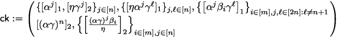
• $\underline{\textsf{Commit}(\textsf{ck}, \boldsymbol{x})}$ returns $\textsf{cm}:=\sum _{j\in [n]} x_j \cdot [ \eta \gamma ^j]_{2} = [\eta p_{\boldsymbol{x}}(\gamma )]_{2}$ and $\textsf{d}:=\boldsymbol{x}$.

• $\underline{\textsf{Open}(\textsf{ck}, \textsf{d}, \textbf{M})}$ Let $\textbf{M} \in \mathbb {Z}_p^{n \times m}$ be an MSP which accepts the input $\boldsymbol{x}$ in $\textsf{d}$. The algorithm computes a witness $\boldsymbol{w} \in \mathbb {Z}_p^{n}$ such that $\textbf{M}^{\top } \cdot ( \boldsymbol{w} \circ \boldsymbol{x}) = \boldsymbol{e}_{1}$, where $\boldsymbol{e}_{1}^{\top } = (1, 0, \ldots , 0)$, and then returns the opening $\textsf{op}:=(\pi _{w}, \pi _{u}, \hat{\pi }) \in \mathbb {G}_1^{3}$ computed as follows:

  $$\begin{aligned} {} & {} \pi _{w} :=\sum _{j \in [n]} w_j \cdot [\alpha ^j]_{1} = [p_{\boldsymbol{w}}(\alpha )]_{1} \\ {} & {} \pi _{u} :=\sum _{j,\ell \in [n]} w_{j} \cdot x_{\ell } \cdot [\eta \alpha ^{j} \gamma ^{\ell }]_{1} = [\eta \cdot p_{\boldsymbol{w}}(\alpha ) \cdot p_{\boldsymbol{x}}(\gamma )]_{1}\\ {} & {} \hat{\pi }:=\sum _{\begin{array}{c} i \in [m] \\ j,k \in [n]: j \ne k \end{array} } \!\! M_{j,i} \cdot x_j \cdot w_k \cdot [\alpha ^{n+1 - j + k} \beta _i \gamma ^{n+1} ]_{1} \, \\ {} & {} \qquad + \sum _{\begin{array}{c} i \in [m] \\ j,k,\ell \in [n]:\ell \ne j \end{array} } M_{j,i} \cdot x_\ell \cdot w_k \cdot \left[ \alpha ^{n+1 - j + k} \beta _i \gamma ^{n+1 - j + \ell } \right] _1 \end{aligned}$$

  Above, $\pi _{w}$ represents a commitment to the witness $\boldsymbol{w} = [p_{\boldsymbol{w}}(\alpha )]_{1}$, $\pi _{u}= [\eta p_{\boldsymbol{w}}(\alpha ) p_{\boldsymbol{x}}(\gamma )]_{1}$ is an encoding of $\boldsymbol{u} = \boldsymbol{w} \circ \boldsymbol{x}$. Finally, $\hat{\pi }$ can be seen as an evaluation proof for the linear map FC of [45] which shows that the vector $\boldsymbol{w}$ committed in $\pi _{w}$ is a solution to the linear system $((\boldsymbol{x} || \cdots || \boldsymbol{x}) \circ \textbf{M})^{\top } \cdot \boldsymbol{w} = \textbf{M}^{\top } \cdot (\boldsymbol{w} \circ \boldsymbol{x}) = \boldsymbol{e}_1$.

• $\underline{\textsf{Verify}(\textsf{ck}, \textsf{cm}, \textsf{op}, \textbf{M}, \textsf{true})}$ Compute $\varPhi \leftarrow \sum _{i \in [m],j \in [m]} M_{j,i} \cdot \left[ \frac{(\alpha \gamma )^{n+1 -j} \beta _i}{\eta } \right] _2$, and output 1 iff the following checks are both satisfied:

  $$\begin{aligned} \hat{e}(\pi _{w}, \textsf{cm}) & {\mathop {=}\limits ^{?}}& \hat{e}( \pi _{u} , [1]_{2} ) \end{aligned}$$

  (3)
  $$\begin{aligned} \hat{e}(\pi _{u}, \varPhi ) & {\mathop {=}\limits ^{?}}& \hat{e}( \hat{\pi }, [1]_{2} ) \cdot \hat{e}( [\alpha \beta _1\gamma ]_{1}, \, [(\alpha \gamma )^{n}]_{2}) \end{aligned}$$

  (4)

Remark 3

In the FC scheme above one can only create an opening if the MSP $\textbf{M}$ accepts the committed input $\boldsymbol{x}$, but not if it rejects. This functionality is enough to build an FC for $\textsf{NC}^{1}$ circuits with a single output. If one wants to open for a circuit C such that $C(\boldsymbol{x})$ outputs 1 then uses the MSP $\textbf{M}_{C}$ associated to C. If on the other hand, one wants to open to C such that $C(\boldsymbol{x})=0$ then one can instead prove that $\bar{C}(\boldsymbol{x})=1$, where $\bar{C}$ is the same as C with a negated output, and then use the MSP $\textbf{M}_{\bar{C}}$ and show that it accepts.

Proof of Security. In the full version [13], we prove the weak evaluation binding of our FC based on the following (falsifiable) assumption. This is a variant of the assumption used in [17], which we justify in the generic group model in the full version[13].

Definition 8

((n, m)-QP-BDHE assumption). Let $\textsf{bp}= (p, \mathbb {G}_1, \mathbb {G}_2, \mathbb {G}_T, \hat{e}, g_1, g_2)$ be a bilinear group setting. The (n, m)-QP-BDHE holds if for every $n,m = \textsf{poly}$ and any PPT $\mathcal {A}$, the following advantage is negligible

$$\textbf{Adv}^{(n,m)\text{- }QP\text{- }BDHE}_{\mathcal {A}}(\lambda ) = \Pr [\mathcal {A}(\textsf{bp}, \varOmega ) = [\alpha ^{n+1} \gamma ^{n+1} \delta ]_T] \quad \mathrm{{ where}}$$

and the probability is over the random choices of , and $\mathcal {A}$’s random coins.

Zero-Knowledge. We discuss how to tweak the FC scheme in such a way that the commitment is hiding and the openings are zero-knowledge.

To do this, we consider an instantiation of the FC for vectors of length $n+1$. Then, a commitment to $\boldsymbol{x}$ is a commitment to $\tilde{\boldsymbol{x}} = (r, \boldsymbol{x})$ where . This way the group element $\textsf{cm}$ is distributed like a uniformly random group element. The second change in the scheme is that in both $\textsf{Open}$ and $\textsf{Verify}$, given an MSP matrix $\textbf{M}$, one runs the same algorithms with a matrix $\tilde{\textbf{M}} = (\boldsymbol{0} \mid \textbf{M}^{\top })^{\top }$, i.e., $\textbf{M}$ with a zero row on top. This way the linear system remains functionally equivalent as r is ignored; this preserves both correctness and binding.

The third change is that $\textsf{Open}$ computes $\pi _{w}$ as a commitment to the vector $\tilde{\boldsymbol{w}} = (s, \boldsymbol{w})$ for a random . This way, $\pi _{w}$ is uniformly distributed. Thanks to the row of zeros in $\tilde{\textbf{M}}$, correctness is preserved.

Finally, to argue that this modified FC satisfies zero-knowledge, we show the simulators (that are assumed to know as trapdoors the values $\alpha , \gamma , \eta , \boldsymbol{\beta }$). $\mathcal {S}_1$ outputs $\textsf{cm}$ as a commitment to $(r, \boldsymbol{0})$ using a random , and stores r in $\textsf {aux}$. $\mathcal {S}_2$ samples , computes $\pi _{u} \leftarrow (\eta \gamma r) \cdot \pi _{w}$ and computes the simulated proof $\hat{\pi }$ as

$$ \hat{\pi }:=\left( \sum _{i \in [m],j \in [m]} M_{j,i} \cdot \frac{(\alpha \gamma )^{n+1 -j} \beta _i}{\eta } \right) \cdot \pi _{u} - [(\alpha \gamma )^{n+1} \beta _1]_{1} $$

which is the unique value satisfying equation (4).

5.2 Other Instantiations

Libert et al.’s FC. The seminal work of Libert et al. [48] constructs FC for linear functions $\mathcal {F}:=\{F: \mathbb {Z}_p^{n} \rightarrow \mathbb {Z}_p\}$, such that each $F$ is defined by a vector $\boldsymbol{\beta }$ and $F_{\boldsymbol{\beta }}(\textbf{x}) = \sum _{i=1}^{n} \textbf{x}_i \boldsymbol{\beta }_i$. Consider a bilinear group setting $\textsf{bp}:=(p, \mathbb {G}_1, \mathbb {G}_2, \mathbb {G}_T, e, g_1, g_2)$. The construction is as follows.

• $\textsf{Setup}(1^\lambda , n)$ samples and returns $\textsf{ck}$ as

  $$ \textsf{ck}:= \left( \{[u^j]_{1}\}_{j \in [2n]\backslash \{n+1\}}, \{[u^j]_{2}\}_{j \in [n]} \right) . $$

  The trapdoor key is defined as $\textsf{td}:= [u^{n+1}]_{1}$.

• $\textsf{Commit}(\textsf{ck}, \textbf{x}; r)$ returns $\textsf{cm}= [r]_{1} + \sum _{j \in [n]} \textbf{x}_j \cdot [u^j]_{1}$ and $\textsf{d}= (\textbf{x}, r)$.

• $\textsf{Open}(\textsf{ck}, \textsf{d}, \boldsymbol{\beta })$ parses $\textsf{d}$ as $\textsf{d}= (\textbf{x}, r)$ and for $y = \langle \textbf{x}, \boldsymbol{\beta }\rangle$, returns ${\textsf{op}_y = \sum _{i \in [n]} \boldsymbol{\beta }_i \cdot W_i}$, where $W_i = r \cdot [u^{n-i+1}]_{1} + \sum _{j \in [n], j \ne i} \textbf{x}_j \cdot [u^{n+1-i+j}]_{1}$.

• $\textsf{Verify}(\textsf{ck}, \textsf{cm}, \textsf{op}_y, \boldsymbol{\beta }, y)$ returns 1 if

  $$ \hat{e}(\textsf{cm}, \sum _{i \in [n]} \boldsymbol{\beta }_i \cdot [u^{n+1-i}]_{2}) {\mathop {=}\limits ^{?}}\hat{e}(\textsf{op}_y, [1]_{2})\cdot \hat{e}([u]_{1}, [u^n]_{2})^y $$

It is clear that the verification is linear in the opening proof. To show the construction provides perfect ZK, an efficient simulator $\mathcal {S}= (\mathcal {S}_1, \mathcal {S}_2)$ can be constructed as follows: $\mathcal {S}_1(\textsf{td})$ first generates $\textsf{cm}:= \textsf{Commit}(\textsf{ck}, \textbf{0}; r)$ and defines $\textsf {aux}:= r$. Now, for any adversarially chosen vector $\textbf{x}$, and any query $\boldsymbol{\beta }$, $\mathcal {S}_2(\textsf{td}, \textsf {aux}, \boldsymbol{\beta }, y = \langle \textbf{x}, \boldsymbol{\beta }\rangle )$ returns $\textsf{op}= r \cdot (\sum _{i \in [n]} \boldsymbol{\beta }_i \cdot [u^{n+1-i}]_{1}) - y \cdot [u^{n+1}]_{1} \in \mathbb {G}_1$.

Lipmaa and Pavlyk’s FC. Limpaa and Pavlyk [50] proposed an FC for a class of circuits $\mathcal {F}:=\{F: \mathcal {D}^{n} \rightarrow \mathcal {D}^{\kappa }\}$ where each $\mathcal {F}$ is defined by a vector $\boldsymbol{\beta }\in \mathcal {D}^{\mu _\beta }$. Their scheme is based on the SNARK construction of Groth16 [37] for $F^*$—a compiled version of $F$. In Groth’s SNARK, the argument consists of three group elements $\pi = ([A]_{1}, [B]_{2}, [C]_{1})$. The key idea in SFC of [50] is as follows: first, express the first two elements $[A]_{1}, [B]_{2}$ as sums of two elements where the first depends only on the secret data and the second depends only on the public data (i.e., $\boldsymbol{\beta }$ and the output $F(\textbf{x}, \boldsymbol{\beta })$). That is, $[A]_{1} = [A_s]_{1} + [A_p]_{1}$ and $[B]_{2} = [B_s]_{2} + [B_p]_{2}$. Next, write $[C]_{1}$ as $[C_{sp}]_{1} + [C_p]_{1}$, where $[C_p]_{1}$ depends only on the public data and $[C_{sp}]_{1}$ depends on both the public and the secret data. Now, a functional commitment to $\textbf{x}$ is $\textsf{cm}= ([A_s]_{1}, [B_s]_{2})$ and the opening to $F(\cdot , \boldsymbol{\beta })$ is $\textsf{op}= [C_{sp}]_{1}$. To verify an opening $\textsf{op}$, the verifier computes $[A_p]_{1}$, $[B_p]_{2}$, and $[C_p]_{1}$, and then runs the SNARK verifier on the argument $([A_s]_{1} + [A_p]_{1}, [B_s]_{2} + [B_p]_{2}, [C_{sp}]_{1} + [C_p]_{1})$. The construction is shown to be perfectly zero-knowledge as defined in [50], but it is not hard to show that it satisfies our stronger definition (i.e., definition 4) as well. In fact, given $\textsf{td}= (u, v)$ as the trapdoor of the commitment key, $\mathcal {S}_1(\textsf{td})$ generates the commitment as the first step of the SNARK simulation in [50] and defines $\textsf {aux}$ as the discrete logarithm of the commitment. Now, $\mathcal {S}_2$ can utilises $\textsf {aux}$ and answer oracle queries for different circuits $F(\cdot , \boldsymbol{\beta })$ by performing the rest of the SNARK simulation. Given that the verification in the SNARK of [37] is linear in the opening $[C_{sp}]_{1}$ makes this functional commitment an appropriate instantiation for our construction of $\textrm{WE}^{\text {FC}}$.

6 From $\textrm{WE}^{\text {FC}}$ to Reusable Non-interactive MPC

6.1 Preliminaries on mrNISC

Here we first recall the definition of mrNISC schemes in [9] and their construction based on $\textrm{WE}^{\text {ZK}\text{- }\text {CM}}$. We then show how our notion of $\textrm{WE}^{\text {FC}}$ can be used as a replacement of $\textrm{WE}^{\text {ZK}\text{- }\text {CM}}$ in their construction.

There are two rounds in mrNISC-style variant of secure multiparty computation protocols, input encoding phase and evaluation phase. In the first round, parties publish encodings of their secret inputs on a public bulletin board, without any coordination with other parties. This happens once and for all. Next, in the second round, any subset of parties can compute a function on their inputs by publishing only one message each. More formally, a mrNISC scheme is defined by the following three algorithms:

• Input Encoding $(\hat{x}_i, s_i) \leftarrow \textsf{Commit}(1^\lambda , x_i)$ by which a party $P_i$ encodes its private input $x_i$ and publishes the encoding $\hat{x}_i$.

• Computation Encoding $\eta _i \leftarrow \textsf{Encode}(z, \{\hat{x}_j\}_{j \in J}, s_i)$ by which each party $P_i$ among a subset of parties $\{ P_j \}_{j \in J}$ generates and publishes a computation encoding $\eta _i$. This allows parties in J to compute a functionality f described by z (i.e., $f(z, \star )$) on their private inputs.

• Output $y = \textsf{Eval}(z, \{\hat{x}_j\}_{j \in J}, \{ \eta _j\}_{j \in J})$ which deterministically computes the output y (required to be $f(z, \{x_j\}_{j \in J})$ by the correctness property).

The construction of mrNISC in [9] is based upon the work of [34], where they follow the round collapsing approach for constructing 2-round MPC protocols used in [27]. Let $\prod$ be an L-round MPC protocol. The round collapsing approach collapses $\prod$ into a 2-round protocol $\overline{\prod }$ as follows. For $\ell \in [L]$, let $m_i^{\ell }$ denote the message published by party $P_i$ in round $\ell$ of $\prod$. Let $x_i$ and $r_i$ be respectively the secret input and random tape of $P_i$ used to execute $\prod$. In the first round of $\overline{\prod }$, each party $P_i$ commits to its private input $(x_i, r_i)$ and broadcasts the resulting commitment $\textsf{cm}_i$. In the second round, each party $P_i$ garbles its next-step message function $F_i^{\ell }$ in $\prod$ for each round $\ell \in [L]$. Note that the resulting garbled circuit, denoted by $\hat{F}_i^{\ell }$, should take as input all the messages $\textbf{m}^{<\ell } = \{m_j^\ell \}_{l<\ell , j \in [n]}$ of all parties up to round $\ell -1$, and outputs the next message $m_i^\ell$ of $P_i$ in $\prod$. To do so, each $P_i$ should provide a way for other parties to compute the labels of $\hat{F}_i^\ell$ that correspond to the correct messages in $\prod$, where a message $m_j^{l}$ is correct if it is computed from $P_i$’s committed messages $(x_i, r_i)$ in the first round. To this end, [34] suggests the following mechanism: let $k_0$ and $k_1$ be two labels for an input wire in $P_i$’s garbled circuit $\hat{F}_i^\ell$. Suppose that $\hat{F}_i^\ell$ takes as input the t’th bit $y = m_{j,t}^{l}$ of a message from $P_j$ (where $m_j^{l}$ is output by $P_j$’s garbled circuit $\hat{F}_j^{l}$), and provides a way for all parties to obtain the valid label $k_y$. The key idea in [34] is to use a general-purpose WE to produce a ciphertext $\textsf{ct}_y \leftarrow \textsf{WE}.\textsf{Enc}(\textsf{x}_y, k_y)$ for $y \in \{0, 1\}$ under the statement $\textsf{x}_y$ that “there exists a NIZK proof $\pi _y$ that proves $y = m_{j,t}^{l}$ is computed correctly”. Again, correct computation here means that y is computed from $P_j$’s committed messages $(x_i, r_i)$ in the first round, and in accordance to the partial transcript of messages $\textbf{m}^{<l}$. The two ciphertexts $(\textsf{ct}_0, \textsf{ct}_1)$ are part of what $P_i$ in the garbled circuit $\hat{F}_i^{l}$ outputs. Furthermore, to allow all parties to (publicly) obtain the correct label $k_y$, $P_j$’s garbled circuit $\hat{F}_j^l$ additionally outputs a NIZK proof $\pi _y$ that $y = m_{j,t}^{l}$ is correctly computed. Correctness of $\overline{\prod }$ follows from correctness of WE. Security also follows from the fact that $k_{1-y}$ remains hidden by the soundness of NIZK and semantic security of WE. Furthermore, the ZK property of NIZK guarantees the privacy of parties.

The main problem in the above construction of [34] is the lack of general-purpose WE from standard assumptions. Benhamouda and Lin [9] overcome this problem by observing that not a WE for general NP language, but a WE scheme for a particular language corresponding to the verification circuit of a NIZK proof that proves the correctness of computation over committed information suffices to realize the above construction. This variant of WE, denoted by $\textrm{WE}^{\text {ZK}\text{- }\text {CM}}$ in this work, consists of a triple $\textsf{WE}^{\textsf{ZK}\text{- }\textsf{CM}}= (\textsf{COM}, \textsf{NIZK}, \textsf{WE})$ and is defined for a NP language $\mathcal {L}$ such that a statement $\textsf{x}= (\textsf{cm}, G, y)$ is in $\mathcal {L}$ iff there exists an accepting NIZK proof $\pi$ (as the witness for $\textsf{x}$) w.r.t. $\textsf{crs}$ that proves $\textsf{cm}$ is a commitment of some value v and that $G(v)=y$. As provided in the construction of [34] (but based on stronger assumption of general-purpose WE), $\textrm{WE}^{\text {ZK}\text{- }\text {CM}}$ should support all polynomial computations; i.e., it should be that G in the statements $\textsf{x}= (\textsf{cm}, G, y)$ can be any arbitrary polynomial-sized circuit. Moreover, the commitments in $\textrm{WE}^{\text {ZK}\text{- }\text {CM}}$ should be reusable in the sense that generating unbounded number of NIZK proofs and WE ciphertexts w.r.t. commitments should not reveal any information about the committed (secret) values, except what is revealed by the statements. Equipped with this property then allows to make the construction of [34] reusable by replacing $r_i$ with a PRF seed $s_i$ that generates pseudo-random tapes for an unbounded number of computations. The key idea in the construction of $\textrm{WE}^{\text {ZK}\text{- }\text {CM}}$ in [9] is to use a NIZK proof system that has a linear-decision verification. Given such NIZK is then sufficient to realize $\textrm{WE}^{\text {ZK}\text{- }\text {CM}}$ using a WE for linear languages which can be constructed efficiently based on SPHFs. In more details, let $\mathbf {\Theta }= \textbf{M}\pi$ be the linear equation corresponding to the verification of NIZK for a statement $\textsf{x}= (\textsf{cm}, G, y)$, such that $\mathbf {\Theta }$ and $\textbf{M}$ depend on $\textsf{x}$ and thus are known at the time of encryption. One can now encrypt a message straightforwardly by using an SPHF for this relation such that only one who can compute the hash value using a valid witness $\pi$ can retrieve the message.

6.2 Our mrNISC Construction

We now show how one can replace $\textrm{WE}^{\text {ZK}\text{- }\text {CM}}$ with $\textrm{WE}^{\text {FC}}$ in the aforementioned construction. Let $\textsf{FC}$ be a succinct functional commitment for circuit class $\mathcal {F}$, and $\textsf{WE}^{\textsf{FC}}= (\textsf{Setup}, \textsf{Commit}, \textsf{Open}, \textsf{Verify}, \textsf{Enc}, \textsf{Dec})$ be a $\textrm{WE}^{\text {FC}}$ for $\mathcal {F}$ constructed as in Sect. 4.2. Besides $\textsf{WE}^{\textsf{FC}}$, the construction uses the following building blocks, formally defined in the full version [13]:

• A semi-malicious output-delayed simulatable L-round MPC protocol $\prod = (\textsf{Next}, \textsf{Output})$ for f.

• A garbled circuit $\textsf{GC}= (\textsf{Gen}, \textsf{Garble}, \textsf{Eval}, \textsf{Sim})$ for $\mathcal {F}$.

The construction is as follows:

• Input Encoding. For a binary input $x_i$ and PRF key , party $P_i$ commits to $x_i||fk_i$ as $(\textsf{cm}_i, \textsf{d}_i) \leftarrow \textsf{Commit}(\textsf{ck}, (x_i||fk_i); r_i)$. It then sets $\hat{x}_i:= \textsf{cm}_i$ and $s_i := (x_i, fk_i, \textsf{d}_i)$.

• Computation Encoding. To encode a computation $f(z, \star )$, each party $P_i$ for $\ell \in [L]$ generates input labels $(\textbf{st}\textbf{E}^{\ell }_{i}, \{\textbf{msg}\textbf{E}^{\ell }_{i,j}\}_{j \in J}) \leftarrow \textsf{Gen}(1^\lambda )$ and garbles the evaluation function $\textbf{F}^{\ell }_{i}$ (defined in Fig. 3) as $\hat{\textbf{F}}^{\ell }_{i} \leftarrow \textsf{Garble}((\textbf{st}\textbf{E}^{\ell }_{i}, \{\textbf{msg}\textbf{E}^{\ell }_{i,j}\}_{j \in J}), \textbf{F}^{\ell }_{i})$. Finally, it sets $\eta _i := \{\hat{\textbf{F}}^{\ell }_{i}\}_{\ell \in [L]}$.

• Output. The output is computed by recovering the input labels and then evaluating the garbled circuits on them in L iteration. That is, for $\ell = 1, \ldots , L$:

  • 1. For $i \in J$,

    $$ \left( \textbf{st}\textbf{E}'^{\ell +1}_{i}, \{\textsf{ct}^{\ell }_{i, j, k, b}\}_{j, k, b}, m^{\ell }_i, \{\textsf{op}^{\ell }_{i, k}\}_{k}\right) := \textsf{Eval}(\hat{\textbf{F}}^{}_{i}, (\textbf{st}\textbf{E}'^{\ell }_{i}, \{\textbf{msg}\textbf{E}^{\ell }_{i,j}[m^{\ell -1}_{j}]\}_{j \in J})). $$

  • 2. If $\ell \ne L$, then for $i,j \in J$ and $k \in [\nu _m]$,

    $$ \textbf{msg}\textbf{E}^{\ell +1}_{i,j}[m^{\ell }_j] := \Big \{ \textsf{Dec}(\textsf{ck}, \textsf{ct}^{\ell +1}_{i, j, k, m^{\ell }_{j,k}}, \textsf{cm}_j, G^{\ell }_{j,k}, m^{\ell }_{j,k}, \textsf{op}^{\ell }_{i,j,k}) \Big \} $$

  After all the messages $\textbf{m}= \{m^{\ell }_{j}\}_{j \in J, \ell \in [L]}$ of the inner MPC are recovered, the final output is computed as $y := \textsf{Output}(z, \textbf{m})$.

The correctness of the construction follows straightforwardly from the correctness of the underlying building blocks. For security, we refer to [9] as the proof is similar to the security of the mrNISC construction in [9]. Here, we only state the theorem.

Fig. 3.

Circuit $\textbf{F}^{\ell }_{i}$ for the construction of mrNISC based on $\textrm{WE}^{\text {FC}}$

Theorem 4

Let $\textsf{PRF}$ be a pseudorandom function, $\textsf{GC}$ be a garbled circuit with simulatability property, $\prod$ be a semi-malicious output-delayed simulatable MPC protocol, and $\textsf{WE}^{\textsf{FC}}$ be a $\textrm{WE}^{\text {FC}}$ with semantic security. The mrNISC scheme described above is semi-maliciously private.

On the Efficiency of our mrNISC Construction. The main advantage of our mrNISC construction compared to the one in [9] is that our approach admits an input encoding phase with much shorter communication since we use succinct commitments. This is especially important since commitments are supposed to be stored in a public bulletin board to be re-used in several future computations.

Remark 4

While our FC construction can be used to instantiate our $\textrm{WE}^{\text {FC}}$ for $\textsf{NC}^{1}$, we need one to support arbitrary circuits to instantiate our mrNISC (roughly, this corresponds to the round function of the “lifted” MPC, plus PRFs). To achieve this, we notice we can use the same generic bootstrapping technique used in [9] to obtain $\textrm{WE}^{\text {FC}}$ for all polynomial-size circuits. For a polynomial-size computation $G(v)=y$, the bootstrapping technique encodes the computation into a randomized encoding $o = \textsf{RE}(G, v, \textsf{PRF}(k))$ (for some PRF seed k) that reveals y. Given that both $\textsf{RE}$ and $\textsf{PRF}$ are computable in $\textsf{NC}^{1}$, our $\textrm{WE}^{\text {FC}}$ for $\textsf{NC}^{1}$ can be used to verify if the computation of o from (v, k)—committed in a commitment $\textsf{cm}$—is correct. There is still one issue left that verifying that o decodes to y is still in $\textsf {P}$. To get around this, a garbled circuit is instead used to verify if a given input $o'$ decodes to y.

We observe that this technique preserves the succinctness of the encoding (commitments) in the context of mrNISC protocols.

7 Other Application Scenarios

In this section we show that our notion of $\textrm{WE}^{\text {FC}}$can be versatile; we describe how it can be used in other scenarios besides mrNISC.

7.1 Targeted Broadcast

As a first application scenario, we discuss how to apply $\textrm{WE}^{\text {FC}}$ to a targeted broadcast with “special properties”. See last item in Sect. 1.2 for a description of the problem, but a quick summary is: we aim at encrypting a message with respect to some attributes (not necessarily known before encryption time); only users holding those attributes can decrypt (we discuss later how they are granted).

This subsection proceeds in three parts. We first give a flavor of our approach template, which we call “commit-and-receive” since it involves a commitment to user attributes which allows them to decrypt to compatible messages. We then argue what properties make this approach interesting compared to the more standard targeted broadcast setting. Finally we compare to alternative approaches in more detail. Due to the lack of space, the last two parts are deferred to the full version [13].

Our Approach: Commit-and-Receive. We now describe our general approach. To better provide an intuition for it, we start with a flavor of which settings it is suitable for; this is best introduced through a specific toy example. Consider a sophisticated programming contest where participants are asked to write a program solving a specific algorithmic problem. To evaluate each submission, it is common for the organizers to execute the program against several test cases (not public before submission deadline). If submission passes enough test-cases, the sender can receive instructions to move on to the next stage (or receive a digital prize, e.g. a full copy of TAOCP¹⁶). If the participants want to keep their code secret, can their program still be tested and receive the instructions/prize? There are arguably other natural settings besides this one¹⁷.

We aim at providing a solution for a generalized version of the setting above with particular attention at minimizing round interaction. We call our approach “Commit-and-Receive”¹⁸ and we show how it can be naturally built through our primitive $\textrm{WE}^{\text {FC}}$.

Our approach, described through the lens of the application example above: consider a party R interested in receiving some message (e.g. a digital good) from a sender S. The latter would like the message to be received by R only if some data $D_R$ held by R satisfy a certain policy (e.g. the tests determined which programs will pass the contest or the drawn lottery number). The data $D_R$ are committed beforehand and the policy is not chosen adaptively and thus possibly not known at commitment time. After each participant has published a commitment $\textsf{cm}_i$ to their program, the organizers can broadcast $\boldsymbol{\mathsf {\textsf{ct}}} := \left( \textsf{ct}_1, \dots , \textsf{ct}_\ell \right)$ with $\textsf{ct}_i \leftarrow \textsf{WE}^{\textsf{FC}}.\textsf{Enc}(\textsf{ck}, \textsf{cm}_i, F_\mathrm{{tests}}, m)$, where m contains further instructions or a digital prize and $F_\mathrm{{tests}}$ is a function checking if tests are passed. The participants whose solutions do not pass the tests will not be able to decrypt their respective ciphertext.

7.2 Simple Contingent Payment for Services

The next application setting we describe has to do with a form of conditional payments. Imagine we want to incentivize the availability of some large data (Internet Archive, Wikipedia, etc.). One approach to (publicly) check data availability uses some variant of this approach: for the data D there exists a public, succinct commitment (e.g., a Merkle Tree or a functional commitment compatible with $\textrm{WE}^{\text {FC}}$ in our case); once every epoch, a verifier samples random indices ; a storage provider shows an opening (e.g., Merkle tree paths) to the values $D[r_1], \dots , D[r_m]$. If carried out enough times and appropriately choosing m, this procedure can guarantee data availability with low communication [41]. Notice that the use of succinct commitments is essential in such an application: if verification requires the same amount of storage as the data D, one may be better off storing D.

There are several approaches to incentivizing availability without the need of interaction from the party interested in keeping the data available (which we call stakeholder in the remainder). Several of these approaches involve embedding incentives in the mining process in a blockchain (e.g., Filecoin) or letting a smart contract (e.g., on Ethereum) unlock a reward¹⁹ if the verification process above succeeds. Other solutions apply threshold cryptography requiring a set of parties to be available and act as decryptor oracles [44]. Through $\textrm{WE}^{\text {FC}}$, we can achieve a simpler solution that does not rely on threshold networks, a specific blockchain architecture or smart contracts (convenient both in terms of gas costs, simplicity and communication complexity on chain) . The solution is as follows. The stakeholder produces a vector of random indices $\boldsymbol{r}$ as above and produces the ciphertext $\textsf{ct} \leftarrow \textsf{WE}^{\textsf{FC}}.\textsf{Enc}(\textsf{ck}, \textsf{cm}_D, F_{\boldsymbol{r}}, \textsf{k}_\mathrm{{ca}\$\textrm{h}})$ where $\textsf{cm}_D$ is a commitment to the data, $F_{\boldsymbol{r}}$ is a selector function—$F_{\boldsymbol{r}}(D) := \left( D[r_1], \dots , D[r_m] \right)$—and $\textsf{k}_\mathrm{{ca}\$\textrm{h}}$ is the message we are encrypting, that is a secret that allows access to the reward (e.g., a Bitcoin private key). Further subtleties of this approach are discussed in the full version [13]. We believe the solution above can be applied generically to other natural settings.

An important note is that for the approach above to work we need a stronger variant of $\textrm{WE}^{\text {FC}}$ in which (a) the encryptor does not need to know the output of the function used in the statement, and (2) security has an extractability flavor which ensures that a successful decryptor will actually know the output of $F_{\boldsymbol{r}}(D)$ for committed data D. In the full version [13], we define this variant of $\textrm{WE}^{\text {FC}}$ and prove that our same construction of Sect. 4 satisfies this stronger property.

References

Decentralized storage. https://ethereum.org/en/developers/docs/storage/ (2022)
Abdalla, M., Benhamouda, F., MacKenzie, P.: Security of the J-PAKE password-authenticated key exchange protocol. In: 2015 IEEE Symposium on Security and Privacy, pp. 571–587. IEEE Computer Society Press (2015). https://doi.org/10.1109/SP.2015.41
Abdalla, M., Benhamouda, F., Pointcheval, D.: Disjunctions for hash proof systems: new constructions and applications. In: Oswald, E., Fischlin, M. (eds.) EUROCRYPT 2015. LNCS, vol. 9057, pp. 69–100. Springer, Heidelberg (2015). https://doi.org/10.1007/978-3-662-46803-6_3
Albrecht, M.R., Cini, V., Lai, R.W.F., Malavolta, G., Thyagarajan, S.A.K.: Lattice-based SNARKs: publicly verifiable, preprocessing, and recursively composable: (extended abstract). In: Dodis, Y., Shrimpton, T. (eds.) Advances in Cryptology – CRYPTO 2022: 42nd Annual International Cryptology Conference, CRYPTO 2022, Santa Barbara, CA, USA, August 15–18, 2022, Proceedings, Part II, pp. 102–132. Springer, Cham (2022). https://doi.org/10.1007/978-3-031-15979-4_4
Balbás, D., Catalano, D., Fiore, D., Lai, R.W.F.: Chainable functional commitments for unbounded-depth circuits. In: Rothblum, G., Wee, H. (eds.) Theory of Cryptography: 21st International Conference, TCC 2023, Taipei, Taiwan, November 29–December 2, 2023, Proceedings, Part III, pp. 363–393. Springer, Cham (2023). https://doi.org/10.1007/978-3-031-48621-0_13
Barta, O., Ishai, Y., Ostrovsky, R., Wu, D.J.: On succinct arguments and witness encryption from groups. In: Micciancio, D., Ristenpart, T. (eds.) Advances in Cryptology – CRYPTO 2020: 40th Annual International Cryptology Conference, CRYPTO 2020, Santa Barbara, CA, USA, August 17–21, 2020, Proceedings, Part I, pp. 776–806. Springer, Cham (2020). https://doi.org/10.1007/978-3-030-56784-2_26
Benhamouda, F., Blazy, O., Chevalier, C., Pointcheval, D., Vergnaud, D.: New techniques for SPHFs and efficient one-round PAKE protocols. In: Canetti, R., Garay, J.A. (eds.) Advances in Cryptology – CRYPTO 2013, pp. 449–475. Springer, Berlin, Heidelberg (2013). https://doi.org/10.1007/978-3-642-40041-4_25
Benhamouda, F., Jain, A., Komargodski, I., Lin, H.: Multiparty reusable non-interactive secure computation from LWE. In: Canteaut, A., Standaert, F.-X. (eds.) Advances in Cryptology – EUROCRYPT 2021: 40th Annual International Conference on the Theory and Applications of Cryptographic Techniques, Zagreb, Croatia, October 17–21, 2021, Proceedings, Part II, pp. 724–753. Springer, Cham (2021). https://doi.org/10.1007/978-3-030-77886-6_25
Benhamouda, F., Lin, H.: Mr NISC: multiparty reusable non-interactive secure computation. In: Pass, R., Pietrzak, K. (eds.) Theory of Cryptography: 18th International Conference, TCC 2020, Durham, NC, USA, November 16–19, 2020, Proceedings, Part II, pp. 349–378. Springer, Cham (2020). https://doi.org/10.1007/978-3-030-64378-2_13
Bernhard, D., Fischlin, M., Warinschi, B.: On the hardness of proving CCA-security of signed ElGamal. In: Cheng, C.-M., Chung, K.-M., Persiano, G., Yang, B.-Y. (eds.) Public-Key Cryptography – PKC 2016: 19th IACR International Conference on Practice and Theory in Public-Key Cryptography, Taipei, Taiwan, March 6-9, 2016, Proceedings, Part I, pp. 47–69. Springer, Berlin, Heidelberg (2016). https://doi.org/10.1007/978-3-662-49384-7_3
Boneh, D., Franklin, M.K.: Identity based encryption from the Weil pairing. SIAM J. Comput. 32(3), 586–615 (2003)
Campanelli, M., David, B., Khoshakhlagh, H., Kristensen, A.K., Nielsen, J.B.: Encryption to the future: a paradigm for sending secret messages to future (anonymous) committees. In: IACR Cryptology ePrint Archive, p. 1423 (2021). https://eprint.iacr.org/2021/1423
Campanelli, M., Fiore, D., Khoshakhlagh, H.: Witness encryption for succinct functional commitments and applications. IACR Cryptol. ePrint Arch., p. 1510 (2022). https://eprint.iacr.org/2022/1510
Campanelli, M., Fiore, D., Querol, A.: LegoSNARK: modular design and composition of succinct zero-knowledge proofs. In: Cavallaro, L., Kinder, J., Wang, X., Katz, J. (eds.) ACM CCS 2019, pp. 2075–2092. ACM Press (2019). https://doi.org/10.1145/3319535.3339820
Campanelli, M., Gennaro, R., Goldfeder, S., Nizzardo, L.: Zero-knowledge contingent payments revisited: attacks and payments for services. In: Thuraisingham, B.M., Evans, D., Malkin, T., Xu, D. (eds.) ACM CCS 2017, pp. 229–243. ACM Press (2017). https://doi.org/10.1145/3133956.3134060
de Castro, L., Peikert, C.: Functional commitments for all functions, with transparent setup and from SIS. In: Hazay, C., Stam, M. (eds.) Advances in Cryptology – EUROCRYPT 2023: 42nd Annual International Conference on the Theory and Applications of Cryptographic Techniques, Lyon, France, April 23-27, 2023, Proceedings, Part III, pp. 287–320. Springer, Cham (2023). https://doi.org/10.1007/978-3-031-30620-4_10
Catalano, D., Fiore, D., Tucker, I.: Additive-homomorphic functional commitments and applications to homomorphic signatures. In: Agrawal, S., Lin, D. (eds.) Advances in Cryptology – ASIACRYPT 2022: 28th International Conference on the Theory and Application of Cryptology and Information Security, Taipei, Taiwan, December 5–9, 2022, Proceedings, Part IV, pp. 159–188. Springer, Cham (2022). https://doi.org/10.1007/978-3-031-22972-5_6
Chen, J., Gay, R., Wee, H.: Improved dual system ABE in prime-order groups via predicate encodings. In: Oswald, E., Fischlin, M. (eds.) Advances in Cryptology - EUROCRYPT 2015: 34th Annual International Conference on the Theory and Applications of Cryptographic Techniques, Sofia, Bulgaria, April 26-30, 2015, Proceedings, Part II, pp. 595–624. Springer, Berlin, Heidelberg (2015). https://doi.org/10.1007/978-3-662-46803-6_20
Chen, J., Gong, J., Kowalczyk, L., Wee, H.: Unbounded ABE via bilinear entropy expansion, revisited. In: Nielsen, J.B., Rijmen, V. (eds.) Advances in Cryptology – EUROCRYPT 2018: 37th Annual International Conference on the Theory and Applications of Cryptographic Techniques, Tel Aviv, Israel, April 29 - May 3, 2018 Proceedings, Part I, pp. 503–534. Springer, Cham (2018). https://doi.org/10.1007/978-3-319-78381-9_19
Chen, Y., Vaikuntanathan, V., Wee, H.: GGH15 beyond permutation branching programs: proofs, attacks, and candidates. In: Shacham, H., Boldyreva, A. (eds.) Advances in Cryptology – CRYPTO 2018: 38th Annual International Cryptology Conference, Santa Barbara, CA, USA, August 19–23, 2018, Proceedings, Part II, pp. 577–607. Springer, Cham (2018). https://doi.org/10.1007/978-3-319-96881-0_20
Couteau, G., Hartmann, D.: Shorter non-interactive zero-knowledge arguments and ZAPs for algebraic languages. In: Micciancio, D., Ristenpart, T. (eds.) Advances in Cryptology – CRYPTO 2020: 40th Annual International Cryptology Conference, CRYPTO 2020, Santa Barbara, CA, USA, August 17–21, 2020, Proceedings, Part III, pp. 768–798. Springer, Cham (2020). https://doi.org/10.1007/978-3-030-56877-1_27
Cramer, R., Shoup, V.: Universal hash proofs and a paradigm for adaptive chosen ciphertext secure public-key encryption. In: Knudsen, L.R. (ed.) Advances in Cryptology—EUROCRYPT 2002, pp. 45–64. Springer, Berlin, Heidelberg (2002). https://doi.org/10.1007/3-540-46035-7_4
Daian, P., Pass, R., Shi, E.: Snow White: robustly reconfigurable consensus and applications to provably secure proof of stake. In: Goldberg, I., Moore, T. (eds.) Financial Cryptography and Data Security: 23rd International Conference, FC 2019, Frigate Bay, St. Kitts and Nevis, February 18–22, 2019, Revised Selected Papers, pp. 23–41. Springer, Cham (2019). https://doi.org/10.1007/978-3-030-32101-7_2
Diffie, W., Hellman, M.E.: New directions in cryptography. IEEE Trans. Inf. Theory 22(6), 644–654 (1976). https://doi.org/10.1109/TIT.1976.1055638
Fernando, R., Jain, A., Komargodski, I.: Maliciously-secure MrNISC in the plain model. In: IACR Cryptology ePrint Archive, p. 1319 (2021). https://eprint.iacr.org/2021/1319
Fuchsbauer, G., Kiltz, E., Loss, J.: The algebraic group model and its applications. In: Shacham, H., Boldyreva, A. (eds.) Advances in Cryptology – CRYPTO 2018: 38th Annual International Cryptology Conference, Santa Barbara, CA, USA, August 19–23, 2018, Proceedings, Part II, pp. 33–62. Springer, Cham (2018). https://doi.org/10.1007/978-3-319-96881-0_2
Garg, S., Gentry, C., Halevi, S., Raykova, M.: Two-round secure MPC from indistinguishability obfuscation. In: Lindell, Y. (ed.) Theory of Cryptography, pp. 74–94. Springer, Berlin, Heidelberg (2014). https://doi.org/10.1007/978-3-642-54242-8_4
Garg, S., Gentry, C., Halevi, S., Raykova, M., Sahai, A., Waters, B.: Candidate indistinguishability obfuscation and functional encryption for all circuits. In: 54th FOCS, IEEE Computer Society Press, pp. 40–49 (2013). https://doi.org/10.1109/FOCS.2013.13
Garg, S., Gentry, C., Sahai, A., Waters, B.: Witness encryption and its applications. In: Boneh, D., Roughgarden, T., Feigenbaum, J. (eds.) In: 45th ACM STOC, pp. 467–476. ACM Press (2013). https://doi.org/10.1145/2488608.2488667
Gennaro, R., Lindell, Y.: A framework for password-based authenticated key exchange. ACM Trans. Inf. Syst. Secur. 9(2), 181–234 (2006)
Gentry, C., Lewko, A., Waters, B.: Witness encryption from instance independent assumptions. In: Garay, J.A., Gennaro, R. (eds.) CRYPTO 2014. LNCS, vol. 8616, pp. 426–443. Springer, Heidelberg (2014). https://doi.org/10.1007/978-3-662-44371-2_24
Gentry, C., Wichs, D.: Separating succinct non-interactive arguments from all falsifiable assumptions. In: Fortnow, L., Vadhan, S.P. (eds.) 43rd ACM STOC, pp. 99–108. ACM Press (2011). https://doi.org/10.1145/1993636.1993651
Goldreich, O., Levin, L.A.: A hard-core predicate for all one-way functions. In: 21st ACM STOC, pp. 25–32. ACM Press (1989). https://doi.org/10.1145/73007.73010
Dov Gordon, S., Liu, F.-H., Shi, E.: Constant-round MPC with fairness and guarantee of output delivery. In: Gennaro, R., Robshaw, M. (eds.) CRYPTO 2015. LNCS, vol. 9216, pp. 63–82. Springer, Heidelberg (2015). https://doi.org/10.1007/978-3-662-48000-7_4
Goyal, R., Koppula, V., Waters, B.: Lockable obfuscation. In: Umans, C. (ed.) 58th FOCS, pp. 612–621. IEEE Computer Society Press (2017). https://doi.org/10.1109/FOCS.2017.62
Goyal, V., Pandey, O., Sahai, A., Waters, B.: Attribute-based encryption for fine-grained access control of encrypted data. In: Juels, A., Wright, R.N., De Capitani di Vimercati, S. (eds.) ACM CCS 2006, pp. 89–98. ACM Press (2006). https://doi.org/10.1145/1180405.1180418, available as Cryptology ePrint Archive Report 2006/309
Groth, J.: On the size of pairing-based non-interactive arguments. In: Fischlin, M., Coron, J.-S. (eds.) EUROCRYPT 2016. LNCS, vol. 9666, pp. 305–326. Springer, Heidelberg (2016). https://doi.org/10.1007/978-3-662-49896-5_11
Groth, J., Sahai, A.: Efficient non-interactive proof systems for bilinear groups. In: Smart, N. (ed.) EUROCRYPT 2008. LNCS, vol. 4965, pp. 415–432. Springer, Heidelberg (2008). https://doi.org/10.1007/978-3-540-78967-3_24
Hamouda-Guichoux, F.B.: Diverse modules and zero-knowledge. Ph.D. thesis, École Normale Supérieure, Paris, France (2016). https://tel.archives-ouvertes.fr/tel-01399476
Jain, A., Lin, H., Sahai, A.: Indistinguishability obfuscation from well-founded assumptions. In: Proceedings of the 53rd Annual ACM SIGACT Symposium on Theory of Computing, pp. 60–73 (2021)
Juels, A., Kaliski Jr., B.S.: PORs: proofs of retrievability for large files. In: Ning, P., De Capitani di Vimercati, S., Syverson, P.F. (eds.) ACM CCS 2007, pp. 584–597. ACM Press (2007). https://doi.org/10.1145/1315245.1315317
Karchmer, M., Wigderson, A.: On span programs. In: [1993] Proceedings of the Eighth Annual Structure in Complexity Theory Conference, pp. 102–111 (1993)
Khoshakhlagh, H.: (Commit-and-prove) predictable arguments with privacy. In: Ateniese, G., Venturi, D. (eds.) ACNS 22. LNCS, vol. 13269, pp. 542–561. Springer, Heidelberg (2022). https://doi.org/10.1007/978-3-031-09234-3_27
Kokoris-Kogias, E., et al.: CALYPSO: auditable sharing of private data over blockchains. Cryptology ePrint Archive, Report 2018/209 (2018). https://eprint.iacr.org/2018/209
Lai, R.W.F., Malavolta, G.: Subvector commitments with application to succinct arguments. In: Boldyreva, A., Micciancio, D. (eds.) CRYPTO 2019. LNCS, vol. 11692, pp. 530–560. Springer, Cham (2019). https://doi.org/10.1007/978-3-030-26948-7_19
Lewko, A., Okamoto, T., Sahai, A., Takashima, K., Waters, B.: Fully secure functional encryption: attribute-based encryption and (hierarchical) inner product encryption. In: Gilbert, H. (ed.) EUROCRYPT 2010. LNCS, vol. 6110, pp. 62–91. Springer, Heidelberg (2010). https://doi.org/10.1007/978-3-642-13190-5_4
Lewko, A., Waters, B.: Unbounded HIBE and attribute-based encryption. In: Paterson, K.G. (ed.) EUROCRYPT 2011. LNCS, vol. 6632, pp. 547–567. Springer, Heidelberg (2011). https://doi.org/10.1007/978-3-642-20465-4_30
Libert, B., Ramanna, S.C., Yung, M.: Functional commitment schemes: from polynomial commitments to pairing-based accumulators from simple assumptions. In: Chatzigiannakis, I., Mitzenmacher, M., Rabani, Y., Sangiorgi, D. (eds.) ICALP 2016. LIPIcs, vol. 55, pp. 30:1–30:14. Schloss Dagstuhl (2016). https://doi.org/10.4230/LIPIcs.ICALP.2016.30
Lipmaa, H.: Prover-efficient commit-and-prove zero-knowledge SNARKs. In: Pointcheval, D., Nitaj, A., Rachidi, T. (eds.) AFRICACRYPT 2016. LNCS, vol. 9646, pp. 185–206. Springer, Cham (2016). https://doi.org/10.1007/978-3-319-31517-1_10
Lipmaa, H., Pavlyk, K.: Succinct functional commitment for a large class of arithmetic circuits. In: Moriai, S., Wang, H. (eds.) ASIACRYPT 2020. LNCS, vol. 12493, pp. 686–716. Springer, Cham (2020). https://doi.org/10.1007/978-3-030-64840-4_23
Sahai, A., Waters, B.: Fuzzy identity-based encryption. In: Cramer, R. (ed.) EUROCRYPT 2005. LNCS, vol. 3494, pp. 457–473. Springer, Heidelberg (2005). https://doi.org/10.1007/11426639_27
Shamir, A.: Identity-based cryptosystems and signature schemes. In: Blakley, G.R., Chaum, D. (eds.) CRYPTO 1984. LNCS, vol. 196, pp. 47–53. Springer, Heidelberg (1985). https://doi.org/10.1007/3-540-39568-7_5
Wee, H.: Efficient chosen-ciphertext security via extractable hash proofs. In: Rabin, T. (ed.) CRYPTO 2010. LNCS, vol. 6223, pp. 314–332. Springer, Heidelberg (2010). https://doi.org/10.1007/978-3-642-14623-7_17
Wee, H., Wu, D.J.: Succinct vector, polynomial, and functional commitments from lattices. In: Hazay, C., Stam, M. (eds.) EUROCRYPT 2023, Part III. LNCS, vol. 14006, pp. 385–416. Springer, Heidelberg (2023). https://doi.org/10.1007/978-3-031-30620-4_13
Wichs, D., Zirdelis, G.: Obfuscating compute-and-compare programs under LWE. In: Umans, C. (ed.) 58th FOCS, pp. 600–611. IEEE Computer Society Press (2017). https://doi.org/10.1109/FOCS.2017.61
Acknowledgements
This work has received funding from the European Research Council (ERC) under the European Union’s Horizon 2020 research and innovation programme under project PICOCRYPT (grant agreement No. 101001283), and from the Spanish Government MCIN/AEI/10.13039/501100011033/ under projects PRODIGY (TED2021-132464B-I00) and ESPADA (PID2022-142290OB-I00). The last two projects are co-funded by European Union FEDER and NextGenerationEU/PRTR funds.
Author information
Authors and Affiliations
Corresponding author
Editor information
Editors and Affiliations
Rights and permissions
Copyright information
© 2024 International Association for Cryptologic Research
About this paper
Cite this paper
Campanelli, M., Fiore, D., Khoshakhlagh, H. (2024). Witness Encryption for Succinct Functional Commitments and Applications. In: Tang, Q., Teague, V. (eds) Public-Key Cryptography – PKC 2024. PKC 2024. Lecture Notes in Computer Science, vol 14602. Springer, Cham. https://doi.org/10.1007/978-3-031-57722-2_5
Download citation
DOI: https://doi.org/10.1007/978-3-031-57722-2_5
Published:
Publisher Name: Springer, Cham
Print ISBN: 978-3-031-57721-5
Online ISBN: 978-3-031-57722-2
eBook Packages: Computer ScienceComputer Science (R0)