
Abstract
We introduce a toolkit for transforming lattice-based hash-and-sign signature schemes into masking-friendly signatures secure in the t-probing model. Until now, efficiently masking lattice-based hash-and-sign schemes has been an open problem, with unsuccessful attempts such as Mitaka. A first breakthrough was made in 2023 with the NIST PQC submission Raccoon, although it was not formally proven.
Our main conceptual contribution is to realize that the same principles underlying Raccoon are very generic, and to find a systematic way to apply them within the hash-and-sign paradigm. Our main technical contribution is to formalize, prove, instantiate and implement a hash-and-sign scheme based on these techniques. Our toolkit includes noise flooding to mitigate statistical leaks, and an extended Strong Non-Interfering probing security (\(\textsf{SNIu} \)) property to handle masked gadgets with unshared inputs.
We showcase the efficiency of our techniques in a signature scheme, \(\mathsf {\mathsf {\textsf{Plover}} \text {-}\mathsf {\textsf{RLWE}} }\), based on (hint) Ring-LWE. It is the first lattice-based masked hash-and-sign scheme with quasi-linear complexity \(O(d \log d)\) in the number of shares d. Our performances are competitive with the state-of-the-art masking-friendly signature, the Fiat-Shamir scheme \(\textsf{Raccoon}\).
Part of this project was conducted while Guilhem Niot was a student at EPFL and ENS Lyon, interning at PQShield.
You have full access to this open access chapter, Download conference paper PDF
1 Introduction
Post-quantum cryptography is currently one of the most dynamic fields of cryptography, with numerous standardization processes launched in the last decade. The most publicized is arguably the NIST PQC standardization process, which recently selected [1] four schemes for standardization: Kyber, Dilithium, Falcon and SPHINCS+.
Despite their strong mathematical foundations at an algorithmic level, recent years have witnessed the introduction of various side-channel attacks against the soon-to-be-standardized schemes: see this non-exhaustive list of power-analysis attacks against ML-DSA (Dilithium) [7, 23], FN-DSA (Falcon) [19, 35] or SLH-DSA (SPHINCS+) [22]. This motivates us to consider exploring sound countermeasures allowing secure real-life implementations of mathematically well-founded cryptographic approaches.
Masking Post-quantum Schemes. In general, the most robust countermeasure against side-channel attacks is masking [20]. It consists of splitting sensitive information in d shares (concretely: \(x = x_0 + \dots + x_{d-1}\)), and performing secure computation using MPC-based techniques. Masking offers a trade-off: while it increases computational efficiency by causing the running time to increase polynomially in d, it also exponentially escalates the cost of a side-channel attack with the number of shares d, see [13, 21, 26].
Unfortunately, masking incurs a significant computational overhead on the future NIST standards. For example, the lattice-based signature Dilithium relies on sampling elements in a small subset \(S \subsetneq \mathbb {Z}_q\) of the native ring \(\mathbb {Z}_q\), and testing membership to a second subset \(S' \subsetneq \mathbb {Z}_q\). The best-known approaches for performing these operations in a masked setting rely on mask conversions [18]. These operations are extremely expensive, and despite several improvements in the last few years [8, 10, 11], still constitute the efficiency bottlenecks of existing masked implementations of Dilithium, see Coron et al. [12] and Azouaoui et al. [3], and of many other lattice-based schemes, see the works of Coron et al. on Kyber [10], and of Coron et al. on \(\mathsf {\textsf{NTRU}}\) [11].
Falcon, based on the hash-and-sign paradigm, is even more challenging to mask. The main reason is the widespread use of floating-point arithmetic; even simple operations such as masked addition or multiplication are highly non-trivial to mask. Another reason is a reliance on discrete Gaussian distributions with secret centers and standard deviations, which also need to be masked. Even without considering masking, these traits make Falcon difficult to implement and to deploy on constrained devices.
More recent Hash-and-Sign schemes, such as Mitaka [14], Robin and Eagle [34], also share both of these undesirable traits. Mitaka proposed novel techniques in an attempt to make it efficiently maskable; however, Prest [32] showed that these techniques were insecure and exhibited a practical key-recovery attack in the t-probing model against Mitaka. As of today, it remains an open problem to build hash-and-sign lattice signatures that can be masked efficiently.
1.1 Our Solution
In this work, we describe a general toolkit for converting hash-and-sign schemes into their masking-friendly variants. The main idea is deceptively simple: instead of using trapdoor sampling to generate a signature that leaks no information about the secret key, using noise that is sufficiently large to hide the secret on its own. While similar ideas were described in the Fiat-Shamir setting by Raccoon [29], we show here that the underlying principles and techniques are much more generic. In our case, we replace the canonical choice of Gaussian distribution—which only depends on the (public) lattice and not on the short secret key—with sums of uniform distributions. This allows us to remove all the complications inherent to the sampler, as we now do not need a sampler more complicated than a uniform one. Then since all the remaining operations are linear in the underlying field, we can simply mask all the values in arithmetic form and follow the usual flow of the algorithm.
The security of the scheme in this approach now relies on the hint variant of the underlying problem (namely, Ring-LWE) as the correlation between the signature and the secret can be exploited when collecting sufficiently many signatures. To showcase the versatility of our toolkit, we propose two possible instantiations of our transform: starting from the recent Eagle proposal of [34], we construct a masking-friendly hash-and-sign signature, \(\mathsf {\textsf{Plover}}\), based on the hardness of \(\mathsf {\textsf{Hint} \text {-}\mathsf {\textsf{RLWE}}}\). To provide a high-level view, we describe the transformation in Fig. 1a and Fig. 1b. Differences between the two blueprints are
 . Operations that need to be masked in the context of side channels are indicated with comments:
 when standard fast techniques apply to mask, or
 otherwise. We replace the two Gaussian samples (Eagle L. 3 and 6) by the noise flooding (\(\mathsf {\textsf{Plover}}\) L. 7, the mask being generated by the gadget AddRepNoise at L.3) in masked form. The final signature \(\textbf{z}\) is eventually unmasked.

High-level comparison between Eagle [34] and our scheme \(\mathsf {\textsf{Plover}}\). In both schemes, the signing key is a pair of matrices \(\textsf{sk} = (\textbf{T}, \textbf{A})\), the verification key is \(\textsf{vk} = \textbf{T}\), and we have \(\textbf{A}\cdot \textbf{T}= \beta \cdot \textbf{I}_{k}\). The verification procedure is also identical: in each case, we check that \(\textbf{z}\) and \(\textbf{c}_2 {:}{=}\textbf{A}\cdot \textbf{z}- \textbf{u}\) are sufficiently short.
We also provide a similar approach using an \(\mathsf {\textsf{NTRU}}\)-based signature in the full version of this paper. Our analyses reveal that the \(\mathsf {\textsf{NTRU}}\)-based approach, at the cost of introducing a stronger assumption, sees its keygen becoming slower but signature and verification get faster. However, as the signature size is slightly bigger and the techniques are similar, we choose to present only the \(\mathsf {\textsf{RLWE}}\) variant here and describe the \(\mathsf {\textsf{NTRU}}\) one in the full version.
1.2 Technical Overview
The main ingredients we introduce in this toolkit are the following:
-
1.
Noise flooding. The main tool is the so-called noise flooding introduced by Goldwasser et al. [17]: we “flood” the sensitive values with enough noise so that the statistical leak becomes marginal. In contrast, other hash-then-sign lattice signatures use trapdoor sampling make the output distribution statistically independent of the signing key. However, marginal does not mean nonexistent and we need to quantify this leakage.
To achieve this in a tight manner, we leverage the recent reduction of Kim et al. [24], which transitions Hint-MLWE to MLWE, providing a solid understanding of the leakage. Noise flooding has recently proved useful in the NIST submission \(\textsf{Raccoon}\) [29] to analyze its leakage and optimize parameters. Here also, the tightness of this reduction allows to reduce the relative size of the noise while preserving security, compared to, e.g., using standard Rényi arguments.
-
2.
SNI with unmasked inputs. To get a scheme which is provably secure in the t-probing model, we need to extend the usual definition of t Strong Non-Interfering (\(\textsf{SNI}\)) Gadgets to allow the attacker to know “for free” up to t unshared inputs of the gadgets (we call this extended property t-\(\textsf{SNIu} \)). This is somehow the “dual” of the (S)\(\textsf{NI}\) with public outputs notion (\(\textsf{NIo}\)) introduced by Barthe et al. [5].
In particular, we formally show that the AddRepNoise gadget, introduced by \(\textsf{Raccoon}\) [29] to sample small secrets as a sum of small unshared inputs, satisfies our t-\(\textsf{SNIu} \) definition and hence enjoys t probing security. This fills a provable security gap left in [29], where the t-probing security of AddRepNoise was only argued informally. Our new model is also sufficient to handle the unmasking present in our signature proposal. We prove the security for the t-probing \(\mathsf {\textsf{EUF} \text {-}\textsf{CMA}}\) notion borrowed from [5].
-
3.
Masked inversion. As a natural byproduct of the \(\mathsf {\textsf{NTRU}}\)-based instantiation, we propose a novel way to perform inversion in masked form. Our proposal combines the NTT representation with Montgomery’s trick [28] to speed up masked inversion. It is to the best of our knowledge the first time Montgomery’s trick has been used in the context of masking. Our technique offers an improved asymptotic complexity over previous proposals from [11, Section 4.3 and 5]. Due to page limitation, this technique is described in the full version only.
Advantages and Limitations. The first and main design principle of our toolkit is of course its amenability to masking. In effect, we can mask at order \(d - 1\) with an overhead of only \(O(d \log d)\). This allows masking of \(\mathsf {\textsf{Plover}}\) at high orders with a small impact on efficiency. High masking orders introduce a new efficiency bottleneck in memory consumption, due to the storage requirements for highly masked polynomials. Second, our proposal \(\mathsf {\textsf{Plover}}\) relies on (variants of) lattice assumptions that are well-understood (\(\mathsf {\textsf{NTRU}}\), \(\mathsf {\textsf{LWE}}\)), or at least are classically reducible from standard assumptions (\(\mathsf {\textsf{Hint} \text {-}\mathsf {\textsf{LWE}}}\)). We emphasize that the simplicity allowed in the design leads to implementation portability. In particular, our scheme enjoys good versatility in its parameter choices—allowing numerous tradeoffs between module sizes, noise, and modulus–enabling target development on various device types. For example, our error distributions can be based on sums of uniform distributions; this makes implementation straightforward across a wide range of platforms. Ultimately, since \(\mathsf {\textsf{Plover}}\) is a hash-and-sign signature, it does not require masked implementations of symmetric cryptographic components, such as SHA-3/SHAKE. The number of distinct masking gadgets is relatively small, which results in simpler and easier-to-verify firmware and hardware.
As expected, our efficient masking approach comes at the cost of larger parameter sizes (mainly because of the large modulus required) compared to the regular design of hash-and-sign schemes using Gaussian distributions and very small modulus. Additionally, the security is now query dependant: as it is the case for \(\textsf{Raccoon}\) or most threshold schemes, we can only tolerate a certain number (NIST recommendation being \(2^{64}\)) of queries to the signing oracle with the same private key.
2 Preliminaries
2.1 Notations
Sets, Functions and Distributions. For an integer \(N > 0\), we note \([N] = \{0, \dots , N - 1\}\). To denote the assign operation, we use \(y {:}{=}f(x)\) when f is a deterministic and \(y \leftarrow f(x)\) when randomized. When S is a finite set, we note \(\mathcal {U}(S)\) the uniform distribution over S, and shorthand \(x \overset{\$}{\leftarrow }S\) for \(x \leftarrow \mathcal {U}(S)\).
Given a distribution \(\mathcal {D}\) of support included in an additive group \(\mathbb {G}\), we note \([T] \cdot \mathcal {D}\) the convolution of T identical copies of \(\mathcal {D}\). For \(c \in \mathbb {G}\), we may also note \(\mathcal {D}+ c\) the translation of the support of \(\mathcal {D}\) by c. Finally, the notation \(\mathcal {P}\overset{s}{\sim }\mathcal {Q}\) indicates that the two distributions are statistically indistinguishable.
Linear Algebra. Throughout the work, for a fixed power-of-two n, we note \(\mathcal {K}= \mathbb {Q}[x] / (x^n + 1)\) and \(\mathcal {R}= \mathbb {Z}[x] / (x^n + 1)\) the associated cyclotomic field and cyclotomic ring. We also note \(\mathcal {R}_q = \mathcal {R}/ (q \mathcal {R})\). Given \(\textbf{x}\in \mathcal {K}^\ell \), we abusively note \(\Vert \textbf{x}\Vert \) the Euclidean norm of the \((n \, \ell )\)-dimensional vector of the coefficients of \(\textbf{x}\). By default, vectors are treated as column vectors unless specified otherwise.
Rounding. Let \(\beta \in \mathbb {N}, \beta \geqslant 2\) be a power-of-two. Any integer \(x \in \mathbb {Z}\) can be decomposed uniquely as \(x = \beta \cdot x_1 + x_2\), where \(x_2 \in \{ - \beta / 2, \dots , \beta / 2 - 1\}\). In this case, \(|x_1| \leqslant \left\lceil \frac{x}{\beta } \right\rceil \), where \(\left\lceil \cdot \right\rceil \) denote rounding up to the nearest integer. For odd q, we note Decompose\(_\beta : \mathbb {Z}_q \rightarrow \mathbb {Z}\times \mathbb {Z}\) the function which takes as input \(x \in \mathbb {Z}_q\), takes its unique representative in \(\bar{x} \in \{ - (q - 1) / 2, \dots , (q - 1) / 2\}\), and decomposes \(\bar{x} = \beta \cdot x_1 + x_2 \) as described above and outputs \((x_1,x_2)\). We extend Decompose\(_\beta \) to polynomials in \(\mathbb {Z}_q[x]\), by applying the function to each of its coefficients. For \(c \overset{\$}{\leftarrow }\mathbb {Z}_q\) and \((c_1, c_2) {:}{=}\) Decompose\(_\beta (c)\), we have \(|c_1| \leqslant \left\lceil \frac{q - 1}{2 \beta } \right\rceil \), \(\mathbb {E}[c_1] = 0\) and \(\mathbb {E}[c_1^2] \leqslant \frac{M^2 - 1}{12}\) for \(M = 2 \left\lceil \frac{q - 1}{2 \beta } \right\rceil + 1\).
2.2 Distributions
Definition 1
(Discrete Gaussians). Given a positive definite \(\varSigma \in \mathbb {R}^{m \times m}\), we note \(\rho _{\sqrt{\varSigma }}\) the Gaussian function defined over \(\mathbb {R}^m\) as
We may note \(\rho _{\sqrt{\varSigma }, \textbf{c}}(\textbf{x}) = \rho _{\sqrt{\varSigma }}(\textbf{x}- \textbf{c})\). When \(\varSigma \) is of the form \(\sigma \cdot \textbf{I}_m\), where \(\sigma \in \mathcal {K}^{++}\) and \(\textbf{I}_m\) is the identity matrix, we note \(\rho _{\sigma , \textbf{c}}\) as shorthand for \(\rho _{\sqrt{\varSigma }, \textbf{c}}\).
For any countable set \(S \subset \mathcal {K}^m\), we note \(\rho _{\sqrt{\varSigma },\textbf{c}}(S) = \sum _{\textbf{x}\in \mathcal {K}^m} \rho _{\sqrt{\varSigma }, \textbf{c}}(\textbf{x})\) whenever this sum converges. Finally, when \(\rho _{\sqrt{\varSigma },\textbf{c}}(S)\) converges, the discrete Gaussian distribution \(D_{S, \textbf{c}, \sqrt{\varSigma }}\) is defined over S by its probability distribution function:
Definition 2
(Sum of uniforms). We note \(\textsc {SU}(u, T) {:}{=}[T] \cdot \mathcal {U}(\{-2^{u-1}, \dots , 2^{u-1} - 1 \})\). In other words, \(\textsc {SU}(u, T) \) is the distribution of the sum \(X = \sum _{i \in [T]} X_i\), where each \(X_i\) is sampled uniformly in the set \(\{-2^{u-1}, \dots , 2^{u-1} - 1 \}\).
2.3 Hardness Assumptions
In a will of unification and clarification, we choose to present the lattice problems used in this work in their Hint-variants, that is to say with some additional statistical information on the secret values. Of course, not adding any hint recovers the plain problems—here being \(\mathsf {\textsf{RLWE}}\), and \(\mathsf {\textsf{NTRU}}\) in the full version. The \(\mathsf {\textsf{Hint} \text {-}\mathsf {\textsf{RLWE}}}\) problem was introduced recently in [24] and reduces (in an almost dimension-preserving way) from \(\mathsf {\textsf{RLWE}}\).
Definition 3
(\(\mathsf {\textsf{Hint} \text {-}\mathsf {\textsf{RLWE}}} \)). Let q, Q be integers, \(\mathcal {D}_{\textsf{sk}}, \mathcal {D}_{\textsf{pert}} \) be probability distributions over \(\mathcal {R}_q^2\), and \(\mathcal {C} \) be a distribution over \(\mathcal {R}_q\). The advantage \(\textsf{Adv} ^{\mathsf {\textsf{Hint} \text {-}\mathsf {\textsf{RLWE}}}}_\mathcal {A} (\kappa )\) of an adversary \(\mathcal {A} \) against the Hint Ring Learning with Errors problem \(\mathsf {\textsf{Hint} \text {-}\mathsf {\textsf{RLWE}}} _{q, Q, \mathcal {D}_{\textsf{sk}}, \mathcal {D}_{\textsf{pert}}, \mathcal {C}}\) is defined as:

where \((a, u) \overset{\$}{\leftarrow }\mathcal {R}_q^2\), \(\textbf{s}\leftarrow \mathcal {D}_{\textsf{sk}} \) and for \(i \in [Q]\): \(c_i \leftarrow \mathcal {C} \), \(\textbf{r}_i \leftarrow \mathcal {D}_{\textsf{pert}} \), and \(\textbf{z}_i = c_i \cdot \textbf{s}+ \textbf{r}_i\). The \(\mathsf {\textsf{Hint} \text {-}\mathsf {\textsf{RLWE}}} _{q, Q, \mathcal {D}_{\textsf{sk}}, \mathcal {D}_{\textsf{pert}}, \mathcal {C}}\) assumption states that any efficient adversary \(\mathcal {A} \) has a negligible advantage. We may write \(\mathsf {\textsf{Hint} \text {-}\mathsf {\textsf{RLWE}}} _{q, Q, \sigma _\textbf{s}, \sigma _\textbf{r}, \mathcal {C}}\) as a shorthand when \(\mathcal {D}_{\textsf{sk}} = D_{\sigma _\textbf{s}} \) and \(\mathcal {D}_{\textsf{pert}} = D_{\sigma _\textbf{r}} \) are the Gaussian distributions of parameters \(\sigma _\textbf{s}\) and \(\sigma _\textbf{r}\), respectively. When \(Q = 0\), we recover the classical \(\mathsf {\textsf{RLWE}}\) problem: \(\mathsf {\textsf{RLWE}} _{q, \mathcal {D}_{\textsf{sk}}} = \mathsf {\textsf{Hint} \text {-}\mathsf {\textsf{RLWE}}} _{q, Q=0, \mathcal {D}_{\textsf{sk}}, \mathcal {D}_{\textsf{pert}}, \mathcal {C}}\).
The spectral norm \(s_1(\textbf{M})\) of a matrix \(\textbf{M}\) is defined as the value
 . We recall that if a matrix is symmetric, then its spectral norm is also its largest eigenvalue. Given a polynomial \(c \in \mathcal {R}\), we may abusively use the term “spectral norm \(s_1(c)\) of c” when referring to the spectral norm of the anti-circulant matrix \(\mathcal {M}(c)\) associated to c. Finally, if \(c(x) = \sum _{0 \leqslant i < n} c_i \, x^i\), then the Hermitian adjoint of c, which we denote by \(c^*\), is defined as \(c^*(x) = c_0 - \sum _{0 < i < n} c_{n - i} \, x^i\). Note that \(\mathcal {M}(c)^t = \mathcal {M}(c^*)\).
Theorem 1
(Hardness of \(\mathsf {\textsf{Hint} \text {-}\mathsf {\textsf{RLWE}}}\) , adapted from [24]). Let \(\mathcal {C}\) be a distribution over \(\mathcal {R}\), and let \(B_{\textsf{HRLWE}}\) be a real number such that \( s_1(D) \leqslant B_{\textsf{HRLWE}}\) with overwhelming probability, where \(D = \sum _{Q} c_i c_i^*\). Let \( \sigma , \sigma _\textsf{sk}, \sigma _\textsf{pert} > 0\) such that \(\frac{1}{\sigma ^2} = 2 \left( \frac{1}{\sigma _\textsf{sk} ^2} + \frac{ B_{\textsf{HRLWE}}}{\sigma _\textsf{pert} ^2} \right) \). If \(\sigma \geqslant \sqrt{2} \eta _{\varepsilon }(\mathbb {Z}^n)\) for \(0 < \varepsilon \leqslant 1/2\), where \(\eta _{\varepsilon }(\mathbb {Z}^n)\) is the smoothing parameter of \(\mathbb {Z}^n\), then there exists an efficient reduction from \(\mathsf {\textsf{RLWE}} _{q, {\sigma }}\) to \(\mathsf {\textsf{Hint} \text {-}\mathsf {\textsf{RLWE}}} _{q, Q, {\sigma _\textsf{sk}}, {\sigma _\textsf{pert}}, \mathcal {C}}\) that reduces the advantage by at most \(4 \varepsilon \).
For our scheme, concrete bounds for \(B_{\textsf{HRLWE}}\) will be given in Lemma 2. Finally, we recall the Ring-SIS (\(\mathsf {\textsf{RSIS}}\)) assumption.
Definition 4
(\(\mathsf {\textsf{RSIS}} \)). Let \(\ell ,q\) be integers and \(\beta >0\) be a real number. The advantage \(\textsf{Adv} ^{\mathsf {\textsf{RSIS}}}_\mathcal {A} (\kappa )\) of an adversary \(\mathcal {A} \) against the Ring Short Integer Solutions problem \(\mathsf {\textsf{RSIS}} _{q, \ell , \beta }\) is defined as:

The \(\mathsf {\textsf{RSIS}} _{q, \ell , \beta }\) assumption states that any efficient adversary \(\mathcal {A} \) has a negligible advantage.
2.4 Masking
Definition 5
Let R be a finite commutative ring and \(d \geqslant 1\) be an integer. Given \(x \in R\), a d-sharing of x is a d-tuple \((x_i)_{i \in [d]}\) such that \(\sum _{i \in [d]} x_i = x\). We denote by \([\![ x ]\!]_d\) any valid d-sharing of x; when d is clear from context, we may omit it and simply write \([\![ x ]\!]\). A probabilistic encoding of x is a distribution over encodings of x.
-
A d-shared circuit C is a randomized circuit working on d-shared variables. More specifically, a d-shared circuit takes a set of n input sharings \((x_{1,i})_{i \in [d]}, \ldots , (x_{n,i})_{i \in [d]}\) and computes a set of m output sharings \((y_{1,i})_{i \in [d]}, \ldots , (y_{m,i})_{i \in [d]}\) such that \((y_1, \ldots , y_m) = f(x_1, \ldots , x_n)\) for some deterministic function f. The quantity \((d-1)\) is then referred to as the masking order.
-
A probe on C or an intermediate variable of C refers to a wire index (for some given indexing of C’s wires).
-
An evaluation of C on input \((x_{1,i})_{i \in [d]}, \ldots , (x_{n,i})_{i \in [d]}\) under a set of probes P refers to the distribution of the tuple of wires pointed by the probes in P when the circuit is evaluated on \((x_{1,i})_{i \in [d]}, \ldots , (x_{n,i})_{i \in [d]}\), which is denoted by \(C((x_{1,i})_{i \in [d]}, \ldots , (x_{n,i})_{i \in [d]})_P\).
In the following, we focus on a special kind of shared circuits which are composed of gadgets. A (u, v)-gadget is a randomized shared circuit as a building block of a shared circuit that performs a given operation on its u input sharings and produces v output sharings.
2.5 Probing Model
The most commonly used leakage model is the probing model, introduced by Ishai, Sahai and Wagner in 2003 [20]. Informally, it states that during the evaluation of a circuit C, at most t wires (chosen by the adversary) leak the value they carry. The circuit C is said to be t-probing secure if the exact values of any set of t probes do not reveal any information about its inputs.
Definition 6
(t-probing security). A randomized shared arithmetic circuit C equipped with an encoding \(\mathcal {E}\) is t-probing secure if there exists a probabilistic simulator \(\mathcal {S}\) which, for any input \(x \in \mathbb {K}^\ell \) and every set of probes P such that \(|P| \leqslant t\), satisfies \(\mathcal {S}(C,P) = C(\mathcal {E}(x))_P.\)
Since the computation of distributions is expensive, the security proof relies on stronger simulation-based properties, introduced by Barthe et al. [4], to demonstrate the independence of the leaking wires from the input secrets. Informally, the idea is to perfectly simulate each possible set of probes with the smallest set of shares for each input. We recall the formal definitions of t-non-interference and t-strong non-interference hereafter. These provide a framework for the composition of building blocks, which makes the security analysis easier when masking entire schemes, as is the case here.
Definition 7
(t-non-interference). A randomized shared arithmetic circuit C equipped with an encoding \(\mathcal {E}\) is t-non-interferent (or t-\(\textsf{NI}\)) if there exists a deterministic simulator \(\mathcal {S}_1\) and a probabilistic simulator \(\mathcal {S}_2\), such that, for any input \(x \in \mathbb {K}^\ell \), for every set of probes P of size t,
If the input sharing is uniform, a t-non-interferent randomized arithmetic circuit C is also t-probing secure. One step further, the strong non-interference benefits from stopping the propagation of the probes between the outputs and the input shares and additionally trivially implies t-\(\textsf{NI}\).
We now introduce the notion of t-strong non-interference with unshared input values (t-\(\textsf{SNIu}\)). The new notion is very much similar to that of t-\(\textsf{SNI}\) of Barthe et al. [5] with a special additional unshared input values \(x'\) along with the usual shared input values x. In addition, there will be no unshared outputs in t-\(\textsf{SNIu}\), hence the interface with other gadgets is with the shared inputs only as with the original definition.
Definition 8
(t-strong non-interference with unshared input values). A randomized shared arithmetic circuit C equipped with an encoding \(\mathcal {E}\) is t-strong non-interferent with unshared input values (or t-\(\textsf{SNIu}\)) if there exists a deterministic simulator \(\mathcal {S}_1\) and a probabilistic simulator \(\mathcal {S}_2\), such that, for any shared inputs \({x} \in \mathbb {K}^\ell \) and unshared input values \({x}' \in \mathbb {K}^{\ell '}\), for every set of probes P of size t whose \(P_1\) target internal variables and \(P_2 = P \backslash P_1\) target the output shares,
We remark that for usual gadgets with no unshared inputs, our above definition of t-\(\textsf{SNIu}\) reduces to the usual t-\(\textsf{SNI}\) notion. Looking ahead, we will model our AddRepNoise gadget’s internal small random values as unshared inputs to the AddRepNoise gadget.
Common Operations. Arithmetic masking, which we use in this paper, is compatible with simpler arithmetic performed in time \(O(d^2)\) and is shown to be t-\(\textsf{SNI}\) by Barthe et al. [4, Proposition 2].
A t-\(\textsf{SNI}\) refresh gadget (Refresh), given in Algorithm 1, with complexity \(O(d \log d)\) has been proposed by Battistello et al. [6]. Its complexity has been improved by a factor 2 by Mathieu-Mahias [27], which also proves that it is t-\(\textsf{SNI}\) in [27, Section 2.2]. We use this improved variant as a building block of our schemes. For completeness, it is reproduced in Algorithms 1 and 3.
Finally, a secure decoding algorithm Unmask is described in Algorithm 2. It is shown by Barthe et al. [5] to be t-\(\textsf{NIo}\) [5, Definition 7] .
Refresh and Unmask take as a (subscript) parameter a finite abelian group \(\mathbb {G}\). When \(\mathbb {G}\) is clear from context, we may drop the subscript for concision.

AddRepNoise The AddRepNoise procedure (Algorithm 4) is one of the key building blocks of our scheme. It is an adaptation of the eponymous procedure from the Raccoon signature scheme [29].

We prove that the AddRepNoise gadget satisfies the SNI with both shared and unshared inputs notion (t-\(\textsf{SNIu}\)), as defined in Sect. 2.1. In particular, there exists a simulator that can simulate \(\leqslant t\) probed variables using \(\leqslant t\) unshared input values and \(\leqslant t\) shared input values. The underlying intuition (see Sect. 4.2 in [29] for an informal discussion) is that the t-\(\textsf{SNI} \) property of the Refresh gadget inserted between the \(\textsf{rep} \) \(\textsf{MaskedAdd} \) gadgets effectively isolates the \(\textsf{MaskedAdd} \) gadgets and prevents the adversary from combining two probes in different \(\textsf{MaskedAdd} \) gadgets to learn information about more than two unshared inputs, i.e. t probes only reveal \(\leqslant t\) unshared inputs. The formal statement is given in Lemma 1.
Lemma 1
(AddRepNoise probing security). Gadget AddRepNoise is t-\(\textsf{SNIu}\), considering that AddRepNoise has no shared inputs, and that it takes as unshared input the values \((r_{i,j})_{i,j}\).
Proof
The AddRepNoise consists of \(\textsf{rep} \) repeats (over \(i \in [\textsf{rep} ]\)) of the following Add-Refresh subgadget: a \(\textsf{MaskedAdd}\) gadget (line 5) that adds sharewise the d unshared inputs \((r_{i,j})_{j \in [d]}\) to the internal sharing \([\![ v ]\!]\), followed by a Refresh\(([\![ v ]\!])\) gadget (line 6). For \(i \in [\textsf{rep} ]\), we note:
-
1.
\(t^{(i)}_{1,R}\) the number of probed internal variables (not including outputs);
-
2.
\(t^{(i)}_{2,R}\) the number of simulated or probed output variables in i’th Refresh;
-
3.
\(t_A^{(i)}\) the total number of probed variables in the i’th \(\textsf{MaskedAdd}\) gadget (i.e. including probed inputs and probed outputs that are not probed as inputs of Refresh).
We construct a simulator for the t probed observation in AddRepNoise by composing the outputs of the \([\textsf{rep} ]\) simulators for probed observations in the Add-Refresh subgadgets, proceeding from output to input. For \(i=\textsf{rep}-1\) down to 0, the simulator for the i’th Add-Refresh subgadget works as follows.
The Refresh gadget is t-\(\textsf{SNI}\) according to [4]. Therefore, there exists a simulator \(\mathcal {S}_R^{(i)}\) that can simulate \(t^{(i)}_{1,R}+t^{(i)}_{2,R}\leqslant t\) variables using \(t^{(i)}_{in,R}\leqslant t^{(i)}_{1,R}\) input shared values \([\![ v ]\!]\) of the i’th Refresh gadget. The latter is also equal to the number of outputs of \(\textsf{MaskedAdd}\) gadget that need to be simulated to input to \(\mathcal {S}_R^{(i)}\).
Since the ith \(\textsf{MaskedAdd} \) gadget performs addition sharewise, we can now construct a simulator \(\mathcal {S}_A^{(i)}\) that simulates the required \(\leqslant t_A^{(i)} + t^{(i)}_{in,R} \leqslant t_A^{(i)} +t^{(i)}_{1,R}\) variables in the i’th \(\textsf{MaskedAdd}\) gadget using \(t^{(i)}_{in,A} \leqslant t_A^{(i)} + t^{(i)}_{1,R}\) additions and the corresponding summands: \(t^{(i)}_{in,A}\) input shares of the first \(\textsf{MaskedAdd} \) gadget in \([\![ v ]\!]\) and \(t^{(i)}_{in,A}\) unshared inputs \(r_{i,j}\).
Over all \(i \in [\textsf{rep} ]\), the composed simulator \(\mathcal {S}\) for AddRepNoise can simulate all t probed observations in AddRepNoise using a total of \(t_{in,ARN,u} \leqslant \sum _{i \in [\textsf{rep} ]} t^{(i)}_{in,A} \leqslant \sum _{i \in [\textsf{rep} ]} t_A^{(i)} + t^{(i)}_{1,R} \leqslant t\) unshared input values \(r_{i,j}\) of AddRepNoise, where \(t_{in,ARN,u} \leqslant t\) since the above \(\sum _{i \in [\textsf{rep} ]} t_A^{(i)} + t^{(i)}_{1,R}\) variables are distinct probed variables in AddRepNoise.
3 \(\mathsf {\mathsf {\textsf{Plover}} \text {-}\mathsf {\textsf{RLWE}} }\): Our \(\mathsf {\textsf{RLWE}}\)-Based Maskable Signature
This section presents a maskable hash-and-sign signature scheme based on \(\mathsf {\textsf{RLWE}}\). It leverages the compact lattice gadget from Yu et al. [34], and its mostly linear operations to construct a maskable scheme relying on noise flooding, i.e. Gaussian sampling is replaced by a large noise provably hiding a secret value. We describe the unmasked scheme in Sect. 3.1, and the masked scheme in Sect. 3.3. We introduce additional notations.
-
ExpandA\(: \{0, 1\}^\kappa \rightarrow \mathcal {R}_q\) deterministically maps a uniform seed \(\textsf{seed}\) to a uniformly pseudo-random element \(a \in \mathcal {R}_q\).
-
\(H : \{0, 1\}^{*}\times \{0, 1\}^{2 \kappa } \times \mathcal {V}\rightarrow \mathcal {R}_q\) is a collision-resistant hash function mapping a tuple \((\textsf{msg}, \textsf{salt}, \textsf{vk})\) to an element \(u \in \mathcal {R}_q\). We note that H is parameterized by a salt \(\textsf{salt}\) for the security proof of Gentry et al. [16] to go through, and by the verification key \(\textsf{vk}\).
3.1 Description of Unmasked \(\mathsf {\mathsf {\textsf{Plover}} \text {-}\mathsf {\textsf{RLWE}} }\)
Parameters. We sample \(\mathsf {\textsf{RLWE}}\) trapdoors from a distribution \(\mathcal {D}_{\textsf{sk}} \), and noise in the signature from a distribution \(\mathcal {D}_{\textsf{pert}} \). Additionally, we introduce an integer parameter \(\beta \); it is used as a divider in the signature generation to decompose challenges in low/high order bits via Decompose\(_{\beta }\). Despite its name, we do not require that \(\beta \) divides q; that was only required by the Gaussian sampler of [34].
Key Generation. The key generation samples a public polynomial a, derived from a \(\textsf{seed} \). The second part of the public key is essentially an \(\mathsf {\textsf{RLWE}}\) sample shifted by \(\beta \). A description of the key generation is given in Algorithm 5.

Signing Procedure. The signature generation is described in Algorithm 6. It first hashes the given message \(\textsf{msg} \) to a target polynomial u. It then uses its trapdoor to find a short pre-image \(\textbf{z}= (z_1, z_2, z_3)\) such that \(\textbf{A}\cdot \textbf{z}{:}{=}z_1 + a \, z_2+b \, z_3 = u - c_2\bmod q\) for a small \(c_2\) and \(\textbf{A}{:}{=}\begin{bmatrix} 1 & a & b \end{bmatrix}\). In order to prevent leaking the trapdoor, a noise vector \(\textbf{p}\) is sampled and added to the pre-image \(\textbf{z}\). As in [34], the actual signature is \((z_2, z_3)\), since \(z_1 + c_2 = u - a \, z_2 - b \, z_3\) can be recovered in the verification procedure. Additionally, \(c_1\) is public and does not require to be hidden by noise. Signature size is then dominated by sending \(z_2\).
Ahead of Sect. 3.3, we note that, except for Line 5, all operations in Algorithm 6 either (i) are linear functions of sensitive data (\(\textbf{T}\) and \(\textbf{p}\)), and can therefore be masked with overhead \(\tilde{O}(d)\), or (ii) can be performed unmasked.

Verification. The verification first recovers \(z_1' := u - a \, z_2 - b \, z_3\) (equal to \(z_1 + c_2\)), followed by checking the shortness of \((z_1', z_2, z_3)\). A formal description is given in Algorithm 7. Using notations from Algorithm 6, correctness follows from:

To provide a more modular exposition to our algorithms and security proofs, we next prove the \(\mathsf {\textsf{EUF} \text {-}\textsf{CMA}}\) security of our unmasked signature proposal. Later in Sect. 3.4, we will reduce the t-probing security of our masked construction from the \(\mathsf {\textsf{EUF} \text {-}\textsf{CMA}}\) security of the unmasked construction. To facilitate the latter reduction, we show the \(\mathsf {\textsf{EUF} \text {-}\textsf{CMA}} \) security of the unmasked construction even when the signing oracle outputs the auxiliary signature information \(\textsf{aux} _{\textsf{sig}}=c_2\) (see Algorithm 6) along with the signature \(\textsf{sig} \).
3.2 \(\mathsf {\textsf{EUF} \text {-}\textsf{CMA}}\) Security of Unmasked \(\mathsf {\mathsf {\textsf{Plover}} \text {-}\mathsf {\textsf{RLWE}} }\)
For the \(\mathsf {\textsf{Hint} \text {-}\mathsf {\textsf{RLWE}}} \) reduction in Theorem 2, we introduce Definition 9. Note that in the definition, if \(\beta \) divides q, then \(c_1\) and \(c_2\) are independent and uniformly random in their supports but this is not necessary for our reduction.
Definition 9
(Distributions for \(\mathsf {\textsf{Hint} \text {-}\mathsf {\textsf{RLWE}}}\) ). Let \((c_1,c_2)\) be sampled from the joint distribution induced by sampling c uniformly at random from \(R_q\) and setting \((c_1,c_2) {:}{=}\) Decompose\(_{\beta }(c)\). Then:
-
We let \(\mathcal {C} _1\) denote the marginal distribution of \(c_1\).
-
For a fixed \(c'_1\), we let \(\mathcal {C} ^{|c'_1}_2\) denote the conditional distribution of \(c_2\) conditioned on the event \(c_1=c'_1\).
Before we move into the formal security statement, we emphasize that the security of unmasked \(\mathsf {\textsf{Plover}}\) reduces to the standard \(\mathsf {\textsf{RLWE}}\) and \(\mathsf {\textsf{RSIS}}\) problems when the distributions \(\mathcal {D}_{\textsf{sk}}, \mathcal {D}_{\textsf{pert}} \) are chosen to be discrete Gaussians (with appropriate parameter). This is due to the fact that \(\mathsf {\textsf{Hint} \text {-}\mathsf {\textsf{RLWE}}} \) reduces to \(\mathsf {\textsf{RLWE}} \) as proven in [25], see also Theorem 1.
Theorem 2
The \(\mathsf {\mathsf {\textsf{Plover}} \text {-}\mathsf {\textsf{RLWE}} }\) scheme is \(\mathsf {\textsf{EUF} \text {-}\textsf{CMA}}\) secure in the random oracle model if \(\mathsf {\textsf{RLWE}} _{q, \mathcal {U}([-B_2/\sqrt{2n}, B_2/\sqrt{2n}]^n)^2}\), \(\mathsf {\textsf{Hint} \text {-}\mathsf {\textsf{RLWE}}} _{q, Q_{\textsf{Sign}}, \mathcal {D}_{\textsf{sk}}, \mathcal {D}_{\textsf{pert}}, \mathcal {C} _1}\) and \(\mathsf {\textsf{RSIS}} _{q, 2, 2B_2}\) assumptions hold. Formally, let \(\mathcal {A} \) be an adversary against the \(\mathsf {\textsf{EUF} \text {-}\textsf{CMA}}\) security game making at most \(Q_{\textsf{Sign}}\) signing queries and at most \(Q_H\) random oracle queries. Denote an adversary \(\mathcal {H}\)’s advantage against \(\mathsf {\textsf{Hint} \text {-}\mathsf {\textsf{RLWE}}} _{q, Q_{\textsf{Sign}}, \mathcal {D}_{\textsf{sk}}, \mathcal {D}_{\textsf{pert}}, \mathcal {C} _1}\) by \(\textsf{Adv} ^{\mathsf {\textsf{Hint} \text {-}\mathsf {\textsf{RLWE}}}}_\mathcal {H}(\kappa )\), and an adversary \(\mathcal {D}\)’s advantage against \(\mathsf {\textsf{RLWE}} _{q, \mathcal {U}([-B_2/\sqrt{2n}, B_2/\sqrt{2n}]^n)^2}\) by \(\textsf{Adv} ^{\mathsf {\textsf{RLWE}}}_\mathcal {D}(\kappa )\). Then, there exists an adversary \(\mathcal {B}\) running in time \(T_\mathcal {B}\approx T_\mathcal {H}\approx T_\mathcal {D}\approx T_\mathcal {A} \) against \(\mathsf {\textsf{RSIS}} _{q, 2, 2B_2}\) with advantage \(\textsf{Adv} ^{\mathsf {\textsf{RSIS}}}_\mathcal {B}(\kappa )\) such that
for some \(p_c \leqslant 2^{ -n \cdot \left( 2\log _2(2B_2/\sqrt{2n}) - \log _2(q) \right) }\).
Proof
We prove the security of the above scheme with intermediary hybrid games, starting from the \(\mathsf {\textsf{EUF} \text {-}\textsf{CMA}}\) game against our signature scheme in the ROM and then finally arriving at a game where we can build an adversary \(\mathcal {B}\) against \(\mathsf {\textsf{RSIS}} _{q, 2, 2B_2}\). Let \(\mathcal {A} \) be an adversary against the \(\mathsf {\textsf{EUF} \text {-}\textsf{CMA}}\) security game.
\({\textsf{Game} _{0}.}\) This is the original \(\mathsf {\textsf{EUF} \text {-}\textsf{CMA}}\) security game. A key pair \((\textsf{vk}, \textsf{sk})\leftarrow \mathsf {\mathsf {\textsf{Plover}} \text {-}\mathsf {\textsf{RLWE}} }.\textsf{Keygen} (1^\kappa )\) is generated and \(\mathcal {A} \) is given \(\textsf{vk} \). \(\mathcal {A} \) gets access to a signing oracle \(\textsf{OSign}(\textsf{msg})\) that on input a message \(\textsf{msg} \) (chosen by \(\mathcal {A} \)) outputs a signature, along with the auxiliary signature information \((\textsf{sig},\textsf{aux} _{\textsf{sig}}) \leftarrow \mathsf {\mathsf {\textsf{Plover}} \text {-}\mathsf {\textsf{RLWE}} }.\textsf{Sign} (\textsf{msg}, \textsf{sk})\) and adds \((\textsf{msg}, \textsf{sig}, \textsf{aux} _{\textsf{sig}})\) to a table \(\mathcal {T}_s\). The calls to the random oracle H are stored in a table \(\mathcal {T}_H\) and those to \(\textsf{OSign}\) are stored in a table \(\mathcal {T}_s\).
\({\textsf{Game} _{1}.}\) Given a message \(\textsf{msg} \), we replace the signing oracle \(\textsf{OSign}\) as follows:
-
1.
Sample \(\textsf{salt} \overset{\$}{\leftarrow }\{0,1\}^{2 \kappa }\). Abort if an entry matching the \((\textsf{msg},\textsf{salt},\textsf{vk})\) tuple exists in \(\mathcal {T}_H\) (Abort I).
-
2.
Sample \(u' \overset{\$}{\leftarrow }\mathcal {R}_q\) and decompose it as \((c_1, c_2) {:}{=}\) Decompose\(_\beta (u')\) (i.e., \(u' = \beta \cdot c_1 + c_2\)).
-
3.
Sample \(\textbf{p}\leftarrow \mathcal {D}_{\textsf{pert}} \times \{0\}\).
-
4.
Compute \(\textbf{z}' {:}{=}\textbf{p}+ \textbf{T}\cdot c_1 + \begin{bmatrix} c_2&0&0 \end{bmatrix}\). Program the random oracle H such that \(H(\textsf{msg},\textsf{salt}, \textsf{vk}) {:}{=}\textbf{A}\textbf{z}'\). Store in \(\mathcal {T}_H\) the entry \(((\textsf{msg},\textsf{salt}),\textbf{z}')\).
-
5.
Return \(\textsf{sig} {:}{=}(\textsf{salt}, z_2', z_3')\) and \(\textsf{aux} _{\textsf{sig}} {:}{=}c_2\), where \(\textbf{z}' = (z_1', z_2', z_3')\), and store \((\textsf{msg},\textsf{sig},\textsf{aux} _{\textsf{sig}})\) in \(\mathcal {T}_s\).
Observe that Abort I happens with probability at most \(Q_{\textsf{Sign}}Q_{H}/2^{2 \kappa }\). If it does not, then the view of \(\mathcal {A} \) in \(\textsf{Game} _{1}\) is distributed identically to their view in \(\textsf{Game} _{0}\). Indeed, in \(\textsf{Game} _{1}\), the value u output by H for signed values is still uniform in \(\mathcal {R}_q\) and independent of \(\textbf{p}\). This is due to the fact that \(u := \textbf{A}\textbf{z}' = \textbf{A}\textbf{p}+ \textbf{A}\textbf{T}\cdot c_1 + c_2 = \textbf{A}\textbf{p}+ \beta c_1 + c_2 = \textbf{A}\textbf{p}+ u'\) and \(u'\) is uniform in \(\mathcal {R}_q\) and independent of \(\textbf{p}\). Hence, there is an advantage loss only if Abort I occurs; that is,
\({\textsf{Game} _{2}.}\) In this game, we make a single change over \(\textsf{Game} _{1}\) and replace \(b = \beta - (as+e)\) by \(b = \beta - b'\) where \(b'\) is a uniformly random polynomial in \(\mathcal {R}_q\). This means that b also follows uniform distribution over \(\mathcal {R}_q\).
We can observe that this reduces to \(\mathsf {\textsf{Hint} \text {-}\mathsf {\textsf{RLWE}}} \) problem with \(Q_{\textsf{Sign}}\) hints. In particular, given \(\mathsf {\textsf{Hint} \text {-}\mathsf {\textsf{RLWE}}} \) instance \((a, b', \{c_{1,i},(h_{1,i}, h_{2,i})\}_{i\in [Q_{\textsf{Sign}}]})\) with \(c_{1,i} \leftarrow \mathcal {C} _1\), and \(h_{1,i} {:}{=}p_{1,i} + e\cdot c_{1,i}\) and \(h_{2,i} {:}{=}p_{2,i} + s\cdot c_{1,i}\), adversary \(\mathcal {H}\) runs \(\mathcal {A} \) with verification key \((a,b')\) and simulates the view of \(\mathcal {A} \) as in \(\textsf{Game} _{1} \), computing the values of \(z'_{1,i},z'_{2,i}\) in step 4 of the i’th query to \(\textsf{OSign}\) in \(\textsf{Game} _{1} \) using the hints \(h_{1,i}, h_{2,i}\) as follows: \(z'_{1,i} = h_{1,i} + c_{2,i}\), \(z'_{2,i} = h_{2,i}\), with \(c_{2,i}\) sampled from the conditional distribution \(\mathcal {C} ^{|c_{1,i}}_2\). At the end of the game, \(\mathcal {H}\) returns 1 if \(\mathcal {A} \) wins the game, and 0 otherwise. Observe that if \(b'\) in the \(\mathsf {\textsf{Hint} \text {-}\mathsf {\textsf{RLWE}}} \) instance is from the real RLWE (resp. uniform in \(R_q\)) distribution, then \(\mathcal {H}\) simulates to \(\mathcal {A} \) its view in \(\textsf{Game} _{1}\) (resp. \(\textsf{Game} _{2} \)), so \(\mathcal {H}\)’s advantage is lower bounded as
\({\textsf{Game} _{3}.}\) In this game, we replace the random oracle H as follows. If an entry has not been queried before, H returns \(\textbf{A}\textbf{z}\) where \(\textbf{z}\overset{\$}{\leftarrow }\{0\} \times \left( [-B_2/\sqrt{2n}, B_2/\sqrt{2n}]^n\right) ^2\) (observe that \(\Vert \textbf{z}\Vert \leqslant B_2\)). We store in \(\mathcal {T}_H\) the entry \(((\textsf{msg},\textsf{salt}),\textbf{z})\) for an input query \((\textsf{msg},\textsf{salt},\textsf{vk})\). Note that the result of \(\textbf{A}\textbf{z}\) is indistinguishable from a uniformly random value in \(\mathcal {R}_q\) by the \(\mathsf {\textsf{RLWE}} _{q, \mathcal {U}([-B_2/\sqrt{2n}, B_2/\sqrt{2n}]^n)^2}\) assumption. Hence, we have
\({\textsf{Game} _{4}.}\) Let \(\textsf{sig} ^*{:}{=}(\textsf{salt} ^*,z_2^*,z_3^*)\notin \mathcal {T}_s\) be the forged signature output by \(\mathcal {A} \) for a message \(\textsf{msg} ^*\). Define \(z_1^* {:}{=}u - az_2^* - b c_1^*\) and \(\textbf{z}^* {:}{=}(z_1^*,z_2^*,z_3^*)\). Without loss of generality, we assume that the pair \((\textsf{msg} ^*,\textsf{salt} ^*)\) has been queried to the random oracle H. From \(\mathcal {T}_H\), we retrieve
 corresponding to \((\textsf{msg} ^*,\textsf{salt} ^*)\). If
 , then we abort (Abort II).
-
Case 1: Suppose \(H(\textsf{msg} ^*,\textsf{salt} ^*, \textsf{vk})\) was called by the signing oracle \(\textsf{OSign}\). Then, since \(\textsf{sig} ^*{:}{=}(\textsf{salt} ^*,z_2^*,z_3^*)\notin \mathcal {T}_s\), we must have
 , which implies
 . Hence, Abort II never happens in this case.
 -
Case 2: Suppose \(H(\textsf{msg} ^*,\textsf{salt} ^*, \textsf{vk})\) was queried directly to H. Then, since the first entry of
 (resp. \(\textbf{z}^*\)) is uniquely determined by the remaining entries of
 (resp. \(\textbf{z}^*\)), Abort II happens with a probability
Since
 and \( H_{\infty }(u) \leqslant n\log _2(q) \), we have:
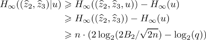
 , which implies
 . Hence, Abort II never happens in this case.
 (resp.
  (resp.
 and
and 
Hence, we get
Observe from the verification algorithm (Algorithm 7) that \(\textbf{A}\textbf{z}^* = u = H(\textsf{msg}, \textsf{salt}, \textsf{vk})\) and \(\Vert \textbf{z}^*\Vert \leqslant B_2\). Also, by the construction of H,
 with
with
 (see \(\textsf{Game} _{3}\)). Consequently, if Abort II does not happen, we can construct an adversary \(\mathcal {B}\) that solves the \(\mathsf {\textsf{RSIS}} _{q,2,2B_2}\) problem for \(\textbf{A}\) since
 for
for
 where \(\textbf{A}= \begin{bmatrix} 1 & a & b \end{bmatrix}\) for a random a (modelling ExpandA as a random oracle) and random b (as discussed in \(\textsf{Game} _{2}\)). More concretely, let \(\textbf{A}= \begin{bmatrix} 1 & a & b \end{bmatrix}\) be the challenge \(\mathsf {\textsf{RSIS}} \) vector given to \(\mathcal {B}\) where \(a,b\overset{\$}{\leftarrow }\mathcal {R}_q\). The adversary \(\mathcal {B}\) samples \(\textsf{seed} \overset{\$}{\leftarrow }\{0,1\}^{\kappa }\) and provides \(\textsf{vk} = (\textsf{seed}, b)\) to \(\mathcal {A} \) against \(\textsf{Game} _{4}\) and programs ExpandA\((\textsf{seed})=a\) (modelling ExpandA as a random oracle). Note that the distribution of \((\textsf{seed}, b)\) matches perfectly the distribution of \(\textsf{vk} \) produced in \(\textsf{Game} _{4}\) due to the change of b in \(\textsf{Game} _{2}\). Since \(\textsf{OSign}\) is run using only with publicly computable values in \(\textsf{Game} _{4}\), \(\mathcal {B}\) simulates \(\textsf{OSign}\) queries as in \(\textsf{Game} _{4}\). \(\mathcal {B}\) also simulates the queries to H as in \(\textsf{Game} _{4}\) and stores the corresponding tables \(\mathcal {T}_H\) and \(\mathcal {T}_s\). As discussed above, provided that Abort II does not happen, \(\mathcal {B}\) can use \(\mathcal {A} \)’s output forgery to create an \(\mathsf {\textsf{RSIS}} _{q,2,2B_2}\) solution. Hence, \(\left| \textsf{Adv} _{\mathcal {B}}^{\mathsf {\textsf{RSIS}}} - \textsf{Adv} _{\mathcal {A}}^{\textsf{Game} _{4}} \right| \leqslant p_c\) and \(T_\mathcal {B}\approx T_\mathcal {A} \). As a result, we get
This concludes the proof.
3.3 Description of Masked \(\mathsf {\mathsf {\textsf{Plover}} \text {-}\mathsf {\textsf{RLWE}} }\)
This section describes our main construction, the masked \(\mathsf {\mathsf {\textsf{Plover}} \text {-}\mathsf {\textsf{RLWE}} }\). \(\mathcal {D}_{\textsf{sk}} \) and \(\mathcal {D}_{\textsf{pert}} \) are respectively replaced by sums of distributions \([d\, \mathsf {\textsf{rep} _\textsf{sk}} ] \cdot \mathcal {D}_{\textsf{sk}}^{\textsf{ind}} \) and \([d\, \mathsf {\textsf{rep} _\textsf{pert}} ] \cdot \mathcal {D}_{\textsf{pert}}^{\textsf{ind}} \) to enable the masking, where \(\mathsf {\textsf{rep} _\textsf{sk}} \) and \(\mathsf {\textsf{rep} _\textsf{pert}} \) are newly introduced parameters.
Key Generation. The key generation generates d-sharings small secrets \(([\![ s ]\!],[\![ e ]\!])\) and the corresponding RLWE sample \(b = a\cdot s +e\). As in Raccoon [29], a key technique is the use of AddRepNoise for the generation of the small errors which ensures that a t-probing adversary learns limited information about (s, e).

Signature Procedure. The signature procedure is adapted to remove the computation of \(z_1\) and save on masking. It recovers \(z_1' = z_1 + c_2\) from unmasked values as done in the verification Algorithm 7 from unmasked values. This also allows to drop e from the private key and significantly reduces its size. A formal description is given in Algorithm 9.

Verification. The verification first recovers \(z'_1 {:}{=}u - az_2 - b z_3 = z_1+c_2\). It then checks the shortness of \((z'_1, z_2, z_3)\). A formal description is given in Algorithm 7.
3.4 Security of Masked \(\mathsf {\mathsf {\textsf{Plover}} \text {-}\mathsf {\textsf{RLWE}} }\)
We now turn to the security of the masked version of \(\mathsf {\textsf{Plover}}\), in the t-probing model. Contrary to proofs for less efficient masking techniques, which have no security loss even in the presence of the probes, we propose a fine-grained result where we quantify precisely the loss induced by the probes and show how the security of this leaky scheme corresponds to the security of the leak-free unmasked \(\mathsf {\textsf{Plover}}\), but with slightly smaller secret key parameters and slightly larger verification norm bound.
Theorem 3
The masked \(\mathsf {\mathsf {\textsf{Plover}} \text {-}\mathsf {\textsf{RLWE}} }\) scheme with parameters \((d, \mathcal {D}_{\textsf{sk}}^{\textsf{ind}} , \mathsf {\textsf{rep} _\textsf{sk}}, \mathcal {D}_{\textsf{pert}}^{\textsf{ind}} , \mathsf {\textsf{rep} _\textsf{pert}}, B_2)\) is t-probing \(\mathsf {\textsf{EUF} \text {-}\textsf{CMA}}\) secure in the random oracle model if the unmasked \(\mathsf {\mathsf {\textsf{Plover}} \text {-}\mathsf {\textsf{RLWE}} } \) scheme with parameters \((\mathcal {D}_{\textsf{sk}},\mathcal {D}_{\textsf{pert}}, B'_2)\) is \(\mathsf {\textsf{EUF} \text {-}\textsf{CMA}}\) secure in the random oracle model, with
where \(B_{\textsf{pert}}\) and \(B_{\textsf{sk}}\) denote upper bounds on the \(\ell _2\) norm of samples from \(\mathcal {D}_{\textsf{pert}}^{\textsf{ind}} \) and \(\mathcal {D}_{\textsf{sk}}^{\textsf{ind}} \), respectively. \(B'_2\) is the norm bound used by the unmasked \(\mathsf {\mathsf {\textsf{Plover}} \text {-}\mathsf {\textsf{RLWE}} }\).
Formally, let \(\mathcal {A} \) denote an adversary against the t-probing \(\mathsf {\textsf{EUF} \text {-}\textsf{CMA}}\) security game against masked \(\mathsf {\mathsf {\textsf{Plover}} \text {-}\mathsf {\textsf{RLWE}} } \) making at most \(Q_{\textsf{Sign}}\) signing queries and at most \(Q_H\) random oracle queries and advantage \(\textsf{Adv} _{\mathcal {A}}^{\mathsf {\textsf{pr} \text {-}\textsf{EUF} \text {-}\textsf{CMA}}}\). Then, there exists an adversary \(\mathcal {A} '\) against \(\mathsf {\textsf{EUF} \text {-}\textsf{CMA}}\) security of unmasked \(\mathsf {\mathsf {\textsf{Plover}} \text {-}\mathsf {\textsf{RLWE}} } \), running in time \(T_{\mathcal {A} '} \approx T_{\mathcal {A}}\) and making \(Q_{\textsf{Sign}}' = Q_{\textsf{Sign}}\) sign queries and \(Q_{H'} = Q_H\) random oracle queries with advantage \(\textsf{Adv} _{\mathcal {A} '}^{\mathsf {\textsf{EUF} \text {-}\textsf{CMA}}}\) such that:
Proof
We describe the reduction with several hybrid games starting from the t-probing \(\mathsf {\textsf{EUF} \text {-}\textsf{CMA}}\) game played with adversary \(\mathcal {A} \) against the masked signature with random oracle H and ending with a game where we can build an adversary \(\mathcal {A} '\) against the \(\mathsf {\textsf{EUF} \text {-}\textsf{CMA}}\) security for the unmasked signature with a random oracle \(H'\). In this and the following games we let \(S_i\) denote the event that \(\mathcal {A} \) wins the t-probing \(\mathsf {\textsf{EUF} \text {-}\textsf{CMA}}\) game.
\({\textsf{Game} _{0}.}\) This corresponds to the t-probing \(\mathsf {\textsf{EUF} \text {-}\textsf{CMA}}\) unforgeability game [5] played with adversary \(\mathcal {A}\). At the beginning of the game, \(\mathcal {A} \) outputs a key gen. probing set \(P_{\textrm{KG}}\) of size \(\leqslant t\), then a masked key generation oracle \(\textsf{OKG}\) runs \(\textsf{MaskKeygen} (1^\kappa )\) to output \((\textsf{vk} {:}{=}(\textsf{seed}, b), \textsf{sk} {:}{=}(\textsf{vk}, [\![ s ]\!]))\) and \(\mathcal {A} \) is given \((\textsf{vk}, \mathcal {L}_{\textrm{KG}})\), where \(\mathcal {L}_{\textrm{KG}} = \textsf{MaskKeygen} _{P_{\textrm{KG}}}\) denotes the observed values of the t probed variables during the execution of \(\mathsf {\mathsf {\textsf{Plover}} \text {-}\mathsf {\textsf{RLWE}} }.\textsf{MaskKeygen} \) with oracle access to Algorithms 8 and 9 with adversary \(\mathcal {A}\). In addition, the adversary is allowed to probe and learn the values of t variables during each execution of Algorithms 8 and 9.
The adversary gets access to a (masked) signing oracle \(\textsf{OSign}(m, P_S)\), where m is a message and \(P_S\) is a signing probing set of size at most t. The oracle returns \((\textsf{sig}, \mathcal {L}_{S})\) where \(\textsf{sig} \leftarrow \mathsf {\mathsf {\textsf{Plover}} \text {-}\mathsf {\textsf{RLWE}} }.\textsf{MaskSign} (m, \textsf{sk})\) and \(\mathcal {L}_{S}\) is the observed values of the t probed variables during the execution of \(\mathsf {\mathsf {\textsf{Plover}} \text {-}\mathsf {\textsf{RLWE}} }.\textsf{MaskSign} \). Before each such \(\textsf{OSign}\) query, the Refresh\(([\![ s ]\!])\) gadget is called by the challenger to refresh the secret key shares (this challenger-run gadget is not probed by \(\mathcal {A} \)). The adversary can also query the random oracle H for the masked scheme. In this game, queries to the masked random oracle H are answered using an internal random oracle \(H'\) (not accessible directly to \(\mathcal {A} \)). The oracles in this game are similar to those in Fig. 2 but without the highlighted lines that are introduced in the following game. The adversary wins the game if it outputs a valid forgery message/signature pair \((\textsf{msg} ^*,\textsf{sig} ^*)\), where \(\textsf{msg} ^*\) has not been queried to \(\textsf{OSign}\).
\(\textsf{Game} _{1} \) (Fig. 2). In this game, we change the computation of the probed observations \((\mathcal {L}_{\textrm{KG}},\mathcal {L}_{S})\) given to \(\mathcal {A} \), from the actual values to the values simulated by probabilistic polynomial time algorithms \(\textsf{SimKG}(P_{\textrm{KG}}, \mathsf {aux_{\textrm{KG}}})\) and \(\textsf{SimSig}(P_{S}, \mathsf {aux_{\textrm{MS}}})\), respectively. The simulation algorithms simulate the probed values using auxiliary information \(\mathsf {aux_{\textrm{KG}}} \) (resp. \(\mathsf {aux_{\textrm{MS}}} \)) consisting of public values and certain leaked internal values as indicated in the highlighted lines of Fig. 2. The main idea (see Sect. 4.2 of [29] for a similar proof) is that the internal t-probed observations in all the gadgets except AddRepNoise can be simulated without the secret shared inputs, whereas by \(\textsf{SNI} \) with unshared inputs property of AddRepNoise in Lemma 1, only \(\leqslant t\) unshared inputs (captured by the auxiliary values
 and
and
 in the masked key generation and signing algorithms, respectively) suffice to simulate its t-probed observations. Note that \(\textsf{Game} _{1}\) writes \(z_1'\) as \(z_1' = p_1 + c_1 \, e + c_2\) instead of \(z_1' = u - a \, z_2 - b \, z_3\); this is a purely syntactic change, as the two expressions are equal and we assume that the secret key includes the error e.
We construct the simulators \(\textsf{SimKG}\) and \(\textsf{SimSig}\) by composing the outputs of the simulators for each gadget, going from the last gadget to the first gadget, similar to the analysis in [5]. In the following description, we use the following notations: For the i’th gadget in \(\textsf{SimKG}\) (resp.\(\textsf{SimSig}\)), we let \(t_i\) denote the number of probed variables in this i’th gadget and by \(\textsf{aux} _i\) the auxiliary (leaked) information needed to simulate the internal view of the i’th gadget. Simulator \(\textsf{SimKG}\) for the probed observations \(\mathcal {L}_{\textrm{KG}}\) works as follows:
-
1.
The Unmask\(([\![ b ]\!])\) gadget (gadget 3) in \(\mathsf {\mathsf {\textsf{Plover}} \text {-}\mathsf {\textsf{RLWE}} }.\textsf{MaskKeygen} \) is t-\(\textsf{NIo} \) (by Lemma 8 in [5]) with public output b. Hence, the probed observations in Unmask can be simulated by \(\textsf{SimKG}\) using \(\leqslant t_3\) input shares in \([\![ b ]\!]\) and the auxiliary information \(\textsf{aux} _3 := b\).
-
2.
The multiplication gadget \(a \cdot [\![ s ]\!] + [\![ e ]\!]\) (gadget 2) in \(\mathsf {\mathsf {\textsf{Plover}} \text {-}\mathsf {\textsf{RLWE}} }.\textsf{MaskKeygen} \) is computed share-wise and therefore is t-\(\textsf{NI} \). Hence, the probed observations in this gadget can be simulated by \(\textsf{SimKG}\) using \(\leqslant t_2+t_3\) input shares in \([\![ s ]\!], [\![ e ]\!]\).
-
3.
The AddRepNoise gadget in \(\mathsf {\mathsf {\textsf{Plover}} \text {-}\mathsf {\textsf{RLWE}} }.\textsf{MaskKeygen} \) is t-\(\textsf{SNIu} \) with \(d \cdot \textsf{rep} \) unshared inputs
 by Lemma 1. Hence, the probed observations in AddRepNoise can be simulated by \(\textsf{SimKG}\) using \(\leqslant t_1+t_2+t_3 \leqslant t\) leaked unshared inputs
 (i.e. the set of safe (unleaked) unshared inputs of AddRepNoise are denoted by
 ).
).
 by Lemma
  (i.e. the set of safe (unleaked) unshared inputs of
  ).
).Overall, \(\textsf{SimKG}\) can simulate the probed observations in \(P_{\textrm{KG}}\) using auxiliary information
 , as shown in Fig. 2.
Similarly, simulator \(\textsf{SimSig}\) for the probed observations \(\mathcal {L}_{S}\) works as follows:
-
1.
The Unmask\(([\![ z_2 ]\!])\) gadget (gadget 6) in \(\mathsf {\mathsf {\textsf{Plover}} \text {-}\mathsf {\textsf{RLWE}} }.\textsf{MaskSign} \) is t-\(\textsf{NIo} \) (by Lemma 8 in [5]) with public output \(z_2\). Hence, the probed observations in Unmask can be simulated by \(\textsf{SimSig}\) using \(\leqslant t_6\) input shares in \([\![ z_2 ]\!]\) and the auxiliary information \(\textsf{aux} _6 := z_2\).
-
2.
The multiplication gadget \([\![ p_2 ]\!] + c_1 \cdot [\![ s ]\!]\) (gadget 5) in \(\mathsf {\mathsf {\textsf{Plover}} \text {-}\mathsf {\textsf{RLWE}} }.\textsf{MaskSign} \) is t-\(\textsf{NI} \). Hence, the probed observations in this gadget can be simulated by \(\textsf{SimSig}\) using \(\leqslant t_5+t_6 \leqslant t\) input shares in \([\![ p_2 ]\!], [\![ s ]\!]\).
-
3.
The Refresh\(([\![ s ]\!])\) gadget (gadget 4) in \(\mathsf {\mathsf {\textsf{Plover}} \text {-}\mathsf {\textsf{RLWE}} }.\textsf{MaskSign} \) is t-\(\textsf{SNI} \) (by [27]). Hence, the probed observations in this gadget can be simulated by \(\textsf{SimSig}\) using \(\leqslant t_4 \leqslant t\) input shares in \([\![ s ]\!]\) (note that those \(t_4\) input shares in \([\![ s ]\!]\) can be simulated by \(\textsf{SimSig}\) as independent uniformly random shares due to the Refresh\(([\![ s ]\!])\) called by the challenger before each \(\textsf{OSign}\) call).
-
4.
The Unmask\(([\![ w ]\!])\) gadget (gadget 3) in \(\mathsf {\mathsf {\textsf{Plover}} \text {-}\mathsf {\textsf{RLWE}} }.\textsf{MaskSign} \) is t-\(\textsf{NIo} \) (by Lemma 8 in [5]) with public output w. Hence, the probed observations in Unmask can be simulated by \(\textsf{SimSig}\) using \(\leqslant t_3\) input shares in \([\![ w ]\!]\) and the auxiliary information \(\textsf{aux} _3 := w\).
-
5.
The multiplication gadget \([\![ p_1 ]\!] + a \cdot [\![ p_2 ]\!]\) (gadget 5) in \(\mathsf {\mathsf {\textsf{Plover}} \text {-}\mathsf {\textsf{RLWE}} }.\textsf{MaskSign} \) is t-\(\textsf{NI} \). Hence, the probed observations in this gadget can be simulated by \(\textsf{SimSig}\) using \(\leqslant t_2+t_3 \leqslant t\) input shares in \([\![ p_1 ]\!], [\![ p_2 ]\!]\).
-
6.
The AddRepNoise gadget (gadget 1) in \(\mathsf {\mathsf {\textsf{Plover}} \text {-}\mathsf {\textsf{RLWE}} }.\textsf{MaskSign} \) is t-\(\textsf{SNI} \) with \(d \cdot \textsf{rep} \) unshared inputs
 by Lemma 4. Hence, the probed observations in AddRepNoise can be simulated by \(\textsf{SimSig}\) using \(\leqslant t_1 \leqslant t\) leaked unshared inputs
 (i.e. the set of safe (unleaked) unshared inputs of AddRepNoise are denoted by
 ).
).
 by Lemma
  (i.e. the set of safe (unleaked) unshared inputs of
  ).
).Overall, \(\textsf{SimSig}\) can simulate the probed observations in \(P_{S}\) using auxiliary information
 , as shown in Fig. 2. (note that \(\textsf{aux} _3 = w\) can be computed from \(\mathsf {aux_{\textrm{MS}}} \) since \(w = u - c\), \(u=H(\textsf{msg},\textsf{salt},\textsf{vk})\) with \(\textsf{salt} \) taken from \(\textsf{sig} \), and c computed from \(c_1\) in \(\textsf{sig} \) and \(c_2\) in \(\mathsf {aux_{\textrm{sig}}} \)).

Algorithms in \(\textsf{Game} _{1}\)
Since the view of \(\mathcal {A} \) is perfectly simulated in this game as in the previous game, we have \(\Pr [S_1]=\Pr [S_0]\).
\(\textsf{Game} _{2} \) (Fig. 3). In this game, we re-arrange the computation in \(\textsf{OKG}\) to first compute a ‘safe’ verification key
 using the ‘safe’ part
 of the secret key, and only later sample the ‘leaked’ part
 of the secret key and use this leaked secret and
 to compute the full verification key
 . The above change to \(\textsf{OKG}\) is just a re-ordering of the computation and thus does not change the view of \(\mathcal {A} \).
In this game, we also similarly re-arrange the computation in \(\textsf{OSign}\) to first compute a ‘safe’ part of the signature
 with
with
 , using the ‘safe’ perturbation part
 and ‘safe secret key part
 , and later compute the full signature \(\textsf{sig} \) from the
 by adding the ‘leaked’ signature part to get
 , where the last equality holds if
 . Hence, for this re-arranged computation to preserve the correctness of the final signature (in particular \(z_2\)) as in the previous game (and thus preserve \(\mathcal {A} \)’s view), we need to ensure that
 in the top ‘safe’ part of the computation, is equal to \(c {:}{=}u - w\) used in the bottom ‘leaked’ part of the computation. To achieve this, we use the random oracle \(H'\) (not directly accessible to \(\mathcal {A} \)) to compute
 in the ‘safe’ part of the computation, and we change the simulation of the random oracle H accessible to \(\mathcal {A} \) by programming H so that
 , where
 is sampled by the simulation and stored in the table \(\mathcal {T}_H\) for H. Defining
 , we have
 , as required.
Since
 is uniformly random in \(R_q\) and independent of
 , the simulation of H is identical to the previous game from \(\mathcal {A} \)’s view, except if an abort happens in \(\textsf{OSign}\) line 18 (we say then that the event \(B_2\) occurs). However, since \(\textsf{salt} \) is uniformly random in \(\{0, 1\}^{2 \kappa } \) for each sign query, the event \(B_2\) occurs with negligible probability \(\Pr [B_2] \leqslant Q_{\textsf{Sign}}Q_H / 2^{2\kappa }\). Therefore, overall we have \(\Pr [S_2] \geqslant \Pr [S_1] - \Pr [B_2] \geqslant \Pr [S_1]- Q_{\textsf{Sign}}Q_H/2^{2\kappa }\).

Algorithms in \(\textsf{Game} _{2}\)
We now construct an adversary \(\mathcal {A} '\) against the \(\mathsf {\textsf{EUF} \text {-}\textsf{CMA}}\) of the unmasked signature scheme \(\textsf{Sign} \) with random oracle \(H'\), secret key distribution \(\mathcal {D}_{\textsf{sk}}:= [d \, \mathsf {\textsf{rep} _\textsf{sk}}- t] \cdot \mathcal {D}_{\textsf{sk}}^{\textsf{ind}} \), and perturbation distribution \(\mathcal {D}_{\textsf{pert}}:= [d \, \mathsf {\textsf{rep} _\textsf{pert}}- t] \cdot \mathcal {D}_{\textsf{pert}}^{\textsf{ind}} \) that simulates view of \(\mathcal {A} \) in \(\textsf{Game} _{2}\), such that \(\mathcal {A} '\) wins its game with probability \(\geqslant \Pr [S_2]\). The challenger for \(\mathcal {A} '\) generates a challenge key pair
 by running lines 1–6 of \(\textsf{OKG}\) in \(\textsf{Game} _{2}\) (this corresponds exactly to the key gen. algorithm for the unmasked scheme) and runs \(\mathcal {A} '\) on input \(\textsf{vk} '\). Then \(\mathcal {A} '\) runs as follows.
-
1.
It first runs \(\mathcal {A} \) to get \(P_{\textrm{KG}}\) and then runs lines 7–12 of \(\textsf{OKG}\) in \(\textsf{Game} _{2} \) to get \((\textsf{vk}, \textsf{sk}, \mathcal {L}_{\textrm{KG}})\) and runs \(\mathcal {A} \) on input \((\textsf{vk}, \mathcal {L}_{\textrm{KG}})\).
-
2.
Similarly, to respond to each \(\textsf{OSign}\) query \((\textsf{msg}, P_S)\) of \(\mathcal {A} \), \(\mathcal {A} '\) calls its \(\textsf{Sign} \) algorithm on input \(\textsf{msg} \) (this corresponds to running lines 1–11 of \(\textsf{OKG}\) in \(\textsf{Game} _{2}\)), and using the returned
 and
and
 , \(\mathcal {A} '\) runs lines 12–26 of \(\textsf{OSign}\) in \(\textsf{Game} _{2}\) to compute and return \((\textsf{sig}, \mathcal {L}_{S})\) to \(\mathcal {A} \) (note that
 is computed by \(\mathcal {A} '\) from
 and
and
 obtained from \(c_1\) in
 and \(c_2\) in
 ).
). -
3.
\(\mathcal {A} '\) also runs the H simulator in \(\textsf{Game} _{2} \) to respond to \(\mathcal {A} \)’s H queries, where \(H'\) is the random oracle provided to \(\mathcal {A} '\) by its challenger.
 and
and
 ,
,  is computed by
  and
and
 obtained from
  and
and  ).
).Consequently, the view of \(\mathcal {A} \) is perfectly simulated as in \(\textsf{Game} _{2}\), so with probability \(\Pr [S_2]\), \(\mathcal {A} \) outputs a valid forgery \((\textsf{msg} ^*,\textsf{sig} ^*=(\textsf{salt} ^*,z_2^*,c_1^*))\) such that \(\Vert (z_1'^*,z_2^*,z_3^*)\Vert \leqslant B_2\), and \(\Vert c_1^*\Vert _{\infty } \leqslant q/(2\beta )+1/2\) and \(z_1'^* + a z_2^* + b c_1^* = u^* = H(\textsf{msg} ^*,\textsf{salt} ^*,\textsf{vk})\) where \(\textsf{msg} ^*\) has not been queried by \(\mathcal {A} \) to \(\textsf{OSign}\). Then, \(\mathcal {A} '\) computes
 with
with
 and returns its forgery
 , where
 .
.
Note that, defining
 and
and
 (where
 is obtained from \(\mathcal {T}_H\) entry for the forgery H-query \((\textsf{msg} ^*,\textsf{salt} ^*,\textsf{vk})\)), we have
 and so forgery
 satisfies the unmasked scheme validity relation
 , as required. Also,
 , since
 . Finally, \(\textsf{msg} ^*\) has not been queried by \(\mathcal {A} '\) to its unmasked signing oracle. It follows that \(\mathcal {A} '\) wins with probability \(\geqslant \Pr [S_2] \geqslant \Pr [S_0] - Q_{\textsf{Sign}}Q_H / 2^{2\kappa }\). This concludes the proof.
3.5 Cryptanalysis and Parameter Selection
Now that the security of our scheme is formally proven in unmasked form for general distributions \(\mathcal {D}_{\textsf{sk}},\mathcal {D}_{\textsf{pert}} \) and the security of the masked form reduces to its unmasked form, we wish to demonstrate concrete parameter selection for masked \(\mathsf {\mathsf {\textsf{Plover}} \text {-}\mathsf {\textsf{RLWE}} }\). We evaluate the concrete security of our scheme against \(\mathsf {\textsf{RSIS}}\) for forgery, and against \(\mathsf {\textsf{Hint} \text {-}\mathsf {\textsf{RLWE}}}\) for key-indistinguishability using the reduction from \(\mathsf {\textsf{Hint} \text {-}\mathsf {\textsf{RLWE}}}\) to \(\mathsf {\textsf{RLWE}}\) (Theorem 1) and standard evaluation heuristics.
Optimizations. For our implementation, we use these standard optimizations:
-
Norm check. We add a norm check in \(\textsf{MaskSign} \) against \(B_2\), allowing to reject with low probability some large signatures, and making forgery harder. Note that this is not rejection sampling, and it can be done unmasked.
-
Bit-dropping. We can drop the \(\mathsf {\nu } \) least significant bits of b. More formally, let us note \((b_1, b_2) =\) Decompose\(_{\{ 2^\mathsf {\nu } \}}(b)\) where \(\mathsf {\nu } \) is the number of bits dropped in each coefficient of b. We can set \(2^\mathsf {\nu } \cdot b_1\) as a public key.
As long as \(\mathsf {\nu } = O \left( \log \left( \frac{\sigma _\textsf{pert} ^2}{q \sqrt{n}} \right) \right) \), we can show that breaking inhomogeneous \(\mathsf {\textsf{RSIS}}\) for \(\begin{bmatrix} 1 & a & 2^\mathsf {\nu } \cdot b_1 \end{bmatrix}\) implies breaking it for \(\begin{bmatrix} 1 & a & b \end{bmatrix}\) with comparable parameters. This reduces the size of \(\textsf{vk}\), while preserving the security reduction.
Forgery Attacks and Practical RSIS Security. Let \(\sigma _\textsf{sk}, \sigma _\textsf{pert} \) denote the standard deviation of the (unmasked) secret key and perturbation, respectively. In a legitimate signature:
Based on this analysis, we set \(B_2= 1.2 \, \sqrt{ n \left( 2 \, \sigma _\textsf{pert} ^2 + \frac{\beta ^2}{12} + \frac{q^2 \, n}{6 \, \beta ^2 } \, \sigma _\textsf{sk} ^2 + n\frac{2^{2\mathsf {\nu }}}{12} \frac{q^2}{12\beta ^2} \right) }\). The “slack” factor 1.2 allows an extremely large number of generated signatures to satisfy \(\left\| \textbf{z}'\right\| \leqslant B_2\), which means that the restart rate will be very low.
Solving Inhomogeneous \(\mathsf {\textsf{RSIS}}\) . To forge a message, an adversary must either break the collision resistance of H or solve the equation:
Note that \(\begin{bmatrix} 1 & a & \beta \cdot b_1 \end{bmatrix} \cdot \textbf{z}' = \begin{bmatrix} 1 & a & b \end{bmatrix} \cdot \textbf{z}''\), where \(\textbf{z}'' = \textbf{z}' - (z_3 \cdot b_2, 0, 0)\), and that \(\left\| z_3 \cdot b_2\right\| \leqslant \left\| c_1\right\| _1 \cdot \left\| b_2\right\| \leqslant n^{3/2} \cdot \frac{q \, 2^{\mathsf {\nu }- 2}}{\beta } \). Then Eq. (3) is an instance of the inhomogeneous \(\mathsf {\textsf{RSIS}}\) problem, with a bound \(B_{\mathsf {\textsf{RSIS}}}= B_2+ n^{3/2} \cdot \frac{q \, 2^{\mathsf {\nu }- 2}}{\beta }\).
We estimate its hardness based on Chuengsatiansup et al. [9] and Espitau and Kirchner [15]. Under the geometric series assumption, [15, Theorem 3.3] states that Eq. (3) can be solved in \(\textsf{poly} (n)\) calls to a CVP oracle in dimension \(B_{\textsf{BKZ}}\), as long as:
This attack has been optimized in [9] by omitting \(x \leqslant n\) of the first columns of \(\textbf{A}\) (when considered as a \(n \times 3 \, n\) matrix). The dimension is reduced by x, however, the co-volume of the lattice is increased to \(q^{\frac{ n }{ 3 n - x}}\). This strengthens Eq. (4) to the more stringent condition \( B_{\mathsf {\textsf{RSIS}}}\leqslant \min _{x \leqslant n} \left( \delta _{B_{\mathsf {\textsf{RSIS}}}}^{ 3 n - x }q^{\frac{n}{3 n - x}} \right) .\)
Key-Indistinguishability and Hint-RLWE. In order to apply Theorem 1, we need quantitative bounds on \(B_{\textsf{HRLWE}}\). These are given in Lemma 2, which is a minor adaptation of [30, Lemma B.2]. A proof is provided in the full version for completeness.
Lemma 2
For \(j \in [Q_{\textsf{Sign}}]\), let \(c^{[j]} \leftarrow \mathcal {C} _1\), where \(\mathcal {C} _1\) is defined as in Definition 9. Let \(D = \sum _{j \in [Q_{\textsf{Sign}}]} c^{[j]} \, ( c^{[j]} )^*\). Let \(M = 2 \left\lceil \frac{q - 1}{2 \beta } \right\rceil + 1\). We then have \(\Pr \left[ s_1(D) \geqslant B_{\textsf{HRLWE}}\right] \le 2^{-\kappa }\), where \( B_{\textsf{HRLWE}}= \frac{Q_{\textsf{Sign}}\, n \, M^2 }{12} \left( 1 + \frac{ O(\kappa \, n \log n) }{ \sqrt{Q_{\textsf{Sign}}} }\right) \). Specifically, when \(Q_{\textsf{Sign}}= \omega (\kappa \, n \log n)^2\), then \(s_1(D)\) is equivalent to \(\frac{Q_{\textsf{Sign}}\, n \, M^2 }{12}\).
Advantage Against \(\mathsf {\textsf{Hint} \text {-}\mathsf {\textsf{RLWE}}} \). An adversary breaking the key-indistinguishability of \(\textsf{vk}\) is also able to break
 . In the Gaussian case,
 and
and
 , where
 .
.
Theorem 1 and Lemma 2 state that such an adversary is also able to break \(\mathsf {\textsf{RLWE}} _{q, D_{\sigma _\textsf{red}}}\), where
 and \(B_{\textsf{HRLWE}}\) is as in Lemma 2. For the parameters we choose in practice, this entails:
 Estimating the concrete hardness of \(\mathsf {\textsf{RLWE}}\) is well-documented. We rely on the lattice estimator [2], an open-source tool available at https://github.com/malb/lattice-estimator.
Parameter Selection. Despite the many variables involved, parameter selection is fairly straightforward. We set \(\beta = \varTheta (\sigma _\textsf{pert})\), \(\mathsf {\nu } = \varTheta \left( \log \left( \frac{\sigma _\textsf{pert} ^2}{q \sqrt{n}} \right) \right) \) and \(\sigma _\textsf{sk} = o \left( \frac{\beta \, \sigma _\textsf{pert}}{q \sqrt{n}} \right) \). This guarantees efficiency while ensuring that \(B_{\mathsf {\textsf{RSIS}}}= O(\sigma _\textsf{pert} \sqrt{n})\).

Illustration of the constraints on q (in log scale): \(\mathsf {\textsf{RSIS}}\) and \(\mathsf {\textsf{RLWE}}\) must be hard, and the \(\mathsf {\textsf{Hint} \text {-}\mathsf {\textsf{RLWE}}} \geqslant \mathsf {\textsf{RLWE}} \) reduction must be non-vacuous.
These parameters also guarantee an efficient reduction in Theorem 1. We estimate the number of queries, \(Q_{\textsf{Sign}}\), by increasing it for as long as the \(\mathsf {\textsf{RLWE}}\) instance entailed by the reduction of Theorem 1 and Lemma 2 remains secure according to the state-of-the-art. \(Q_{\textsf{Sign}}'\) corresponds to the number of queries allowed when the condition \(\sigma \geqslant \sqrt{2} \eta _{\varepsilon }(\mathbb {Z}^n)\) is dropped in Theorem 1.
We illustrate constraints over the modulo q in Fig. 4. Selected parameters are provided in Table 1, and the evolution of allowed number of queries as a function of \(\log q\) is illustrated in Fig. 5.
3.6 Implementation
We provide both a Python and a C reference implementation for \(\mathsf {\mathsf {\textsf{Plover}} \text {-}\mathsf {\textsf{RLWE}} }\), available at https://github.com/GuilhemN/masksign-plover. They are designed to match the high-level pseudo-code from Subsect. 3.3 and allows one to read a concrete implementation of each of the functions we introduced. The Python implementation aims for simplicity and is not constant-time, while the C implementation is constant-time and uses optimization techniques. We include scripts for parameters selection under the folder params based on the lattice estimator [2].

Number of signing queries (conservative:
 , standard:
 ) and bytesizes (\(|\textsf{vk} |\):
 , \(|\textsf{sig} |\):
 ) as functions of q. Parameter sets as in Sect. 3.5.

 ,
,  ) as functions of d. Parameter set from Sect.
 These reference implementations re-use several components of \(\textsf{Raccoon}\) reference implementations [29] for the NTT, Montgomery modular reduction, and randomness generators. They are portable and can target various masking orders \(d-1\). Note however that they suffer from the same issues as \(\textsf{Raccoon}\) reference implementations. Specifically, a deterministic portable code written in a high-level language cannot realistically be considered to be fully resistant to side-channel attacks, and notably due to the use of the randombytes function defined by NIST, which represents an abstract RBG (Random Bit Generator), but is only suitable to ease reproducibility and generation of test vectors. Additionally, our reference implementations are severely limited in their key management as the NIST API does not allow for a refresh of the secret key, which is required for t-probing security. We argue that these implementations still provide evidence that \(\mathsf {\mathsf {\textsf{Plover}} \text {-}\mathsf {\textsf{RLWE}} }\) is easy to mask at high masking orders.
General Implementation Characteristics. \(\mathsf {\mathsf {\textsf{Plover}} \text {-}\mathsf {\textsf{RLWE}} }\) has building blocks resembling those of \(\textsf{Raccoon}\) [29], as well as a modulus q of same magnitude and format (product of two Solinas primes). In particular we reuse part of their codebase and of their implementation tricks.
Signature Encoding. We encode low-order bits using binary encoding, and high-order bits using Huffman/unary-type encoding. This encoding is similar to the ones in Falcon and \(\textsf{Raccoon}\). We chose this technique over ANS encoding – although ANS could compress signatures further – as the latter proved hard to implement securely in NIST Call for Additional Digital Signature Schemes, with vulnerabilities discovered in the HuFu and HAETAE proposalsFootnote 1.
Mask Compression Technique. Our implementation uses the mask compression technique introduced in [29, 33] in order to reduce the size of the stored secret key, which contains the masked polynomial \([\![ s ]\!]\). A masked polynomial at order d can be compressed into one polynomial and \(d-1\) seeds which can be later expanded into full polynomial masking shares. We refer to [29, Algorithms 14 and 15] and [33] for a detailed specification of this technique.
This technique could also be used to drastically reduce the memory requirements of \(\mathsf {\mathsf {\textsf{Plover}} \text {-}\mathsf {\textsf{RLWE}} }\). Our masking gadgets can be adapted to do runtime computations on compressed masked polynomials to limit the impact of a larger d on memory requirements. For reference, \(\textsf{Raccoon}\) [29, section 3.3.2] reduced memory usage for a masking order \(d=32\) by a factor of 15 using this technique.
Hardware. \(\mathsf {\mathsf {\textsf{Plover}} \text {-}\mathsf {\textsf{RLWE}} }\) could be implemented on hardware in a similar manner to Raccoon. Several versions of Raccoon were implemented on FPGA architecture, one is reported in [31]. These implementations contain a RISC-V controller, a Keccak accelerator, and a lattice unit with direct memory access via a 64-bit interface, using hard-coded support for Raccoon’s arithmetic modulus q. \(\mathsf {\mathsf {\textsf{Plover}} \text {-}\mathsf {\textsf{RLWE}} }\) can share a large part of these implementations.
As for Raccoon [29, section 3.3.1] the usage of SHAKE as hash function in the implementation of ExpandA and AddRepNoise can be highly optimized in hardware, and the hardware XOF (eXtendable-Output Functions) sampler can implement a full Keccak round and produce output at a very high rate.
Performance. We evaluated the performance of \(\mathsf {\mathsf {\textsf{Plover}} \text {-}\mathsf {\textsf{RLWE}} }\) on a Ryzen Pro 7 5850U (16CPU threads at 3 GHz), boost disabled, and running Manjaro 22.1. The results are provided in Table 2 and Fig. 6. The reference implementation instantiates the parameter set from Table 1 such that \(\lceil \log q\rceil = 41\), as it is optimal for the number of possible queries for \(n=2048\) and \(\kappa =128\). Other parameter sets perform very similarly since – performance-wise – only the encoding differs between them. The implementation packages parameters for d shares, \(d\in \{1, 2, 4, 8, 16, 32\}\), and the distributions \(\mathcal {D}_{\textsf{sk}} \) and \(\mathcal {D}_{\textsf{pert}} \) are sums of uniforms \(\textsc {SU}(u_\textsf{sk}, d\cdot \mathsf {\textsf{rep} _\textsf{sk}}) \) and \(\textsc {SU}(u_\textsf{pert}, d\cdot \mathsf {\textsf{rep} _\textsf{pert}}) \) with \(\textsf{rep}:= \mathsf {\textsf{rep} _\textsf{sk}} = \mathsf {\textsf{rep} _\textsf{pert}} \in \{2, 4, 8\}\) a function of d. \(u_\textsf{sk} \) and \(u_\textsf{pert} \) are chosen as to achieve a standard deviation close to \(\sigma _\textsf{sk} \) and \(\sigma _\textsf{pert} \). \(\mathsf {\mathsf {\textsf{Plover}} \text {-}\mathsf {\textsf{RLWE}} }\) has performance very similar to \(\textsf{Raccoon}\); in particular, we observe a (quasi-)linear increase in the execution times and stack usage of our functions with d, which makes the use of a high masking order practical. For instance, \(\mathsf {\mathsf {\textsf{Plover}} \text {-}\mathsf {\textsf{RLWE}} }\) masked with a number of shares \(d=8\) still performs better than Dilithium masked with \(d=2\) [29, Table 6].
References
Alagic, G., et al.: NISTIR 8413 – Status Report on the Third Round of the NIST Post-Quantum Cryptography Standardization Process (2022). https://doi.org/10.6028/NIST.IR.8413
Albrecht, M.R., Player, R., Scott, S.: On the concrete hardness of learning with errors. J. Math. Cryptol. 9(3), 169–203 (2015). http://www.degruyter.com/view/j/jmc.2015.9.issue-3/jmc-2015-0016/jmc-2015-0016.xml
Azouaoui, M., et al.: Protecting dilithium against leakage revisited sensitivity analysis and improved implementations. IACR Trans. Cryptogr. Hardw. Embed. Syst. 2023(4), 58–79 (2023). https://doi.org/10.46586/tches.v2023.i4.58-79
Barthe, G., et al.: Strong non-interference and type-directed higher-order masking. In: Weippl, E.R., Katzenbeisser, S., Kruegel, C., Myers, A.C., Halevi, S. (eds.) ACM CCS 2016, pp. 116–129. ACM Press, October 2016. https://doi.org/10.1145/2976749.2978427
Barthe, G., et al.: Masking the GLP lattice-based signature scheme at any order. In: Nielsen, J.B., Rijmen, V. (eds.) EUROCRYPT 2018. LNCS, vol. 10821, pp. 354–384. Springer, Cham (2018). https://doi.org/10.1007/978-3-319-78375-8_12
Battistello, A., Coron, J.-S., Prouff, E., Zeitoun, R.: Horizontal side-channel attacks and countermeasures on the ISW masking scheme. In: Gierlichs, B., Poschmann, A.Y. (eds.) CHES 2016. LNCS, vol. 9813, pp. 23–39. Springer, Heidelberg (2016). https://doi.org/10.1007/978-3-662-53140-2_2
Berzati, A., Viera, A.C., Chartouny, M., Madec, S., Vergnaud, D., Vigilant, D.: Exploiting intermediate value leakage in dilithium: a template-based approach. IACR Trans. Cryptogr. Hardw. Embed. Syst. 2023(4), 188–210 (2023). https://doi.org/10.46586/tches.v2023.i4.188-210
Bronchain, O., Cassiers, G.: Bitslicing arithmetic/boolean masking conversions for fun and profit with application to lattice-based KEMs. IACR TCHES 2022(4), 553–588 (2022). https://doi.org/10.46586/tches.v2022.i4.553-588
Chuengsatiansup, C., Prest, T., Stehlé, D., Wallet, A., Xagawa, K.: ModFalcon: Compact signatures based on module-NTRU lattices. In: Sun, H.M., Shieh, S.P., Gu, G., Ateniese, G. (eds.) ASIACCS 2020, pp. 853–866. ACM Press, October 2020. https://doi.org/10.1145/3320269.3384758
Coron, J., Gérard, F., Montoya, S., Zeitoun, R.: High-order polynomial comparison and masking lattice-based encryption. IACR Trans. Cryptogr. Hardw. Embed. Syst. 2023(1), 153–192 (2023). https://doi.org/10.46586/tches.v2023.i1.153-192
Coron, J., Gérard, F., Trannoy, M., Zeitoun, R.: High-order masking of NTRU. IACR Trans. Cryptogr. Hardw. Embed. Syst. 2023(2), 180–211 (2023). https://doi.org/10.46586/tches.v2023.i2.180-211
Coron, J., Gérard, F., Trannoy, M., Zeitoun, R.: Improved gadgets for the high-order masking of dilithium. IACR Trans. Cryptogr. Hardw. Embed. Syst. 2023(4), 110–145 (2023). https://doi.org/10.46586/tches.v2023.i4.110-145
Duc, A., Faust, S., Standaert, F.X.: Making masking security proofs concrete (or how to evaluate the security of any leaking device), extended version. J. Cryptol. 32(4), 1263–1297 (2019). https://doi.org/10.1007/s00145-018-9277-0
Espitau, T., Fouque, P.A., Gérard, F., Rossi, M., Takahashi, A., Tibouchi, M., Wallet, A., Yu, Y.: Mitaka: A simpler, parallelizable, maskable variant of falcon. In: Dunkelman, O., Dziembowski, S. (eds.) EUROCRYPT 2022, Part III. LNCS, vol. 13277, pp. 222–253. Springer, Heidelberg (May / Jun 2022). https://doi.org/10.1007/978-3-031-07082-2_9
Espitau, T., Kirchner, P.: The nearest-colattice algorithm. Cryptology ePrint Archive, Report 2020/694 (2020). https://eprint.iacr.org/2020/694
Gentry, C., Peikert, C., Vaikuntanathan, V.: Trapdoors for hard lattices and new cryptographic constructions. In: Ladner, R.E., Dwork, C. (eds.) 40th ACM STOC, pp. 197–206. ACM Press, May 2008. https://doi.org/10.1145/1374376.1374407
Goldwasser, S., Kalai, Y.T., Peikert, C., Vaikuntanathan, V.: Robustness of the learning with errors assumption. In: Yao, A.C. (ed.) Innovations in Computer Science - ICS 2010, Tsinghua University, Beijing, China, 5–7 January 2010. Proceedings, pp. 230–240. Tsinghua University Press (2010). http://conference.iiis.tsinghua.edu.cn/ICS2010/content/papers/19.html
Goubin, L.: A sound method for switching between Boolean and arithmetic masking. In: Koç, Ç.K., Naccache, D., Paar, C. (eds.) CHES 2001. LNCS, vol. 2162, pp. 3–15. Springer, Heidelberg (2001). https://doi.org/10.1007/3-540-44709-1_2
Guerreau, M., Martinelli, A., Ricosset, T., Rossi, M.: The hidden parallelepiped is back again: Power analysis attacks on falcon. IACR TCHES 2022(3), 141–164 (2022). https://doi.org/10.46586/tches.v2022.i3.141-164
Ishai, Y., Sahai, A., Wagner, D.: Private circuits: securing hardware against probing attacks. In: Boneh, D. (ed.) CRYPTO 2003. LNCS, vol. 2729, pp. 463–481. Springer, Heidelberg (2003). https://doi.org/10.1007/978-3-540-45146-4_27
Ito, A., Ueno, R., Homma, N.: On the success rate of side-channel attacks on masked implementations: information-theoretical bounds and their practical usage. In: Yin, H., Stavrou, A., Cremers, C., Shi, E. (eds.) ACM CCS 2022, pp. 1521–1535. ACM Press, November 2022. https://doi.org/10.1145/3548606.3560579
Kannwischer, M.J., Genêt, A., Butin, D., Krämer, J., Buchmann, J.: Differential power analysis of XMSS and SPHINCS. In: Fan, J., Gierlichs, B. (eds.) COSADE 2018. LNCS, vol. 10815, pp. 168–188. Springer, Cham (2018). https://doi.org/10.1007/978-3-319-89641-0_10
Karabulut, E., Alkim, E., Aysu, A.: Single-trace side-channel attacks on \(\omega \)-small polynomial sampling: with applications to NTRU, NTRU prime, and CRYSTALS-DILITHIUM. In: IEEE International Symposium on Hardware Oriented Security and Trust, HOST 2021, Tysons Corner, VA, USA, 12–15 December 2021, pp. 35–45. IEEE (2021). https://doi.org/10.1109/HOST49136.2021.9702284
Kim, D., Lee, D., Seo, J., Song, Y.: Toward practical lattice-based proof of knowledge from hint-MLWE. In: Handschuh, H., Lysyanskaya, A. (eds.) CRYPTO 2023, Part V. LNCS, vol. 14085, pp. 549–580. Springer, Heidelberg (2023). https://doi.org/10.1007/978-3-031-38554-4_18
Kim, M., Lee, D., Seo, J., Song, Y.: Accelerating HE operations from key decomposition technique. In: Handschuh, H., Lysyanskaya, A. (eds.) CRYPTO 2023, Part IV. LNCS, vol. 14084, pp. 70–92. Springer, Heidelberg (2023). https://doi.org/10.1007/978-3-031-38551-3_3
Masure, L., Rioul, O., Standaert, F.: A nearly tight proof of Duc et al.’s conjectured security bound for masked implementations. In: Buhan, I., Schneider, T. (eds.) CARDIS 2022. LNCS, vol. 13820, pp. 69–81. Springer, Cham (2022). https://doi.org/10.1007/978-3-031-25319-5_4
Mathieu-Mahias, A.: Securisation of implementations of cryptographic algorithms in the context of embedded systems. Theses, Université Paris-Saclay, December 2021. https://theses.hal.science/tel-03537322
Montgomery, P.L.: Speeding the pollard and elliptic curve methods of factorization. Math. Comput. 48(177), 243–264 (1987). https://doi.org/10.1090/s0025-5718-1987-0866113-7
del Pino, R., et al.: Raccoon, a side-channel secure signature scheme. Technical report. National Institute of Standards and Technology (2023). https://csrc.nist.gov/Projects/pqc-dig-sig/round-1-additional-signatures
del Pino, R., Katsumata, S., Maller, M., Mouhartem, F., Prest, T., Saarinen, M.J.: Threshold raccoon: practical threshold signatures from standard lattice assumptions. Cryptology ePrint Archive, Paper 2024/184 (2024). https://eprint.iacr.org/2024/184
del Pino, R., Prest, T., Rossi, M., Saarinen, M.O.: High-order masking of lattice signatures in quasilinear time. In: 44th IEEE Symposium on Security and Privacy, SP 2023, San Francisco, CA, USA, 21–25 May 2023, pp. 1168–1185. IEEE (2023). https://doi.org/10.1109/SP46215.2023.10179342
Prest, T.: A key-recovery attack against Mitaka in the \(t\)-probing model. In: Boldyreva, A., Kolesnikov, V. (eds.) PKC 2023, Part I. LNCS, vol. 13940, pp. 205–220. Springer, Heidelberg (2023). https://doi.org/10.1007/978-3-031-31368-4_8
Saarinen, M.J.O., Rossi, M.: Mask compression: high-order masking on memory-constrained devices. Cryptology ePrint Archive, Paper 2023/1117 (2023). https://eprint.iacr.org/2023/1117
Yu, Y., Jia, H., Wang, X.: Compact lattice gadget and its applications to hash-and-sign signatures. In: Handschuh, H., Lysyanskaya, A. (eds.) CRYPTO 2023, Part V. LNCS, vol. 14085, pp. 390–420. Springer, Heidelberg (2023). https://doi.org/10.1007/978-3-031-38554-4_13
Zhang, S., Lin, X., Yu, Y., Wang, W.: Improved power analysis attacks on falcon. In: Hazay, C., Stam, M. (eds.) EUROCRYPT 2023, Part IV. LNCS, vol. 14007, pp. 565–595. Springer, Heidelberg (2023). https://doi.org/10.1007/978-3-031-30634-1_19
Author information
Authors and Affiliations
Corresponding author
Editor information
Editors and Affiliations
Rights and permissions
Copyright information
© 2024 International Association for Cryptologic Research
About this paper

Cite this paper
Esgin, M.F., Espitau, T., Niot, G., Prest, T., Sakzad, A., Steinfeld, R. (2024). \(\mathsf {\textsf{Plover}}\): Masking-Friendly Hash-and-Sign Lattice Signatures. In: Joye, M., Leander, G. (eds) Advances in Cryptology – EUROCRYPT 2024. EUROCRYPT 2024. Lecture Notes in Computer Science, vol 14657. Springer, Cham. https://doi.org/10.1007/978-3-031-58754-2_12
Download citation
DOI: https://doi.org/10.1007/978-3-031-58754-2_12
Published:
Publisher Name: Springer, Cham
Print ISBN: 978-3-031-58753-5
Online ISBN: 978-3-031-58754-2
eBook Packages: Computer ScienceComputer Science (R0)
