Adaptive Partitioning

Abstract

We present a new strategy for partitioning proofs, and use it to obtain new tightly secure encryption schemes. Specifically, we provide the following two conceptual contributions:

• A new strategy for tight security reductions that leads to compact public keys and ciphertexts.

• A relaxed definition of non-interactive proof systems for non-linear (“OR-type”) languages. Our definition is strong enough to act as a central tool in our new strategy to obtain tight security, and is achievable both in pairing-friendly and DCR groups.

We apply these concepts in a generic construction of a tightly secure public-key encryption scheme. When instantiated in different concrete settings, we obtain the following:

• A public-key encryption scheme whose chosen-ciphertext security can be tightly reduced to the DLIN assumption in a pairing-friendly group. Ciphertexts, public keys, and system parameters contain $6$, $24$, and $2$ group elements, respectively. This improves heavily upon a recent scheme of Gay et al. (Eurocrypt 2016) in terms of public key size, at the cost of using a symmetric pairing.

• The first public-key encryption scheme that is tightly chosen-ciphertext secure under the DCR assumption. While the scheme is not very practical (ciphertexts carry $28$ group elements), it enjoys constant-size parameters, public keys, and ciphertexts.

D. Hofheinz—Supported by DFG grants HO 4534/4-1 and HO 4534/2-2.

1 Introduction

Tight Security. Ideally, the only way to attack a cryptographic scheme $S$ should be to solve a well-investigated, presumably hard computational problem $P$ (such as factoring large integers). In fact, most existing constructions of cryptographic schemes provide such security guarantees, by exhibiting a security reduction. A reduction shows that any attack that breaks the scheme with some probability $\varepsilon _{S}$ implies a problem solver that succeeds with probability $\varepsilon _{P}$. Of course, we would like $\varepsilon _{P}$ to be as large as possible, depending on $\varepsilon _{S}$.

Specifically, we could call the quotient $\ell :=\varepsilon _{S}/\varepsilon _{P}$ the security loss of a reduction.¹ A small value of $\ell$ is desirable, since it indicates a tight coupling of the security of the scheme to the hardness of the computational problem. It is also desirable that $\ell$ does not depend, e.g., on the number of considered instances of the scheme. Namely, when $\ell$ is linear in the number of instances, the scheme’s security guarantees might vanish quickly in large settings. This can be a problem when being forced to choose concrete key sizes for schemes in settings whose size is not even known at setup time.

Hence, let us call a security reduction tight if its security loss $\ell$ only depends on a global security parameter (but not, e.g., on the number of considered instances, or the number of usages). Most existing cryptographic reductions are not tight. Specifically, it appears to be a nontrivial problem to construct tightly secure public-key primitives, such as public-key encryption, or digital signature schemes. (A high-level explanation of the arising difficulties can be found in [18].)

Existing Work on Tight Security. The importance of a tight security reduction was already pointed out in 2000 by Bellare, Boldyreva, and Micali [4]. However, the first chosen-ciphertext secure (CCA secure) public-key encryption (PKE) scheme with a tight security reduction from a standard assumption was only proposed in 2012, by Hofheinz and Jager [18]. Their scheme is rather inefficient, however, with several hundred group elements in the ciphertext. A number of more efficient schemes were then proposed in [2, 3, 5, 7, 12, 14, 17, 21, 26, 27]. In particular, Chen and Wee [7] introduced a very useful partitioning strategy to conduct tight security reductions. Their strategy leads to very compact ciphertexts (of as few as $3$ group elements [12], plus the message size), but also to large public keys. We will describe their strategy in more detail later, when explaining our techniques. Conversely, Hofheinz [17] presented a different partitioning strategy that leads to compact public keys, but larger ciphertexts (of $60$ group elements). We give an overview over existing tightly secure PKE schemes (and some state-of-the-art schemes that are not known to be tightly secure for reference) in Fig. 1.

Our Contribution. In this work, we propose a new strategy to obtain tightly secure encryption schemes. This strategy leads to new tightly secure PKE schemes with simultaneously compact public keys and compact ciphertexts (cf. Fig. 1). In particular, our technique yields a practical pairing-based PKE scheme that compares well even with the recent tightly secure PKE scheme of Gay, Hofheinz, Kiltz, and Wee [12]. However, we should also note that our scheme relies on a symmetric pairing (unlike the scheme of [12], which can be instantiated even in DDH groups). Hence, the price we pay for a significantly smaller public key is that the scheme of [12] is clearly superior to ours in terms of computational efficiency. Besides, the use of a symmetric pairing might entail larger group sizes for comparable security.

Our technique also yields the first PKE scheme whose security can be tightly reduced to the Decisional Composite Residuosity (DCR [29]) assumption in groups of the form $\mathbb {Z} _{N^2}^*$ for RSA numbers $N=PQ$. To obtain the DCR instance of our scheme, we also introduce a new type of “OR-proofs” (i.e., a proof system to show disjunctions of simpler statements) in the DCR setting. We give more details on these proofs below.

We remark that our main scheme is completely generic, and can be instantiated both with prime-order groups, and in the DCR setting. Only some of our building blocks (such as the “OR-proofs” mentioned above) require setting-dependent instantiations, which we give both in a prime-order, and in the DCR setting.

Hence, we view our main contribution as conceptual. Indeed, in terms of computational efficiency, our encryption schemes do not outperform existing (non-tightly secure) schemes, even when taking into account our tight security reduction in the choice of key sizes. Still, we believe that specializations of our technique can lead to schemes whose efficiency is at least on par with that of existing non-tightly secure schemes.

Fig. 1.

Comparison of CCA-secure public-key encryption schemes. $\lambda$ is the security parameter, and $q$ is the number of challenge ciphertexts. The sizes $| pk |$ and $|C |-|M |$ of public key (excluding public parameters) and ciphertext overhead are counted in group elements. For the ciphertext overhead $|C |-|M |$, we do not count smaller components (like MACs) inherited from the used symmetric encryption scheme.

1.1 Technical Overview

Technical Goal. To explain our approach, consider the following security game with an adversary $\mathcal {A}$. First, $\mathcal {A}$ obtains a public key, and then may ask for many encryptions of arbitrary messages. Depending on a single bit $b$ chosen by the security game, $\mathcal {A}$ then either always gets an encryption of the desired message, or an encryption of a random message. Also, $\mathcal {A}$ has access to a decryption oracle, and is finally supposed to guess $b$ (i.e., whether the encrypted ciphertexts contain the desired, or random messages). If no efficient $\mathcal {A}$ can predict $b$ non-negligibly better than guessing, the used PKE scheme is considered CCA secure in the multi-challenge setting. Note that regular (i.e., single-challenge) CCA security implies CCA security in the multi-challenge setting using a hybrid argument (over the challenge encryptions $\mathcal {A}$ gets), but this hybrid argument incurs a large security loss. Hence, the difficulty in proving multi-challenge security is to randomize many challenge ciphertexts in as few steps as possible.

General Paradigm. All of the mentioned works on tightly secure PKE follow a general paradigm. Namely, in these schemes, each ciphertext $C =(c,\pi )$ carries some kind of “consistency proof” $\pi$ that the plaintext message encrypted in $c$ is intact. What this concretely means varies in different schemes. For instance, in some works [2, 17, 18, 26, 27], $\pi$ is explicit and proves knowledge of the plaintext or of a valid signature on $c$. In other works [3, 5, 7, 12, 14, 21], $\pi$ is implicit, and proves knowledge of the plaintext or of a special authentication tag for that ciphertext. All of these works, however, use $\pi$ to enable the security reduction to get leverage over the adversary $\mathcal {A}$, as follows. For instance, in the signature-based works above, the security reduction will be able to produce proofs $\pi$ for ciphertexts with unknown plaintexts (by proving knowledge of a signature), while an adversary can only construct proofs from which the plaintext can be extracted. This enables the security reduction to implement a decryption oracle, while being able to randomize plaintexts encrypted for $\mathcal {A}$.

Chen and Wee’s Approach. Chen and Wee [7] implement the above approach with an economic partitioning strategy (that in turn draws from an argument of Naor and Reingold [28]). Specifically, in their scheme, $\pi$ implicitly proves knowledge of the plaintext or of a special tag $T$. Initially, $T$ is constant, and committed to in the public key. In their security analysis, Chen and Wee introduce dependencies of $T$ on the corresponding $c$. Specifically, in the $i$-th step of their analysis, they set $T=\mathbf {F} (\tau _{..i})$, where $\mathbf {F}$ is a random function, and $\tau _{..i}$ is the $i$-bit prefix of the hash $\tau$ of $c$. After a small number of such steps, $T$ is a random value that is individual to each ciphertext. At this point, $T$ is unpredictable for $\mathcal {A}$ on fresh ciphertexts, and hence $\mathcal {A}$ ’s decryption queries must prove knowledge of the respective plaintext. At the same time, the security game (which defines $\mathbf {F}$) can also prepare valid ciphertexts with unknown messages, and thus randomize all challenge ciphertexts at once.

We call the approach of Chen and Wee a partitioning strategy, since each hybrid step above proceeds as follows:

• 1. Partition the ciphertext space into two halves (in this case, according to the $i$-th bit of $\tau$).

• 2. Change the definition of the “authentication tag” $T$ for all ciphertexts from one half. (Keep the authentication tag for ciphertexts from the other half unchanged.)

In particular, the second step introduces an additional dependency of $T$ on the bit $\tau _i$. Most existing works use a partitioning strategy based on the individual bits of (the hash of) the ciphertext. An exception is the recent work [17], which implements a similar strategy based on an algebraic predicate of the ciphertext. This latter approach leads to shorter public keys, but requires relatively complex proofs $\pi$, and thus not only entails larger ciphertexts, but also requires a pairing.

Our Approach. Here, we also follow the generic paradigm sketched above, but refine the partitioning strategy of Chen and Wee. Namely, instead of partitioning the ciphertext space statically (e.g., through the hash of $c$), we add a special (encrypted) bit to $\pi$ that determines the half in which the corresponding ciphertext is supposed to be. In contrast to previous works, that bit is not always known, not even to the security reduction itself. This change has several consequences:

• The bit that determines the partitioning in each ciphertext is easily accessible with a suitable decryption key, and so leads to a simple consistency proof $\pi$ (and thus small ciphertexts). (This is in contrast to the scheme from [17], which proves complex statements in $\pi$.)

• The partitioning bit can by changed dynamically in challenge ciphertexts in different steps of the proof. Hence, a single “bit slot” can be used to partition the ciphertext space in many different ways during the proof. Eventually, this leads to compact public keys, since only few statements (about this single bit slot) need to be proven. (This is in contrast to partitioning schemes in which one proof for each bit position is generated.)

• However, since also the adversary can dynamically determine the partitioning of his ciphertexts from decryption queries, the security analysis becomes more complicated. Specifically, the reduction must cope with a situation in which an adversary submits a ciphertext for which the partitioning bit is not known.

In particular the last consequence will require additional measures in our security analysis. Namely, we will in some cases need to accept several authentication tags $T$ in $\mathcal {A}$ ’s decryption queries, simply because we do not know in which half of the partitioning the corresponding ciphertext is. In fact, we will not be able to force $\mathcal {A}$ to use “the right” authentication tag in his decryption queries. We will only be able to force $\mathcal {A}$ to use an authentication tag $T$ from a previous challenge ciphertext (since all other tags are unpredictable to $\mathcal {A}$). Hence, in order to eventually exclude that $\mathcal {A}$ produces ciphertexts without a proof of knowledge of the corresponding plaintext, we will need to work a bit more.

At this point, our main conceptual idea will be to introduce a dependency of $T$ on a suitable value $\tau$ that is individual to each ciphertext. (While the construction in our scheme is slightly more complicated, one can think of $\tau$ as being simply the hash of the ciphertext.) Hence, in the first part of our analysis, we force $\mathcal {A}$ to reuse a tag $T$ from a previous challenge ciphertext, while we tie this $T$ to a ciphertext-unique value $\tau$ in the second part. When this is done, $\mathcal {A}$ ’s proofs $\pi$ from decryption queries must prove knowledge of the encrypted plaintext message, or break the collision-resistance of the used hash function. Since the hash function will be assumed to be collision-resistant, $\mathcal {A}$ must prove knowledge of the respective plaintext in each decryption query. Hence, we can proceed with a proof of CCA security as in previous schemes.

Building Blocks. To implement our strategy, we require a variety of building blocks. Specifically, like previous works, we require re-randomizable (chosen-plaintext-secure) encryption, and universal hash proof systems for linear languages. We also require tightly secure one-time signatures, for which we give the first construction in the DCR setting. However, apart from our new partitioning strategy, the main technical innovation from our work is the construction of a non-interactive proof system for disjunctions (of simpler statements) in the DCR setting.

Namely, our proof system allows to prove that, given two ciphertexts $c _1,c _2$, at least one of them decrypts to zero. (In fact, the syntactics are a little more complicated, and in particular, honest proofs can only be formulated when the first ciphertext decrypts to zero. However, proofs that one of the two ciphertexts decrypts to zero can always be simulated using a special trapdoor, and we have soundness even in the presence of such simulated proofs.)

Such a proof system for disjunctions already exists in pairing-friendly groups (see [1]). A construction without pairings is far from obvious, though. Intuitively, the reason is that the language of pairs $(c _1,c _2)$ as above (with at least one $c _i$ that encrypts zero) is not closed under addition (of the respective plaintexts). Hence, disjunctions as above do not correspond to linear languages, and most common constructions (e.g., for universal hash proof systems [9, 23]) do not apply. Our DCR-based construction thus is not linear, and relies on new techniques.

Concretely, our proof system can be viewed as a randomized variant of a universal hash proof system. Namely, depending on how many of the $c _i$ do not encrypt zero, a valid proof reveals zero, one, or two linear equations about the secret verification key of our system. However, proofs in our system are randomized, and the revealed equations are also blinded with precisely one random value. Hence, up to one equation about the secret key is completely blinded. But as soon as both $c _i$ encrypt nonzero values, a valid proof contains nontrivial information about the secret key. Thus, such proofs cannot be produced by an adversary who only sees proofs for valid statements (with at least one $c _i$ that encrypts zero). Soundness follows as with regular universal hash proof systems.

Roadmap and Additional Content in Full Version

In Sect. 2, we recall some basic notation and definitions. In Sect. 3, we formulate an algebraic setting that allows to express both our DLIN-based and DCR-based schemes in a generic way. In Sect. 4, we recall some existing and construct some new necessary tightly secure building blocks. In Sect. 5, we introduce our notion of “benign” proof systems, and our DCR-based benign proof system for “OR”-like languages. Finally, in Sect. 6, we describe our new generic key encapsulation scheme.

Unfortunately, our work requires several rather technical concepts, and we need to outsource several proofs and additional discussion into the full version [16] of this paper. In particular, in [16], we discuss the security of our scheme in the multi-user setting, analyze its performance, and suggest optimizations. In the full version, we also present a new DCR-based tightly secure one-time signature scheme (which constitutes a technical building block for our main encryption scheme). Moreover, we present details for “more conventional” benign proof systems, and full details of the proof for our encryption scheme.

2 Preliminaries

Notation and Conventions. For a group $\mathbb {G}$ of order $|\mathbb {G} |$, a group element $g \in \mathbb {G}$, and a vector $\mathbf {u} =(u_1,\dots ,u_n)^\top \in \mathbb {Z} _{|\mathbb {G} |}^n$, we write $g ^{\mathbf {u}}:=(g ^{u_1},\dots ,g ^{u_n})^\top \in \mathbb {G} ^n$. Similarly, we define $g ^{\mathbf {M}}\in \mathbb {G} ^{n\times m}$ for matrices $\mathbf {M} \in \mathbb {Z} _{|\mathbb {G} |}^{n\times m}$. For integers $x,N\in \mathbb {Z}$ with $N>0$, we define $[x]_{N}:=x\bmod N$, and $[x]^{N}$ to be the unique integer with $x=[x]_{N}+N\cdot [x]^{N}$. Furthermore, we define the “absolute modular value” $|x|_{N}$ through

such that $0\le |x|_{N}\le N/2$ in any case. Finally, we let $\left( \frac{x}{N}\right)$ denote the Jacobi symbol of $x$ modulo $N$. For a bit $b\in \{0,1\}$, we denote with $\overline{b}=1-b$ the complement of $b$. For a bitstring $x=(x_1,\dots ,x_n)\in \{0,1\}^n$, we denote with $x_{..i}=(x_1,\dots ,x_i)$ the $i$-bit prefix of $x$, and with $x_{i..}=(x_i,\dots ,x_n)$ the $(n-i+1)$-bit postfix of $x$. For random variables $X,Y\in \{0,1\}^*$, we let $\mathbf {SD}\big ({X}\,;\,{Y}\big )$ denote their statistical distance, and $H_{\infty } (X)$ the min-entropy of $X$.

Global Public Parameters. To simplify notation, we assume that all algorithms in this work (including adversaries) implicitly receive public parameters $\mathrm {pp}$ as input. In our case, these public parameters will contain the description of algebraic groups and related algorithms, and a collision-resistant and a universal hash function. We give more details on these parameters when we discuss the algebraic setting, collision-resistant hashing, and our key extractor (which uses the universal hash function).

Collision-Resistant Hashing. We require collision-resistant hashing:

Definition 1

(Collision-resistant hashing). A hash function generator is a PPT algorithm $\mathbf {CRHF}$ that, on input $1^\lambda$, outputs (the description of) an efficiently computable function $H:\{0,1\}^*\rightarrow \{0,1\}^{\ell _{H}}$. We say that $\mathbf {CRHF}$ outputs collision-resistant hash functions $H$ (or, slightly abusing notation, that $\mathbf {CRHF}$ is collision-resistant), if

(where $H \leftarrow \mathbf {CRHF} (1^\lambda )$) is negligible for every PPT adversary $\mathcal {A}$.

We assume that the public parameters $\mathrm {pp}$ contain a function $H$ sampled with a hash function generator $\mathbf {CRHF}$ .

Universal Hashing, and Randomness Extraction. We also assume a family $\mathbf {UHF} =\mathbf {UHF}_{\lambda }$ of universal hash functions $h:\{0,1\}^*\rightarrow \{0,1\}^\lambda$. Since universal hash functions are good randomness extractors, we in particular have that for any random variable $X$ with min-entropy $H_{\infty } (X)\ge 3\lambda$,

$$\begin{aligned} \mathbf {SD}\big ({(h,\,h (X))}\,;\,{(h,R)}\big ) \;\le \;1/2^\lambda , \end{aligned}$$

where $h \in \mathbf {UHF}_{\lambda }$ and $R\in \{0,1\}^\lambda$ are uniformly chosen.

Key Encapsulation Mechanisms, and Multi-challenge Security. A key encapsulation mechanism (KEM) $\mathbf {KEM}$ consists of PPT algorithms $(\mathbf {Gen},\mathbf {Enc},\mathbf {Dec})$. Key generation $\mathbf {Gen} (1^\lambda )$ outputs a public key $pk$ and a secret key $sk$. Encapsulation $\mathbf {Enc} ( pk )$ takes a public key $pk$, and outputs a ciphertext $c$, and a session key $K$. Decapsulation $\mathbf {Dec} ( sk ,c)$ takes a secret key $sk$, and a ciphertext $c$, and outputs a session key $K$. For correctness, we require that for all $( pk , sk )$ in the range of $\mathbf {Gen} (1^\lambda )$, and all $(c,K)$ in the range of $\mathbf {Enc} ( pk )$, we always have $\mathbf {Dec} ( sk ,c)=K$. Security is defined as follows:

Definition 2

(Multi-challenge ciphertext indistinguishability). Given a key encapsulation scheme $\mathbf {KEM}$, consider the following game between a challenger $\mathcal {C}$ and an adversary $\mathcal {A}$:

• 1. $\mathcal {C}$ samples a keypair through $( pk , sk )\leftarrow \mathbf {Gen} (1^\lambda )$, and chooses a uniform bit $b\leftarrow \{0,1\}$.

• 2. $\mathcal {A}$ is invoked on input $(1^\lambda , pk )$, and with (many-time) access to the following oracles:

  • $\mathcal {O}_{\mathbf {enc}} ()$ runs $(c,K)\leftarrow \mathbf {Enc} ( pk )$, sets $K _0=K$, samples a fresh $K _1\leftarrow \{0,1\}^\lambda$, and returns $(c,K _b)$.

  • $\mathcal {O}_{\mathbf {dec}} (c)$ returns $\bot$ if $c$ is a previous output of $\mathcal {O}_{\mathbf {enc}}$. Otherwise, $\mathcal {O}_{\mathbf {dec}}$ returns $K \leftarrow \mathbf {Dec} ( sk ,c)$.

• 3. Finally, $\mathcal {A}$ outputs a bit $b'$, and $\mathcal {C}$ outputs $1$ iff $b=b'$.

Let

$$\begin{aligned} \mathrm {Adv}^{ mcca }_{\mathbf {KEM},\mathcal {A}} (\lambda ) \;=\; \Pr \left[ {\mathcal {C} \text { outputs }1}\right] - 1/2. \end{aligned}$$

We say that $\mathbf {KEM}$ has indistinguishable ciphertexts under chosen-ciphertext attacks in the multi-challenge setting (short: is IND-MCCA secure) if and only if $\mathrm {Adv}^{ mcca }_{\mathbf {KEM},\mathcal {A}} (\lambda )$ is negligible for all PPT $\mathcal {A}$.

Secure KEM schemes imply secure PKE schemes [8], and the corresponding security reduction is tight also in the multi-challenge setting. Hence, like [12], we will focus on obtaining an IND-MCCA secure KEM scheme in the following.

3 The Generic Algebraic Setting

3.1 The Generic Setting

Groups and Public Parameters. In the following, let $\mathbb {G}$ be a group of order $|\mathbb {G} |$. We require that $|\mathbb {G} |$ is square-free, and only has prime factors larger than $2^\lambda$. Furthermore, we assume two subgroups $\mathbb {G}_1,\mathbb {G}_2 \subseteq \mathbb {G}$ of order $|\mathbb {G}_1 |$ and $|\mathbb {G}_2 |$, respectively, and such that $\mathbb {G}_1 \cdot \mathbb {G}_2 =\{h_1\cdot h_2\mid h_1\in \mathbb {G}_1,h_2\in \mathbb {G}_2 \}=\mathbb {G}$. Note that we neither require nor exclude that $|\mathbb {G} |$ (or $|\mathbb {G}_1 |$ or $|\mathbb {G}_2 |$) is prime, or that $\mathbb {G}_1 \cap \mathbb {G}_2$ is trivial.

We assume that the global public parameters $\mathrm {pp}$ include

• (descriptions of) $\mathbb {G}$, $\mathbb {G}_1$, and $\mathbb {G}_2$,

• fixed generators $g$ of $\mathbb {G}$, $g_1$ of $\mathbb {G}_1$ and $g_2$ of $\mathbb {G}_2$,

• the group order $|\mathbb {G}_2 |$ of $\mathbb {G}_2$,

• a positive integer $\ell _{\mathbf {B}}$, and a matrix $g_1 ^{\mathbf {B}}$, for $\mathbf {B} \in \mathbb {Z} _{|\mathbb {G}_1 |}^{\ell _{\mathbf {B}} \times \ell _{\mathbf {B}}}$.²

We stress that these parameters may depend on $\lambda$, and note that $|\mathbb {G} |$, $|\mathbb {G}_1 |$, and $\mathbf {B}$ do not need to be public. However, we do require that there are efficient algorithms for the following tasks:

• performing the group operation in $\mathbb {G}$,

• sampling uniformly distributed $\mathbb {Z} _{|\mathbb {G}_1 |}$-elements,

• recognizing $\mathbb {G}$ (i.e., deciding group membership in $\mathbb {G}$).

Since we assume $|\mathbb {G}_2 |$ to be public, we also have algorithms for deciding membership in $\mathbb {G}_2$, and for uniformly sampling from $\mathbb {Z} _{|\mathbb {G}_2 |}$ and $\mathbb {G}_2$, and thus also from $\mathbb {Z} _{|\mathbb {G} |}$ and $\mathbb {G}$.

Computational Assumptions. In our generic setting, we will use an assumption that can be seen as a combination of the Extended Decisional Diffie-Hellman assumption from [15], and the Matrix Decisional Diffie-Hellman assumption from [10].

Definition 3

(Generalized DDH, combining [10, 15]). We say that the Generalized Decisional Diffie-Hellman (GDDH) assumption holds in our setting if the following advantage is negligible for every PPT adversary $\mathcal {A}$, and for uniformly chosen $\varvec{\omega },\mathbf {r} \in \mathbb {Z} _{|\mathbb {G}_1 |}^{\ell _{\mathbf {B}}}$:

$$\begin{aligned} \mathrm {Adv}^{ gddh }_{\mathbb {G},\mathcal {A}} (\lambda ) \;=\; \frac{1}{2}\big (&\Pr \left[ {\mathcal {A} (1^\lambda ,g_1 ^{\varvec{\omega } ^\top \mathbf {B}},g_1 ^{\mathbf {B} \mathbf {r}},g_1 ^{\varvec{\omega } ^\top \mathbf {B} \mathbf {r}})=1}\right] \\&\quad \quad \quad \quad \quad \quad \quad - \Pr \left[ {\mathcal {A} (1^\lambda ,g_1 ^{\varvec{\omega } ^\top \mathbf {B}},g_1 ^{\mathbf {B} \mathbf {r}},g_1 ^{\varvec{\omega } ^\top \mathbf {B} \mathbf {r}}g_2 ^{})=1}\right] \big ). \end{aligned}$$

Besides GDDH, we will also assume that it is infeasible to find a nontrivial element $g_2 ^u\in \mathbb {G}_2$ that does not already generate $\mathbb {G}_2$:

Definition 4

( $\mathbb {G}_2$ -factoring assumption). We say that the factoring $\mathbb {G}_2$ is hard in our setting if the following advantage is negligible for every PPT adversary $\mathcal {A}$ whose output $(g_2 ^{u_1},\dots ,g_2 ^{u_q})\in \mathbb {G}_2 ^q$ is always a vector of $\mathbb {G}_2$-elements:

Generalized ElGamal Encryption. To simplify our notation, and to structure our presentation, we consider the following generalized variant of ElGamal:

Keypairs. :

Keypairs $( epk , esk )$ are of the form $( epk , esk )=(g_1 ^{\varvec{\omega } ^\top \mathbf {B}},\varvec{\omega })$ for $\varvec{\omega } \in \mathbb {Z} _{|\mathbb {G}_1 |}^{\ell _{\mathbf {B}}}$.

Encryption. :

To encrypt $u\in \mathbb {Z} _{|\mathbb {G}_2 |}$ with random coins $\mathbf {r} \in \mathbb {Z} _{|\mathbb {G}_1 |}^{\ell _{\mathbf {B}}}$, compute

$$\begin{aligned} \mathbf {E}_{ epk } (u;\mathbf {r}) \;=\; \mathbf {c} \;=\; (\mathbf {c}_{0},c_{1}) \;=\; (g_1 ^{\mathbf {B} \mathbf {r}},g_1 ^{\varvec{\omega } ^\top \mathbf {B} \mathbf {r}}g_2 ^{u}) \;\in \mathbb {G} ^{\ell _{\mathbf {B}}}\times \mathbb {G}. \end{aligned}$$

If we omit $\mathbf {r}$ and only write $\mathbf {E}_{ epk } (u)$, then $\mathbf {r}$ is implicitly chosen uniformly from $\mathbb {Z} _{|\mathbb {G}_1 |}^{\ell _{\mathbf {B}}}$.

Decryption. :

A ciphertext $\mathbf {c} =(\mathbf {c}_{0},c_{1})=(g ^{\varvec{\gamma }},g ^{\delta })$ is decrypted to

$$\begin{aligned} \mathbf {D}_{ esk } (\mathbf {c}) \;=\; g ^{\delta -\varvec{\omega } ^\top \varvec{\gamma }} \;\in \mathbb {G}. \end{aligned}$$

Note that we encrypt exponents, while decryption only retrieves the respective group element.

It will also be useful to generalize this encryption to vectors of plaintexts with reused random coins: for $\mathbf {pk} =( epk _{1},\dots , epk _{n})$ and $\mathbf {sk} =( esk _{1},\dots , esk _{n})$ with $( epk _{i}, esk _{i})=(g_1 ^{\varvec{\omega }_{i} ^\top \mathbf {B}},\varvec{\omega }_{i})$, and $\mathbf {u} =(u_1,\dots ,u_n)\in \mathbb {Z} _{|\mathbb {G}_2 |}^n$, let

$$\begin{aligned} \mathbf {E}_{\mathbf {pk}} (\mathbf {u};\mathbf {r})= & {} (\mathbf {c}_{0},(c_{1},\dots ,c_{n}))\\= & {} (g_1 ^{\mathbf {B} \mathbf {r}},(g_1 ^{\varvec{\omega }_{1} ^\top \mathbf {B} \mathbf {r}}g_2 ^{u_1},\dots ,g_1 ^{\varvec{\omega }_{n} ^\top \mathbf {B} \mathbf {r}}g_2 ^{u_n})) \;\in \mathbb {G} ^{\ell _{\mathbf {B}}}\times \mathbb {G} ^n \\ \mathbf {D}_{\mathbf {sk}} (\mathbf {c})= & {} (g ^{\delta _{1}-\varvec{\omega }_{1} ^\top \varvec{\gamma }},\dots ,g ^{\delta _{n}-\varvec{\omega }_{n} ^\top \varvec{\gamma }}) \;\in \mathbb {G} ^n \quad \text {for}\quad \mathbf {c} =(g ^{\varvec{\gamma }},(g ^{\delta _{1}},\dots ,g ^{\delta _{n}})). \end{aligned}$$

When no confusion is possible, we may write $(\mathbf {c}_{0},c_{1},\dots ,c_{n})$ instead of the more cumbersome $(\mathbf {c}_{0},(c_{1},\dots ,c_{n}))$. Sometimes, it will also be convenient to write

, such that and

While this variant of ElGamal encryption will mainly be a notational tool, it is also a very simple tightly (chosen-plaintext) secure encryption scheme:

Definition 5

(IND-MCCPA security game for $(\mathbf {E},\mathbf {D})$ ). Consider the following game (which we call the IND-MCCPA security game, for “indistinguishability against multiple (partial) corruptions and chosen-plaintext attacks”) between a challenger $\mathcal {C}$ and an adversary $\mathcal {A}$:

• 1. $\mathcal {A} (1^\lambda )$ picks $n\in \mathbb {N}$, and an index $i^*\in \{1,\dots ,n\}$.

• 2. $\mathcal {C}$ samples $b\in \{0,1\}$, and $\varvec{\omega }_{1},\dots ,\varvec{\omega }_{n} \in \mathbb {Z} _{|\mathbb {G}_1 |}^{\ell _{\mathbf {B}}}$, and sets $( epk _{i}, esk _{i})=(g_1 ^{\varvec{\omega }_{i} ^\top \mathbf {B}},\varvec{\omega }_{i})$, and $\mathbf {pk} =( epk _{1},\dots , epk _{n})$ and $\mathbf {sk} =( esk _{1},\dots , esk _{n})$.

• 3. Next, $\mathcal {A}$ is run on input $( epk _{i})_{i=1}^{\ell _{\mathbf {B}}}$, $( esk _{i})_{i\ne i^*}$, and with (many-time) access to the following oracle:

  • $\mathcal {O}_{\mathbf {enc}} (\mathbf {u} ^{(0)},\mathbf {u} ^{(1)})$, for $\mathbf {u} ^{(j)}=(u^{(j)}_1,\dots ,u^{(j)}_n)\in \mathbb {Z} _{|\mathbb {G}_2 |}^n$ ($j\in \{0,1\}$), first checks that $u^{(0)}_i=u^{(1)}_i$ for all $i\ne i^*$, and returns $\bot$ if not. Then, $\mathcal {O}_{\mathbf {enc}}$ computes and returns $\mathbf {c} =\mathbf {E}_{\mathbf {pk}} (\mathbf {u} ^{(b)})$.

• 4. If $\mathcal {A}$ terminates with output $b'$, then $\mathcal {C}$ outputs $1$ iff $b=b'$.

Let

$$\begin{aligned} \mathrm {Adv}^{ mccpa }_{\mathbb {G},\mathcal {A}} (\lambda )=\Pr \left[ {\mathcal {C} \text { outputs }1}\right] -1/2. \end{aligned}$$

Lemma 1

(Tight security of $(\mathbf {E},\mathbf {D})$ ). For every $\mathcal {A}$, there exists an adversary $\mathcal {B}$ (of essentially the same complexity as the IND-MCCPA game with $\mathcal {A}$) for which

$$\begin{aligned} \mathrm {Adv}^{ gddh }_{\mathbb {G},\mathcal {B}} (\lambda ) \;=\; \mathrm {Adv}^{ mccpa }_{\mathbb {G},\mathcal {A}} (\lambda ). \end{aligned}$$

(1)

Proof

$\mathcal {B}$ gets $epk ^*=g_1 ^{{\varvec{\omega } ^*}^\top \mathbf {B}}$ and $\mathbf {c} ^*=(\mathbf {c}_{0} ^*,c_{1} ^*)=(g_1 ^{\mathbf {B} \mathbf {r} ^*},g_1 ^{{\varvec{\omega } ^*}^\top \mathbf {B} \mathbf {r} ^*}g_2 ^{b})$ (for unknown $b\in \{0,1\}$) as input. Now $\mathcal {B}$ first runs $\mathcal {A}$ to obtain $n$ and $i^*$. Then, $\mathcal {B}$ generates public and secret keys as follows:

• For $i\ne i^*$, $\mathcal {B}$ samples $\varvec{\omega }_{i} \in \mathbb {Z} _{|\mathbb {G}_1 |}^{\ell _{\mathbf {B}}}$, and sets $( epk _{i}, esk _{i})=(g ^{\varvec{\omega }_{i} ^\top \mathbf {B}},\varvec{\omega }_{i})$.

• $\mathcal {B}$ sets $epk _{i^*} =g_1 ^{{\varvec{\omega } ^*}^\top \mathbf {B}}$, and thus implicitly defines $esk _{i^*} =\varvec{\omega }_{i^*} =\varvec{\omega } ^*$.

Then, $\mathcal {B}$ runs $\mathcal {A}$, on input $\mathbf {pk} =( epk _{i})_i$ and $( esk _{i})_{i\ne i^*}$, and implements oracle $\mathcal {O}_{\mathbf {enc}}$ as follows:

• Upon an $\mathcal {O}_{\mathbf {enc}} (\mathbf {u} ^{(0)},\mathbf {u} ^{(1)})$ query with $u^{(0)}_i=u^{(1)}_i$ for $i\ne i^*$, $\mathcal {B}$ first samples a fresh $\mathbf {r} '\in \mathbb {Z} _{|\mathbb {G}_1 |}^{\ell _{\mathbf {B}}}$, implicitly defines $\mathbf {r} =(u^{(1)}_{i^*}-u^{(0)}_{i^*})\mathbf {r} ^*+\mathbf {r} '$, and sets up

  

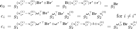
  For the resulting $\mathbf {c} =(\mathbf {c}_{0},c_{1},\dots ,c_{n})$, we have that $\mathbf {c} =\mathbf {E}_{\mathbf {pk}} (\mathbf {u} ^{(b)};\mathbf {r})$ for (independently and uniformly distributed) random coins $\mathbf {r} =(u^{(1)}_{i^*}-u^{(0)}_{i^*})\mathbf {r} ^*+\mathbf {r} '$. Hence, $\mathcal {O}_{\mathbf {enc}}$ returns $\mathbf {c}$.

Finally, $\mathcal {B}$ relays any guess $b'$ from $\mathcal {A}$ as its own output.

Observe that $\mathcal {B}$ perfectly simulates the game from Lemma 1 (with the same challenge bit $b$). We obtain (1).

3.2 The Prime-Order Setting

The Groups. We consider two concrete instantiations of our generic setting. The first is a prime-order setting, in which $\mathbb {G} =\mathbb {G}_1 =\mathbb {G}_2$ has prime order $|\mathbb {G} | =|\mathbb {G}_1 | =|\mathbb {G}_2 |$. In these cases, we assume that $|\mathbb {G} | >2^\lambda$ is public, and hence most syntactic requirements from Sect. 3.1 are trivially met. However, we will additionally need to assume that membership in $\mathbb {G}$ is efficiently decidable. We have numerous candidates for such groups (including, e.g., subgroups of $\mathbb {Z} _p^*$, or elliptic curves). In such groups, plausible assumptions include the Decisional Diffie-Hellman (DDH) assumption, the $k$-Linear ($k$-LIN) assumption [19, 30], or a whole class of assumptions called Matrix-DDH assumptions [10].

Hardness of the GDDH and Factoring Problems. All of the mentioned assumptions imply our GDDH assumption for suitable $\ell _{\mathbf {B}}$ and $\mathbf {B}$. For instance, GDDH with $\ell _{\mathbf {B}} =1$ and uniform $\mathbf {B}$ is nothing but a reformulation of the DDH assumption. More generally, GDDH with uniform $\mathbf {B}$ is actually the so-called $\mathcal {U}_{\ell _{\mathbf {B}}}$-MDDH assumption. In particular, this means that the $k$-LIN assumption implies GDDH with $\ell _{\mathbf {B}} =k$ and uniform $\mathbf {B}$ (see [10]). Additionally, we note that the $\mathbb {G}_2$-factoring assumption we make is trivially satisfied in prime-order settings (since $\mathrm {Adv}^{ fact }_{\mathbb {G}_2,\mathcal {A}} (\lambda )=0$ for all $\mathcal {A}$ if $|\mathbb {G}_2 | =|\mathbb {G} |$ is prime).

Pairing-Friendly Groups. In Sect. 5.4, we also exhibit a building block in the prime-order setting that uses a symmetric pairing $\mathbb {G} \times \mathbb {G} \rightarrow \mathbb {G}_T$ (for a suitable target group $\mathbb {G}_T$). Also for such pairing-friendly groups, we have a variety of candidates in case $\ell _{\mathbf {B}} \ge 2$. (Unfortunately, for $\ell _{\mathbf {B}} =1$, a symmetric pairing can be used to trivially break the GDDH assumption.)

3.3 The DCR Setting

The Public Parameters. The second setting we consider is compatible with the Decisional Composite Residuosity (DCR) assumption [29]. In this case, the global public parameters include an integer $N=PQ$, for distinct safe primes $P,Q$ (i.e., such that $P=2P'+1$ and $Q=2Q'+1$ for prime $P',Q'>2^\lambda$).³ We also assume that $P,Q,P',Q'$ are pairwise different, and that $\gcd (P+Q-1,N)=1$ (the latter of which ensures that $N$ is invertible modulo $\varphi (N)=(P-1)(Q-1)=4P'Q'$).

We implicitly set $\ell _{\mathbf {B}} =1$, and the matrix $\mathbf {B} \in \mathbb {Z} _{|\mathbb {G}_1 | \times |\mathbb {G}_1 |}$ from Sect. 3.1 to be trivial (i.e., the identity matrix). Hence, neither $\ell _{\mathbf {B}}$ nor $g_1 ^{\mathbf {B}}$ will have to be included in the parameters. However, we also include a generator $g_1$ of $\mathbb {G}_1$ in the public parameters, chosen as described below.

The Groups. We now define the groups $\mathbb {G}$, $\mathbb {G}_1$, and $\mathbb {G}_2$. Since $\mathbb {G}$ should only have large prime factors, we should avoid setting $\mathbb {G} =\mathbb {Z} _{N^2}^*$. Instead, we could set $\mathbb {G}_1$ and $\mathbb {G}_2$ to be the subgroups of order $\varphi (N)/4$ and $N$, respectively, and then $\mathbb {G} =\mathbb {G}_1 \cdot \mathbb {G}_2$. However, in this case, membership in $\mathbb {G}$ would not be efficiently decidable in an obvious way. So here, we define our groups in a slightly more complex way, following the approach of signed quadratic residues [11, 13, 20].

Equipped with the notation $|x|_{N}$ and $\left( \frac{x}{N}\right)$ from Sect. 2, we set

$$\begin{aligned} \mathbb {G}_1 \;&=\; \big \{ \; |x^N|_{N^2} \; \big | \; x\in \mathbb {Z} _{N^2}^*,\, \left( \frac{x^N}{N}\right) =1 \; \big \} \;\subseteq \; \mathbb {Z} _{N^2}^* \\ \mathbb {G}_2 \;&=\; \big \{ \; |(1+N)^e|_{N^2} \; \big | \; e\in \mathbb {Z} _N \; \big \} \;\subseteq \; \mathbb {Z} _{N^2}^* \\ \mathbb {G} \;&=\; \big \{ \; |y|_{N^2} \; \big | \; y\in \mathbb {Z} _{N^2}^*,\, \left( \frac{y}{N}\right) =1 \; \big \}. \end{aligned}$$

These sets are groups, when equipped with the group operation $a\cdot b=|a\cdot b|_{N^2}$. Indeed, since $P,Q=3\bmod 4$, we have $\left( \frac{-1}{N}\right) =1$, and thus $\left( \frac{|y_1y_2|_{N^2}}{N}\right) =\left( \frac{y_1y_2}{N}\right) =1$ for $\left( \frac{y_1}{N}\right) =\left( \frac{y_2}{N}\right) =1$. Hence, $\mathbb {G}_1$ and $\mathbb {G}$ are closed under group operation. It is then straightforward to check that $\mathbb {G}_1$, $\mathbb {G}_2$ and $\mathbb {G}$ are groups.

A canonical generator $g_2$ of $\mathbb {G}_2$ is $|1+N|_{N^2}$, and a generator $g_1$ of $\mathbb {G}_1$ (to be included in the public parameters) can be randomly chosen as $|x^N|_{N^2}$ for a uniform $x\in \mathbb {Z} _{N^2}$.

Properties of the Groups. We claim that $|\mathbb {G}_1 | =\varphi (N)/4$. Indeed, we have that

$$\begin{aligned} \big |\big \{ \; |x^N|_{N} \; \big | \; x\in \mathbb {Z} _{N^2}^* \; \big \}\big | \;=\; \big |\big \{ \; |x^N|_{N^2} \; \big | \; x\in \mathbb {Z} _{N^2}^* \; \big \}\big | \;=\; \varphi (N)/2. \end{aligned}$$

In other words, $|x^N|_{N}$ uniquely determines $|x^N|_{N^2}$. Furthermore, since $N$ is invertible modulo $\varphi (N)$, the map $f:\mathbb {Z} _{N^2}^*\rightarrow \mathbb {Z} _N^*$ with $f(x)=x^N\bmod N$ is surjective. Hence, the set of all $|x^N|_{N}$ with $\left( \frac{x^N}{N}\right) =1$ has cardinality $\varphi (N)/4$ (cf. [20, Lemma 1]). Using that $|x^N|_{N}$ fixes $|x^N|_{N^2}$, we obtain $|\mathbb {G}_1 | =\varphi (N)/4$. Moreover, for $e\in \mathbb {Z} _N$, we can write $|(1+N)^e|_{N^2}=|1+eN|_{N^2}=e/|e|+|e|_{N}N$, and thus $|\mathbb {G}_2 | =N$. Finally, we have $\mathbb {G} =\mathbb {G}_1 \cdot \mathbb {G}_2$, since every $|y|_{N^2}\in \mathbb {G}$ can be written as $|y|_{N^2}=|x^N(1+N)^e|_{N^2}$ with $\left( \frac{x^N}{N}\right) =1$. Hence, since $|\mathbb {G}_1 | =\varphi (N)/4=P'Q'$ and $|\mathbb {G}_2 | =N=PQ$ are coprime, $|\mathbb {G} | =|\mathbb {G}_1 | \cdot |\mathbb {G}_2 | =N\cdot \varphi (N)/4$ is square-free.

We also note that the discrete logarithm problem is easy in $\mathbb {G}_2$. Indeed, for $g_2 ^{u}\in \mathbb {G}_2$, we have

A simple case distinction thus allows to compute $[e]_{N}$.

Membership Testing and Sampling Exponents. It is left to note that membership in $\mathbb {G}$ can be efficiently decided (by checking that $y\in \mathbb {Z} _{N^2}$ is invertible, lies between $-N^2/2$ and $N^2/2$, and satisfies $\left( \frac{y}{N}\right) =1$). However, since $|\mathbb {G}_1 |$ will not be public, exponents $s\in \mathbb {Z} _{|\mathbb {G}_1 |}$ can only be sampled approximatively, e.g., by uniformly sampling $s\in \mathbb {Z} _{\lfloor N/4\rfloor }$. This incurs a statistical defect of $\mathbf {O} (1/2^\lambda )$ upon each such sampling. In the following, we will silently ignore these statistical defects (and assume that there is an algorithm that uniformly samples $s\in \mathbb {Z} _{\varphi (N)}$) in our generic constructions for simplicity and ease of presentation. However, we note that the concrete bound (8) also holds for such an approximative sampling in the DCR setting.

Hardness of the GDDH and Factoring Problems. We claim that in the setting described above, the Decisional Composite Residuosity (DCR) assumption [29] implies the GDDH assumption. This connection has already been established in [15, Theorem 2] for a slight variant of the groups $\mathbb {G}$, $\mathbb {G}_1$, $\mathbb {G}_2$ above. (In their setting, $\mathbb {G}_1$ consists of elements $x^N\in \mathbb {Z} _{N^2}$ with $\left( \frac{x^N}{N}\right) =1$, instead of elements $|x^N|_{N^2}$ with $\left( \frac{x^N}{N}\right) =1$.) In fact, their proof applies also to our setting, and we obtain that the DCR assumption implies the GDDH assumption with $\ell =1$ and trivial $\mathbf {B} =1$ in $\mathbb {G}$ (as in Definition 3).

Furthermore, we note that the DCR assumption also implies the $\mathbb {G}_2$-factoring assumption (Definition 4). We sketch how any $\mathbb {G}_2$-factoring adversary $\mathcal {A}$ can be transformed into a DCR adversary $\mathcal {B}$. First, $\mathcal {B}$ runs $\mathcal {A}$, and obtains elements $g_2 ^{u_1},\dots ,g_2 ^{u_q}$. Then, $\mathcal {B}$ uses that the discrete logarithm problem is easy in $\mathbb {G}_2$, and retrieves the corresponding $u_1,\dots ,u_q\in \mathbb {Z} _{|\mathbb {G}_2 |}$. Now if $\gcd (|\mathbb {G}_2 |,u_i)\notin \{1,|\mathbb {G}_2 | \}$ for some $u_i$, then $\gcd (N,u_i)\in \{P,Q\}$ directly allows to factor $N$. Hence, if $\mathcal {A}$ succeeds, then $\mathcal {B}$ can factor $N$, and solve its own DCR challenge (e.g., by computing the order of its input).

4 Tightly Secure Building Blocks

In this section, we describe two building blocks for our main KEM construction. The first, tightly secure one-time signature schemes, is fairly standard, but requires a new instantiation in the DCR setting to achieve tight security. The second is, key extractors, is new, but similar building blocks have been used at least in the prime-order setting implicitly in previous works on tight security (e.g., [12]).

4.1 One-Time Signature Schemes

Definition 6

(Digital signature scheme). A digital signature scheme $\mathbf {OTS} =(\mathbf {SGen},\mathbf {SSig},\mathbf {SVer})$ consists of the following PPT algorithms:

• $\mathbf {SGen} (1^\lambda )$ outputs a keypair $( ovk , osk )$. We call $ovk$ and $osk$ the verification, resp. signing key.

• $\mathbf {SSig} ( osk ,M)$, for a message $M \in \{0,1\}^*$, outputs a signature $\sigma$.

• $\mathbf {SVer} ( ovk ,M,\sigma )$, outputs either $0$ or $1$.

We require correctness in the sense that for all $( ovk , osk )$ that lie in the range of $\mathbf {SGen} (1^\lambda )$, all $M \in \{0,1\}^*$, and all $\sigma$ in the range of $\mathbf {SSig} ( osk ,M)$, we always have $\mathbf {SVer} ( ovk ,M,\sigma )=1$.

We only require one-time security (and call a signature scheme secure in this sense also a one-time signature scheme):

Definition 7

(EUF-MOTCMA security). Let $\mathbf {OTS}$ be a digital signature scheme as in Definition 6, and consider the following game between a challenger $\mathcal {C}$ and an adversary $\mathcal {A}$:

• 1. $\mathcal {C}$ runs $\mathcal {A}$ on input $1^\lambda$, and with (many-time) oracle access to the following oracles:

  • $\mathcal {O}_{\mathbf {gen}} ()$ samples a fresh keypair $( ovk , osk )\leftarrow \mathbf {SGen} ()$, and returns $ovk$.

  • $\mathcal {O}_{\mathbf {sig}} ( ovk ,M)$ first checks if $ovk$ has been generated by $\mathcal {O}_{\mathbf {gen}}$, and returns $\bot$ if not. Next, $\mathcal {O}_{\mathbf {sig}}$ checks if there has been a previous $\mathcal {O}_{\mathbf {sig}} ( ovk ,\cdot )$ query (i.e., an $\mathcal {O}_{\mathbf {sig}}$ query with the same $ovk$), and returns $\bot$ if so. Let $osk$ be the corresponding secret key generated alongside $ovk$. (If $ovk$ has been generated multiple times by $\mathcal {O}_{\mathbf {gen}}$, take the first such $osk$.) $\mathcal {O}_{\mathbf {sig}}$ returns $\sigma \leftarrow \mathbf {SSig} ( osk ,M)$.

• 2. If $\mathcal {A}$ returns $( ovk ^*,M ^*,\sigma ^*)$, such that $\mathbf {SVer} ( ovk ^*,M ^*,\sigma ^*)=1$, and $ovk ^*$ has been returned by $\mathcal {O}_{\mathbf {gen}}$, but $\sigma ^*$ has not been returned by $\mathcal {O}_{\mathbf {sig}} ( ovk ^*,M ^*)$, then $\mathcal {C}$ returns $1$. Otherwise, $\mathcal {C}$ returns $0$.

Let $\mathrm {Adv}^{ ots }_{\mathbf {OTS},\mathcal {A}} (\lambda )$ be the probability that $\mathcal {C}$ finally outputs $1$ in the above game. We say that $\mathbf {OTS}$ is strongly existentially unforgeable under many one-time chosen-message attacks (EUF-MOTCMA secure) iff for every PPT $\mathcal {A}$, the function $\mathrm {Adv}^{ ots }_{\mathbf {OTS},\mathcal {A}} (\lambda )$ is negligible.

We remark, however, that our security notion is “strong”, in the sense that a forger is already successful when he manages to generate a new signature for an already signed message.

A Construction in the Prime-Order Setting. In case $\mathbb {G} =\mathbb {G}_1 =\mathbb {G}_2$ with $|\mathbb {G} |$ prime and public, [18] already give a simple construction of a digital signature scheme that achieves EUF-MOTCMA security under the discrete logarithm assumption. Most importantly for our case, their security reduction is tight (i.e., only loses a constant factor). We refer to their paper for details.

A Construction in the DCR Setting. In the DCR setting (as in Sect. 3.3), there exist simple and efficient EUF-MOTCMA secure signature schemes from the factoring [24] or RSA assumptions [22]. However, these schemes are not known to be tightly secure.

Hence, in the full version [16], we construct a new digital signature scheme whose EUF-MOTCMA security can be tightly reduced to the GDDH assumption in the DCR setting.

4.2 Key Extractors

Intuition. Intuitively, a key extractor derives a pseudorandom key $K$ from a given encryption $\mathbf {c} =\mathbf {E} (0;\mathbf {r})$ of $0$. This $K$ can be derived either publicly, using a public extraction key $xpk$ and the witness $\mathbf {r}$, or secretly, using a secret extraction key $xsk$ and only the ciphertext $\mathbf {c}$. We desire security in the sense keys derived secretly (i.e., using $xsk$) from random ciphertexts $\mathbf {c} =\mathbf {E} (R;\mathbf {r})$ for random $R$ cannot be distinguished from truly random bitstrings $K$. This should hold even for many such challenges, and in the face of oracle access to $xsk$ on “consistent” ciphertexts $\mathbf {c} =\mathbf {E} (0;\mathbf {r})$.

In this sense, key extractors give a computational form of the soundness guarantee provided by universal hash proof systems. We also note that a similar tool has been implicitly used in [12] for a similar purpose in the prime-order setting. Hence, we abstract and generalize their construction in a straightforward way.

Definition. In the following, fix a function $\ell _{\mathrm {ext}} =\ell _{\mathrm {ext}} (\lambda )$. In the following definition, we will choose the value $R$ encrypted in random ciphertexts uniformly from $\mathbb {Z} _{2^{\ell _{\mathrm {ext}}}}$. Our generic construction of key extractors works for any $\ell _{\mathrm {ext}} \ge 3\lambda$ (and $|\mathbb {G}_2 | \ge 2^{3\lambda }$).

Definition 8

(Key extractor). A key extractor $\mathbf {EXT} =(\mathbf {ExtGen},\mathbf {Ext}_{\mathrm {pub}},\mathbf {Ext}_{\mathrm {priv}})$ for $\mathbb {G}$ consists of the following PPT algorithms

• $\mathbf {ExtGen} (1^\lambda , epk )$, on input a public encryption key $epk =g_1 ^{\varvec{\omega } ^\top \mathbf {B}}\in \mathbb {G}_1 ^{\ell _{\mathbf {B}}}$ for $(\mathbf {E},\mathbf {D})$ (as in Sect. 3.1), outputs a keypair $( xpk , xsk )$. We call $xpk$ the public and $xsk$ the private extraction key.

• $\mathbf {Ext}_{\mathrm {pub}} ( xpk ,\mathbf {c},\mathbf {r})$, for $\mathbf {c} =\mathbf {E}_{ epk } (0;\mathbf {r})$, outputs a key $K \in \{0,1\}^\lambda$.

• $\mathbf {Ext}_{\mathrm {priv}} ( xsk ,\mathbf {c})$ also outputs a session key $K \in \{0,1\}^\lambda$.

We require the following:

Correctness. :

For all $epk =g_1 ^{\varvec{\omega } ^\top \mathbf {B}}$, all keypairs $( xpk , xsk )$ that lie in the range of $\mathbf {ExtGen} (1^\lambda , epk )$, all $\mathbf {r} \in \mathbb {Z} _{|\mathbb {G}_1 |}^{\ell _{\mathbf {B}}}$, and all $\mathbf {c} =\mathbf {E}_{ epk } (0;\mathbf {r})$, we always have $\mathbf {Ext}_{\mathrm {pub}} ( xpk ,\mathbf {c},\mathbf {r})=\mathbf {Ext}_{\mathrm {priv}} ( xsk ,\mathbf {c})$.

Indistinguishability. :

Consider the following game between a challenger $\mathcal {C}$ and an adversary $\mathcal {A}$:

• 1. $\mathcal {C}$ uniformly samples $\varvec{\omega } \in \mathbb {Z} _{|\mathbb {G}_1 |}^{\ell _{\mathbf {B}}}$ and sets $( epk , esk )=(g_1 ^{\varvec{\omega } ^\top \mathbf {B}},\varvec{\omega })$. Then, $\mathcal {C}$ generates an $\mathbf {EXT}$ keypair $( xpk , xsk )\leftarrow \mathbf {ExtGen} (1^\lambda , epk )$, and finally samples $b\in \{0,1\}$.

• 2. $\mathcal {A}$ is run on input $(1^\lambda , epk , xpk )$, with (many-time) access to oracles $\mathcal {O}_{\mathbf {cha}}$ and $\mathcal {O}_{\mathbf {ext}}$ that operate as follows:

  • $\mathcal {O}_{\mathbf {cha}} ()$ uniformly chooses a fresh $R\in \mathbb {Z} _{2^{\ell _{\mathrm {ext}}}}$, computes $\mathbf {c} \leftarrow \mathbf {E}_{ epk } (R)$ and $K_{0} =\mathbf {Ext}_{\mathrm {priv}} ( xsk ,\mathbf {c})$, and uniformly chooses $K_{1} \in \{0,1\}^\lambda$. Finally, $\mathcal {O}_{\mathbf {cha}}$ returns $(\mathbf {c},K_{b})$.

  • $\mathcal {O}_{\mathbf {ext}} (\mathbf {c})$ first checks if $\mathbf {D}_{ esk } (\mathbf {c})=g_2 ^{0}$. If not, then we say that $\mathcal {A}$ fails, and $\mathcal {C}$ terminates with output $0$ immediately. Otherwise, $\mathcal {O}_{\mathbf {ext}}$ computes and returns $K =\mathbf {Ext}_{\mathrm {priv}} ( xsk ,\mathbf {c})$.

  • Finally, $\mathcal {A}$ outputs a bit $b'$, and $\mathcal {C}$ outputs $1$ iff $b=b'$ (and $0$ otherwise).

Let $\mathrm {Adv}^{ ext }_{\mathbf {EXT},\mathcal {A}} (\lambda )=\Pr \left[ {\mathcal {C} \text { outputs }1}\right] -1/2$. We require that for all PPT $\mathcal {A}$, $\mathrm {Adv}^{ snd }_{\mathbf {PS},\mathcal {A}} (\lambda )\le \varepsilon$ for a negligible function $\varepsilon =\varepsilon (\lambda )$.

A Generic Construction. For our GDDH-based key extractor, we assume that a function $h$ chosen from a family of universal hash functions $\mathbf {UHF}_{\lambda }$ is made public in the global public parameters $\mathrm {pp}$. Then, our extractor $\mathbf {EXT}^{\mathrm {gddh}} =(\mathbf {ExtGen}^{\mathrm {gddh}},\mathbf {Ext}_{\mathrm {pub}}^{\mathrm {gddh}},\mathbf {Ext}_{\mathrm {priv}}^{\mathrm {gddh}})$ is defined as follows:

• , for , uniformly samples and , and computes . The output of is and .

• , for $xpk$ as above and , outputs .

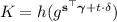• , for , outputs .

Given and a ciphertext , we have

$$\begin{aligned} g_1 ^{\mathbf {w} ^\top \mathbf {r}}=g_1 ^{\mathbf {s} ^\top \mathbf {B} \mathbf {r} +t\cdot \varvec{\omega } ^\top \mathbf {B} \mathbf {r}}=g ^{\mathbf {s} ^\top \varvec{\gamma } +t\cdot \delta }, \end{aligned}$$

and correctness follows. Indistinguishability follows from the following lemma:

Lemma 2

For $\ell _{\mathrm {ext}} \ge 3\lambda$ and $|\mathbb {G}_2 | \ge 2^{3\lambda }$, $\mathbf {EXT}^{\mathrm {gddh}}$ above satisfies the indistinguishability property of Definition 8, assuming GDDH in $\mathbb {G}$. Specifically, for every adversary $\mathcal {A}$ that makes at most $q$ oracle queries, there is an adversary $\mathcal {B}$ (with roughly the same complexity as the indistinguishability experiment with $\mathbf {EXT}^{\mathrm {gddh}}$ and $\mathcal {A}$), such that

$$\begin{aligned} \mathrm {Adv}^{ ext }_{\mathbf {EXT}^{\mathrm {gddh}},\mathcal {A}} (\lambda ) \;\le \; \mathrm {Adv}^{ gddh }_{\mathbb {G},\mathcal {B}} (\lambda ) + q/2^\lambda . \end{aligned}$$

(2)

Due to lack of space, we outsource a proof of Lemma 2 to the full version [16].

Summing up, we obtain

Theorem 1

Under the GDDH assumption, and for $\ell _{\mathrm {ext}} \ge 3\lambda$ and $|\mathbb {G}_2 | \ge 2^{3\lambda }$, $\mathbf {EXT}^{\mathrm {gddh}}$ is a key extractor in the sense of Definition 8.

5 Benign Proof Systems

Intuition. Benign proof systems are the central technical tool in our KEM construction. Intuitively, a benign proof system for some language $\mathcal {L}$ is a non-interactive designated-verifier zero-knowledge proof system with strong soundness guarantees. Concretely, the system guarantees soundness even if simulated proofs for potentially false statements $x\notin \mathcal {L}$ are known. However, we do not quite require “simulation-soundness”, in the sense that this should hold for simulated proofs for arbitrary false statements. (We note that simulation-sound proof systems are extremely useful in the context of tight security proofs, but they are also very hard to construct.)

Instead, we only require that no adversary can forge proofs for statements $x\notin \mathcal {L}$ that are “more false” than any statement for which a simulated proof is known. A little more specifically, we require that even if simulated proofs for statements $x\in \mathcal {L} '\supseteq \mathcal {L}$ are known, an adversary cannot forge a proof for some $x\notin \mathcal {L} '$. The main benefit over existing soundness notions is that $\mathcal {L} '$ does not even have to be known during the construction of the scheme. (For instance, our first proof system provides a “graceful soundness degradation”, in the sense that it is sound in this sense for arbitrary linear languages $\mathcal {L} '\supseteq \mathcal {L}$.)

Overview Over Our Constructions. Apart from the abstraction, we also provide generic and setting-specific constructions of benign proof systems. Our generic constructions (for a linear, and a “dynamically parameterized” linear language) can be viewed as abstractions and generalizations of universal hash proof systems. For $\mathcal {L} '=\mathcal {L}$, soundness in the above sense follows immediately from the correctness property of hash proof systems. (Indeed, hash proofs for valid instances $x\in \mathcal {L}$ are unique and completely determined by public information.) For $\mathcal {L} '\supsetneq \mathcal {L}$, we will use additional properties of specific (existing) hash proof systems. In fact, the mentioned “graceful degradation” guarantees have already been used implicitly in the work of [12].

However, we also consider a somewhat nonstandard (and in our application crucial) “OR-language”. Here, we give a prime-order instantiation in pairing-friendly groups (which is directly implied by the universal hash proof systems for disjunctions from [1]), and a new instance in the DCR setting. This DCR instance will be the key to the DCR-based instantiation of our KEM.

5.1 Definition

Definition 9

(Proof system). Let $\mathcal {L} =\{\mathcal {L} _{ pars }\}$ be a family of languages⁴ with $\mathcal {L} _{ pars }\subseteq \mathcal {X}_{ pars }$, and with efficiently computable witness relation $\mathcal {R}$. A non-interactive designated-verifier proof system (NIDVPS) $\mathbf {PS} =(\mathbf {PGen},\mathbf {PPrv},\mathbf {PVer},\mathbf {PSim})$ for $\mathcal {L}$ consists of the following PPT algorithms:

• $\mathbf {PGen} (1^\lambda , pars )$ outputs a keypair $( ppk , psk )$. We call $ppk$ the public and $psk$ the private key.

• $\mathbf {PPrv} ( ppk ,x,w)$, for $x\in \mathcal {L}$ and $\mathcal {R} (x,w)=1$, outputs a proof $\pi$.

• $\mathbf {PVer} ( psk ,x,\pi )$, for $x\in \mathcal {X}$ and a proof $\pi$, outputs a verdict $b\in \{0,1\}$.

• $\mathbf {PSim} ( psk ,x)$, for $x\in \mathcal {L}$, outputs a proof $\pi$.

We require correctness in the following sense:

• Completeness. For all $pars$, all $( ppk , psk )$ in the range of $\mathbf {PGen} (1^\lambda , pars )$, all $x\in \mathcal {L}$, and all $w$ with $\mathcal {R} ( pars ,x,w)=1$, we always have $\mathbf {PVer} ( psk , x,\mathbf {PPrv} ( ppk ,x,w))=1$.

All relevant security properties of a NIDVPS are condensed in the following definition.

Definition 10

(Benign proof system). Let $\mathbf {PS}$ be an NIDVPS for $\mathcal {L}$ as in Difinition 9, and let , , and be families of languages. We say that $\mathbf {PS}$ is -benign if the following properties hold:

• (Perfect) zero-knowledge. For all $pars$, all $( ppk , psk )$ that lie in the range of $\mathbf {PGen} (1^\lambda , pars )$, and all $x\in \mathcal {L}$ and $w$ with $\mathcal {R} ( pars ,x,w)=1$, we have the following equivalence of distributions:

  $$\begin{aligned} \mathbf {PPrv} ( ppk ,x,w)\quad \equiv \quad \mathbf {PSim} ( psk ,x). \end{aligned}$$

• (Statistical) $(\mathcal {L}^{\mathrm {sim}},\mathcal {L}^{\mathrm {ver}},\mathcal {L}^{\mathrm {snd}})$ -soundness. Consider the following game played between a challenger $\mathcal {C}$ and an adversary $\mathcal {A}$:

• 1. $\mathcal {A}$ is run on input $1^\lambda$, and chooses $pars$.

• 2. $\mathcal {C}$ generates $( ppk , psk )\leftarrow \mathbf {PGen} (1^\lambda , pars )$.

• 3. $\mathcal {A}$ is run again on input $(1^\lambda , ppk )$, and with (many-time) access to oracles $\mathcal {O}_{\mathbf {sim}}$ and $\mathcal {O}_{\mathbf {ver}}$ that operate as follows:

  • $\mathcal {O}_{\mathbf {sim}} (x)$ checks if $x\in \mathcal {L}^{\mathrm {sim}}_{ pars }$, and if yes, returns $\mathbf {PSim} ( psk ,x)$. Otherwise, $\mathcal {O}_{\mathbf {sim}}$ returns $\bot$.

  • $\mathcal {O}_{\mathbf {ver}} (x,\pi )$ checks if $x\in \mathcal {L}^{\mathrm {ver}}_{ pars }$, and, if so, returns $\mathbf {PVer} ( psk ,x,\pi )$. Otherwise, $\mathcal {O}_{\mathbf {ver}}$ returns $\bot$.

Finally, $\mathcal {A}$ wins iff it has queried $\mathcal {O}_{\mathbf {ver}}$ with $(x,\pi )$ such that $x\in \mathcal {X}_{ pars } \setminus \mathcal {L}^{\mathrm {snd}}_{ pars }$ and $\mathbf {PVer} ( psk ,x,\pi )=1$. Let $\mathrm {Adv}^{ snd }_{\mathbf {PS},\mathcal {A}} (\lambda )$ the probability that $\mathcal {A}$ wins. We require that for all (not necessarily computationally bounded) $\mathcal {A}$ that only make a polynomial number of oracle queries, $\mathrm {Adv}^{ snd }_{\mathbf {PS},\mathcal {A}} (\lambda )$ is negligible.

Intuitively, the soundness condition of Definition 10 thus states that no proofs for $\mathcal {X} \setminus \mathcal {L}^{\mathrm {snd}}_{ pars }$-statements can be forged, even when (simulated) proofs for $\mathcal {L}^{\mathrm {sim}}_{ pars }$-statements are available, and proofs for $\mathcal {L}^{\mathrm {ver}}_{ pars }$-statements can be verified.

5.2 The Generic Linear Language

We will be interested in proof systems for “linear languages”, in the sense that instances are vectors of group elements, and the language is closed under vector addition (i.e., componentwise group operation).

In the following, let $D \in \mathbb {N}$ and $\mathbf {pk} =( epk _{1},\dots , epk _{D})=(g_1 ^{\varvec{\omega }_{1} ^\top \mathbf {B}},\dots ,g_1 ^{\varvec{\omega }_{D} ^\top \mathbf {B}})\in (\mathbb {G}_1 ^{\ell _{\mathbf {B}}})^D$. For a concise notation, write $\varvec{\varOmega } =(\varvec{\omega }_{1} ||\dots ||\varvec{\omega }_{D})\in \mathbb {Z} _{|\mathbb {G}_1 |}^{\ell _{\mathbf {B}} \times D}$. Also, fix a $\mathbb {Z} _{|\mathbb {G}_2 |}$-module

$$\begin{aligned} \mathfrak {U} \;=\; \{\mathbf {M} \mathbf {x} \mid \mathbf {x} \in \mathbb {Z} _{|\mathbb {G}_2 |}^d \} \;\subseteq \; \mathbb {Z} _{|\mathbb {G}_2 |}^D \end{aligned}$$

(3)

defined by a matrix $\mathbf {M} \in \mathbb {Z} _{|\mathbb {G}_2 |}^{D \times d}$. Our languages are parameterized over $pars _{\mathrm {lin}} =(\mathbf {pk},\mathbf {M})$, although $\mathcal {L}^{\mathrm {lin}}_{\mathbf {pk}}$ only depends on $\mathbf {pk}$, and not on $\mathbf {M}$. Namely, consider

$$\begin{aligned} \begin{aligned} \mathcal {L}^{\mathrm {lin}}_{\mathbf {pk}} \;&=\; \big \{\mathbf {E}_{\mathbf {pk}} (\mathbf {u};\mathbf {r}) \;\mid \; \mathbf {r} \in \mathbb {Z} _{|\mathbb {G}_1 |}^{\ell _{\mathbf {B}}},\;\mathbf {u} =\mathbf {0} \in \mathbb {Z} _{|\mathbb {G}_2 |}^D \big \} \\ \mathcal {L}_{\mathrm {sim},(\mathbf {pk},\mathbf {M})}^{\mathrm {lin}} \;&=\;\mathcal {L}_{\mathrm {ver},(\mathbf {pk},\mathbf {M})}^{\mathrm {lin}} \;=\;\mathcal {L}_{\mathrm {snd},(\mathbf {pk},\mathbf {M})}^{\mathrm {lin}} \\ \;&=\; \big \{\mathbf {E}_{\mathbf {pk}} (\mathbf {u};\mathbf {r}) \;\mid \; \mathbf {r} \in \mathbb {Z} _{|\mathbb {G}_1 |}^{\ell _{\mathbf {B}}},\;\mathbf {u} \in \mathfrak {U} \big \} \\ \mathcal {X}^{\mathrm {lin}} \;&=\; \mathbb {G} ^{\ell _{\mathbf {B}} +D}, \end{aligned} \end{aligned}$$

(4)

and set $\mathcal {L}^{\mathrm {lin}} =\{\mathcal {L}^{\mathrm {lin}}_{\mathbf {pk}} \}$ and $\mathcal {L}_{\mathrm {sim}}^{\mathrm {lin}} =\mathcal {L}_{\mathrm {ver}}^{\mathrm {lin}} =\mathcal {L}_{\mathrm {snd}}^{\mathrm {lin}} =\{\mathcal {L}_{\mathrm {sim},(\mathbf {pk},\mathbf {M})}^{\mathrm {lin}} \}$. A witness for $x\in \mathcal {L}^{\mathrm {lin}}_{\mathbf {pk}}$ is $\mathbf {r}$.

In the full version [16], we present a simple GDDH-based construction (based upon hash proof systems) of an $(\mathcal {L}_{\mathrm {sim}}^{\mathrm {lin}},\mathcal {L}_{\mathrm {ver}}^{\mathrm {lin}},\mathcal {L}_{\mathrm {snd}}^{\mathrm {lin}})$-benign proof system for $\mathcal {L}^{\mathrm {lin}}$.

5.3 A Dynamically Parameterized Linear Language

In our scheme, we will also use a slight variant of the generic linear language above. Specifically, we will consider a simple “dynamically parameterized” linear language, where one parameter (i.e., coefficient) is determined by the language instance. For a formal description, let $pars _{\mathrm {hash}} =\mathbf {pk} =( epk _{1}, epk _{2})\in (\mathbb {G}_1 ^{\ell _{\mathbf {B}}})^2$, and

$$\begin{aligned} \begin{aligned} \mathcal {L}^{\mathrm {hash}}_{\mathbf {pk}} \;&=\; \big \{ \big (\mathbf {E}_{\mathbf {pk}} (\mathbf {u};\mathbf {r}),\;\tau \big ) \;\mid \; \mathbf {u} =\mathbf {0} \in \mathbb {Z} _{|\mathbb {G}_2 |}^2 \big \} \\ \mathcal {L}_{\mathrm {sim},\mathbf {pk} }^{\mathrm {hash}} \;&=\;\mathcal {L}_{\mathrm {ver},\mathbf {pk} }^{\mathrm {hash}} \;=\;\mathcal {L}_{\mathrm {snd},\mathbf {pk} }^{\mathrm {hash}} \\ \;&=\; \big \{ \big (\mathbf {E}_{\mathbf {pk}} (\mathbf {u};\mathbf {r}),\;\tau \big ) \;\mid \; \mathbf {u} =(u_1,u_2)^\top \in \mathbb {Z} _{|\mathbb {G}_2 |}^2,\;u_2=\tau u_1 \big \} \\ \mathcal {X}^{\mathrm {hash}}_{\mathbf {pk}} \;&=\; \big \{ \big (\mathbf {E}_{\mathbf {pk}} (\mathbf {u};\mathbf {r}),\;\tau \big ) \;\mid \; \mathbf {u} \in \mathbb {Z} _{|\mathbb {G}_2 |}^2 \big \}, \end{aligned} \end{aligned}$$

(5)

where $\mathbf {r}$ and $\tau$ always range over $\mathbb {Z} _{|\mathbb {G}_1 |}^{\ell _{\mathbf {B}}}$ and $\mathbb {Z} _{|\mathbb {G}_2 |}$, respectively. A witness for $x\in \mathcal {L}^{\mathrm {hash}}$ is $\mathbf {r}$. The families $\mathcal {L}^{\mathrm {hash}}$, $\mathcal {L}_{\mathrm {sim}}^{\mathrm {hash}}$, $\mathcal {L}_{\mathrm {ver}}^{\mathrm {hash}}$, and $\mathcal {X}^{\mathrm {hash}}$ are defined in the obvious way.

In the full version [16], we present a simple GDDH-based construction (based upon hash proof systems) of an $(\mathcal {L}_{\mathrm {sim}}^{\mathrm {hash}},\mathcal {L}_{\mathrm {ver}}^{\mathrm {hash}},\mathcal {L}_{\mathrm {snd}}^{\mathrm {hash}})$-benign proof system for $\mathcal {L}^{\mathrm {hash}}$.

5.4 The Generic OR-Language

We will also be interested in the following family $\mathcal {L}^\vee$, together with its “simulation”, “verification” and “soundness” counterparts $\mathcal {L}_{\mathrm {sim}}^{\vee }$, $\mathcal {L}_{\mathrm {ver}}^{\vee }$ and $\mathcal {L}_{\mathrm {snd}}^{\vee }$. Here, the actual languages in $\mathcal {L}^\vee$ are linear like those in $\mathcal {L}^{\mathrm {lin}}$. However, soundness also holds when $\mathcal {L}_{\mathrm {sim}}^{\vee }$-instances are simulated, and those instances have an “OR flavor”.

The language parameters are $pars _{\vee } =(\mathbf {pk},\ell _\vee )$ for $\mathbf {pk} =( epk _{1}, epk _{2})\in (\mathbb {G}_1 ^{\ell _{\mathbf {B}}})^2$, and a function $\ell _\vee =\ell _\vee (\lambda )$. The families $\mathcal {L}^\vee$, $\mathcal {L}_{\mathrm {sim}}^{\vee }$, $\mathcal {L}_{\mathrm {ver}}^{\vee }$, $\mathcal {L}_{\mathrm {snd}}^{\vee }$, and $\mathcal {X}^\vee$ are comprised of the following languages, where we consider all $\mathbf {r} \in \mathbb {Z} _{|\mathbb {G}_1 |}^{\ell _{\mathbf {B}}}$, and $\mathbf {u} =(u_1,u_2)\in (\mathbb {Z} _{|\mathbb {G}_2 |}^*\cup \{0\})^2$:

$$\begin{aligned} \mathcal {L}^\vee _{\mathbf {pk}} =\mathcal {L}_{\mathrm {ver},\mathbf {pk} }^{\vee } \;&=\; \big \{\mathbf {E}_{\mathbf {pk}} (\mathbf {u};\mathbf {r}) \;\mid \; u_1=0 \big \} \\ \mathcal {L}_{\mathrm {sim},(\mathbf {pk},\ell _\vee )}^{\vee } \;&=\; \big \{\mathbf {E}_{\mathbf {pk}} (\mathbf {u};\mathbf {r}) \;\mid \; u_1=0\;\vee \;(|u_1|<2^{\ell _\vee }\,\wedge \,u_2=0)\big \} \\ \mathcal {L}_{\mathrm {snd},\mathbf {pk} }^{\vee } \;&=\; \big \{\mathbf {E}_{\mathbf {pk}} (\mathbf {u};\mathbf {r}) \;\mid \; u_1=0\vee u_2=0\big \} \\ \mathcal {X}^\vee _{\mathbf {pk}} \;&=\; \big \{\mathbf {E}_{\mathbf {pk}} (\mathbf {u};\mathbf {r}) \big \}. \end{aligned}$$

Here, the value $|u_1|$ (in the definition of $\mathcal {L}_{\mathrm {sim},(\mathbf {pk},\ell _\vee )}^{\vee }$ is to be understood simply as the absolute value for signed $\mathbb {Z} _{|\mathbb {G}_2 |}$-values in the prime-order setting, and as $|u_1|=|u_1|_{N}$ in the DCR setting. Observe that $\mathcal {L}^\vee _{\mathbf {pk}} \subseteq \mathcal {L}_{\mathrm {sim},(\mathbf {pk},\ell _\vee )}^{\vee } \subseteq \mathcal {L}_{\mathrm {snd},\mathbf {pk} }^{\vee } \subseteq \mathcal {X}^\vee _{\mathbf {pk}}$. A valid witness for $x\in \mathcal {L}^\vee$ is $\mathbf {r}$.

A Construction in Pairing-Friendly Groups. Now assume that $\mathbb {G} =\mathbb {G}_1 =\mathbb {G}_2$ is a prime-order group equipped with a symmetric pairing. Then, a benign proof system for $\mathcal {L}^\vee$ can be constructed from the universal hash proof systems for disjunctions from [1]. Specifically, [1] construct universal hash proof systems for languages of the form $\mathcal {L} =\{(x_1,x_2)\mid x_1\in \mathcal {L} _{1}\vee x_2\in \mathcal {L} _2\}$, where $\mathcal {L} _i\subseteq \mathbb {G} ^\ell$ are linear languages (i.e., vector spaces over $\mathbb {Z} _{|\mathbb {G} |}$). In our case, given $\mathbf {pk} =( epk _{1}, epk _{2})$, we can thus set

$$\begin{aligned} \begin{aligned} \mathcal {L} _{1} \;&=\; \big \{\mathbf {E}_{ epk _{1}} (0;\mathbf {r}) \big \} \\ \mathcal {L} _{2} \;&=\; \big \{\mathbf {E}_{ epk _{2}} (0;\mathbf {r}) \big \} \\ \mathcal {L} \;&=\; \big \{x=(\mathbf {c}_{0},c_{1},c_{2}) \mid (\mathbf {c}_{0},c_{1})\in \mathcal {L} _{1} \vee (\mathbf {c}_{0},c_{2})\in \mathcal {L} _{2} \big \}. \end{aligned} \end{aligned}$$

(6)

Invoking [1] with these languages yields a NIDVPS $\mathbf {PS}_{\mathbf {pair}}^\vee$ that achieves:

Theorem 2

$\mathbf {PS}_{\mathbf {pair}}^\vee$ is an $(\mathcal {L}_{\mathrm {sim}}^{\vee },\mathcal {L}_{\mathrm {ver}}^{\vee },\mathcal {L}_{\mathrm {snd}}^{\vee })$-benign NIDVPS for $\mathcal {L}^\vee$.

A Construction in the DCR Setting. In the following, we assume an $N=PQ$, and groups $\mathbb {G}$, $\mathbb {G}_1$, $\mathbb {G}_2$ as in Sect. 3.3. In particular, we have $\ell _{\mathbf {B}} =1$, and $\mathbf {B}$ is the trivial (identity) matrix. Furthermore, fix an $\ell _\vee =\ell _\vee (\lambda )$. We additionally assume that $P,Q>2^{\ell _\vee +4\lambda }$. Recall that $g_1, epk _{1}, epk _{2} \in \mathbb {G}_1$ are of order $|\mathbb {G}_1 | =\varphi (N)/4$, and that $g_2 \in \mathbb {G}_2$ is of order $|\mathbb {G}_2 | =N$.

Our $(\mathcal {L}_{\mathrm {sim}}^{\vee },\mathcal {L}_{\mathrm {ver}}^{\vee },\mathcal {L}_{\mathrm {snd}}^{\vee })$-benign proof system $\mathbf {PS}_{\mathbf {DCR}}^\vee$ for $\mathcal {L}^\vee$ is given by the following algorithms:

• $\mathbf {PGen}^{\vee } (1^\lambda )$ uniformly chooses $s_1,s_2\in \mathbb {Z} _{\lfloor N^2/4\rfloor }$ and then outputs $ppk _{\vee } =( epk _{1} ^{s_1}, epk _{1} ^{s_2})$ and $psk _{\vee } =(s_1,s_2)$.

• $\mathbf {PPrv}^{\vee } ( ppk _{\vee },x,r)$ (with $ppk _{\vee } =( epk _{1} ^{s_1}, epk _{1} ^{s_2})$, and $x=(c_{0},c_{1},c_{2})=(g_1 ^r, epk _{1} ^r, epk _{2} ^rg_2 ^{u_2})$) uniformly chooses $t_1,t_2\in \mathbb {Z} _N$, and outputs

  $$\begin{aligned} \pi _{\vee } \;=\; (\pi _{0},\pi _{1},\pi _{2}) \;=\; \big (c_{2} ^{t_1+N\cdot t_2},\;( epk _{1} ^{s_1})^r\cdot g_2 ^{t_1},\;( epk _{1} ^{s_2})^r\cdot g_2 ^{t_2}\big ). \end{aligned}$$

• $\mathbf {PVer}^{\vee } ( psk _{\vee },x,\pi _{\vee })$ (for $psk =(s_1,s_2)$, $x=(c_{0},c_{1},c_{2})$, and $\pi _{\vee } =(\pi _{0},\pi _{1},\pi _{2})$) first checks that $\pi _{1}/c_{1} ^{s_1}=g_2 ^{t_1}$ and $\pi _{2}/c_{1} ^{s_2}=g_2 ^{t_2}$ for some $t_1,t_2\in \mathbb {Z} _N$ (and outputs $0$ if not). $\mathbf {PVer}$ then computes⁵ these $t_1,t_2$, and outputs $1$ iff $\pi _{0} =c_{2} ^{t_1+N\cdot t_2}$.

• $\mathbf {PSim}^{\vee } ( psk _{\vee },x)$ (for $psk =(s_1,s_2)$ and $x=(c_{0},c_{1},c_{2})$) uniformly picks $t_1,t_2\in \mathbb {Z} _{N^2}$ and outputs

  $$\begin{aligned} \pi _{\vee } \;=\; (\pi _{0},\pi _{1},\pi _{2}) \;=\; \big (c_{2} ^{t_1+N\cdot t_2},\;c_{1} ^{s_1}\cdot g_2 ^{t_1},\;c_{1} ^{s_2}\cdot g_2 ^{t_2}\big ). \end{aligned}$$

The completeness and zero-knowledge properties of $\mathbf {PS}_{\mathbf {DCR}}^\vee$ follow directly from the fact that $c_{1} ^{s_i}=( epk _{1} ^r)^{s_i}=( epk _{1} ^{s_i})^r$. To show the soundness of $\mathbf {PS}_{\mathbf {DCR}}^\vee$, we prove a helpful technical lemma:

Lemma 3

Let $s_1,s_2,t_1,t_2$ be distributed as in $\mathbf {PS}_{\mathbf {DCR}}^\vee$, and fix any $u\in \mathbb {Z}$ with $|u|<2^{\ell _\vee }$. Let⁶

$$\begin{aligned} aux \;:=\; ([s_1]_{\varphi (N)/4},\;[s_2]_{\varphi (N)/4}, \;[t_1+N\cdot t_2]_{\varphi (N)/4}, \;[us_1+t_1]_{N},\;[us_2+t_2]_{N}), \end{aligned}$$

and write⁷ $w_1:=[s_1/\alpha ]_{N}$ (with the division performed in $\mathbb {Z} _N$) for $\alpha :=[N]_{\varphi (N)/4}$. Then, for an independently random $R\in \mathbb {Z} _{2^\lambda }$, we have

$$\begin{aligned} \varepsilon \;:=\;\mathbf {SD}\big ({([w_1]_{2^\lambda }, aux )}\,;\,{(R, aux )}\big ) \;\le \;3/2^\lambda . \end{aligned}$$

In other words, $w_1$ (and thus $s_1$) is unpredictable, even given $aux$.

Proof

Without loss of generality, assume $u\ge 0$. (For $u<0$, we can invoke the lemma with $-u$, $-t_1$, and $-t_2$ in place of $u$, $t_1$ and $t_2$.) We proceed in steps, in each step modifying $aux$, and bounding the impact on $\varepsilon$. Specifically, in the following, we will define a number of random variables $aux _{i}$, and abbreviate $\varepsilon _i:=\mathbf {SD}\big ({([w_1]_{2^\lambda }, aux _{i})}\,;\,{(R, aux _{i})}\big )$. As a starting point, consider

$$\begin{aligned} aux _{1} \;:=\; ([t_1+N\cdot t_2]_{\varphi (N)/4},\;[us_1+t_1]_{N},\;[us_2+t_2]_{N}). \end{aligned}$$

Now note that $w_1=[s_1/\alpha ]_{N}$ and the $[us_i+t_i]_{N}$ (for $i\in \{1,2\}$) only depend on $[s_i]_{N}$. However, our uniform choice of $s_i\in \mathbb {Z} _{\lfloor N^2/4\rfloor }$ is statistically $2/2^{\ell _\vee +4\lambda }$-close to a uniform choice of $s_i\in \mathbb {Z} _{N\cdot \varphi (N)/4}$ (in which case $[s_i]_{N}$ and $[s_i]_{\varphi (N)/4}$ are independently and uniformly random). Hence, the $[s_i]_{\varphi (N)/4}$ are essentially independent of $w_1$ and $aux _{1}$, and we obtain $\varepsilon \le \varepsilon _1+4/2^{\ell _\vee +4\lambda }$. Next, consider

$$\begin{aligned} aux _{2} \;:=\; ([t_1]_{\alpha },\;[t_2]^{\alpha },\;[t_1]^{\alpha }+[t_2]_{\alpha }, \;[us_1+t_1]_{N},\;[us_2+t_2]_{N}). \end{aligned}$$

Since $t_1+\alpha \cdot t_2=[t_1]_{\alpha }+\alpha \cdot ([t_1]^{\alpha }+[t_2]_{\alpha })+\alpha ^2\cdot [t_2]^{\alpha }$, we have that $aux _{1}$ is a function of $aux _{2}$, and so $\varepsilon _1\le \varepsilon _2$. Similarly, we can refine the last two components of $aux _{2}$ to obtain

$$\begin{aligned} aux _{3} \;:=\; ([t_1]_{\alpha },\;[t_2]^{\alpha },\;[t_1]^{\alpha }+[t_2]_{\alpha }, \;[us_1+\alpha \cdot [t_1]^{\alpha }]_{N},\;[us_2+[t_2]_{\alpha }]_{N}). \end{aligned}$$

Again, $\varepsilon _2\le \varepsilon _3$ since $aux _{3}$ fully defines $aux _{2}$. Similar to our first step, now $[t_1]_{\alpha }$ and $[t_2]^{\alpha }$ are essentially independent of the remaining parts of $aux$ (up to a statistical defect of at most $2/2^{\ell _\vee +4\lambda }$ for each). Hence, for

$$\begin{aligned} aux _{4} \;:=\; ([t_1]^{\alpha }+[t_2]_{\alpha }, \;[us_1+\alpha \cdot [t_1]^{\alpha }]_{N},\;[us_2+[t_2]_{\alpha }]_{N}), \end{aligned}$$

we get that $\varepsilon _3\le \varepsilon _4+4/2^{\ell _\vee +4\lambda }$. Now let $w_2:=[s_2]_{N}$, and consider

$$\begin{aligned} aux _{5} \;:=\; ([t_1]^{\alpha }+[t_2]_{\alpha },\;uw_1+[t_1]^{\alpha },\;uw_2+[t_2]_{\alpha }). \end{aligned}$$

Since $aux _{4}$ can be computed from $aux _{5}$, we have $\varepsilon _4\le \varepsilon _5$. Next, we release $w_1+w_2$ (over $\mathbb {Z}$):

$$\begin{aligned} aux _{6} \;:=\; ([t_1]^{\alpha }+[t_2]_{\alpha },\;w_1+w_2,\;uw_1+[t_1]^{\alpha }). \end{aligned}$$

Again, $aux _{5}$ can be computed from $aux _{6}$, and hence $\varepsilon _5\le \varepsilon _6$. Since we consider the statistical distance between $[w_1]_{2^\lambda }$ and $R$, we can release (and then drop) $[w_1]^{2^{\lambda }}$. Concretely, consider

$$\begin{aligned} aux _{7} \;&:=\;([t_1]^{\alpha }+[t_2]_{\alpha }, \;[w_1]_{2^\lambda }+w_2,\;u\cdot [w_1]_{2^\lambda }+[t_1]^{\alpha },\;[w_1]^{2^\lambda }), \\ aux _{8} \;&:=\;([t_1]^{\alpha }+[t_2]_{\alpha }, \;[w_1]_{2^\lambda }+w_2,\;u\cdot [w_1]_{2^\lambda }+[t_1]^{\alpha }) \\ aux _{9} \;&:=\;([t_1]^{\alpha }+[t_2]_{\alpha }, \;u\cdot [w_1]_{2^\lambda }+[t_1]^{\alpha }). \end{aligned}$$

Here, $\varepsilon _6\le \varepsilon _7$ since $aux _{6}$ can be computed from $aux _{7}$. Moreover, recall that $N>2^{2\ell _\vee +8\lambda }$ by our choice of $P,Q>2^{\ell _\vee +4\lambda }$. Hence, $\varepsilon _7\le \varepsilon _8+1/2^{2\ell _\vee +7\lambda }$, since $[w_1]_{2^\lambda }$ and $[w_1]^{2^\lambda }$ are independent up to a statistical defect of at most $1/2^{2\ell _\vee +7\lambda }$. Finally, $\varepsilon _8\le \varepsilon _9+1/2^{2\ell _\vee +7\lambda }$, since $w_2$ is uniformly and independently random chosen from $\mathbb {Z} _N$.

Similarly, we can show that $[t_2]_{\alpha }$ blinds $[[t_1]^{\alpha }]_{2^{\ell _\vee +2\lambda }}$:

$$\begin{aligned} aux _{10} \;&:=\;([[t_1]^{\alpha }]_{2^{\ell _\vee +2\lambda }}+[t_2]_{\alpha }, \;u\cdot [w_1]_{2^\lambda }+[[t_1]^{\alpha }]_{2^{\ell _\vee +2\lambda }}, \;[[t_1]^{\alpha }]^{2^{\ell _\vee +2\lambda }}), \\ aux _{11} \;&:=\;([[t_1]^{\alpha }]_{2^{\ell _\vee +2\lambda }}+[t_2]_{\alpha }, \;u\cdot [w_1]_{2^\lambda }+[[t_1]^{\alpha }]_{2^{\ell _\vee +2\lambda }}), \\ aux _{12} \;&:=\;(u\cdot [w_1]_{2^\lambda }+[[t_1]^{\alpha }]_{2^{\ell _\vee +2\lambda }}). \end{aligned}$$

With the same reasoning as in $aux _{7}$-$aux _{9}$ (and using that $\alpha ,N/\alpha >2^{\ell _\vee +4\lambda }/2$ by $P,Q>2^{\ell _\vee +4\lambda }$), we get $\varepsilon _9\le \varepsilon _{10}$, as well as $\varepsilon _{10}\le \varepsilon _{11}+1/2^{2\lambda }$, and $\varepsilon _{11}\le \varepsilon _{12}+1/2^{2\lambda }$. Finally, if we set $aux _{13}:=()$ to be the empty sequence, we get $\varepsilon _{12}\le \varepsilon _{13}+1/2^\lambda +2/2^{\ell _\vee +4\lambda }$, since $[t_1]^{\alpha }$ is $2/2^{\ell _\vee +4\lambda }$-close to uniform over $\mathbb {Z} _{\lceil N/\alpha \rceil }$ (which implies that $[[t_1]^{\alpha }]_{2^{\ell _\vee +2\lambda }}$ blinds $u\cdot [w_1]_{2^\lambda }$). It is left to observe that $\varepsilon _{13}=\mathbf {SD}\big ({[w_1]_{2^\lambda }}\,;\,{R}\big ) \le 1/2^{2\ell _\vee +7\lambda }$, since $w_1\in \mathbb {Z} _N$ is uniformly random. Summing up, we get $\varepsilon \le 1/2^\lambda +2/2^{2\lambda }+10/2^{\ell _\vee +4\lambda }+3/2^{2\ell _\vee +7\lambda }\le 3/2^\lambda$, as desired.

We can now proceed to show the soundness of $\mathbf {PS}_{\mathbf {DCR}}^\vee$:

Lemma 4

$\mathbf {PS}_{\mathbf {DCR}}^\vee$ is statistically $(\mathcal {L}_{\mathrm {sim}}^{\vee },\mathcal {L}_{\mathrm {ver}}^{\vee },\mathcal {L}_{\mathrm {snd}}^{\vee })$-sound in the sense of Definition 10. Concretely, for an adversary $\mathcal {A}$ that makes at most $q=q(\lambda )$ oracle queries in the soundness game from Definition 10,

$$\begin{aligned} \mathrm {Adv}^{ snd }_{\mathbf {PS}_{\mathbf {DCR}}^\vee ,\mathcal {A}} (\lambda )\;\le \;4q/2^\lambda . \end{aligned}$$

(7)

Proof

Fix $\ell _\vee$ and $\mathbf {pk}$, and let $\mathbf {view}_{\mathcal {A}}$ be $\mathcal {A}$ ’s view in a run of the computational soundness game from Definition 10. Specifically, $\mathbf {view}_{\mathcal {A}}$ consists of $\mathcal {A}$ ’s input $ppk _{\vee } =( epk _{1} ^{s_1}, epk _{1} ^{s_2})$, as well as all oracle queries (and the corresponding answers). We first consider to what extent $\mathbf {view}_{\mathcal {A}}$ determines the secret key $psk _{\vee } =(s_1,s_2)$.

• $\mathcal {A}$ ’s input $ppk _{\vee } =( epk _{1} ^{s_1}, epk _{1} ^{s_2})$ only depends on $[s_1]_{\varphi (N)/4}$ and $[s_2]_{\varphi (N)/4}$ (since $epk _{1}$ has order $\varphi (N)/4$).

• Each $\mathcal {O}_{\mathbf {sim}}$ oracle query of $\mathcal {A}$ reveals a value $\pi _{\vee } = (\pi _{0},\pi _{1},\pi _{2}) = (c_{2} ^{t_1+N\cdot t_2}, c_{1} ^{s_1}\cdot g_2 ^{t_1}, c_{1} ^{s_2}\cdot g_2 ^{t_2})$ for $\mathcal {A}$-supplied $c_{1},c_{2}$ and fresh $t_1,t_2$. We may assume that $c_{1} = epk _{1} ^r\cdot g_2 ^{u_1}$ and $c_{2} = epk _{2} ^r\cdot g_2 ^{u_2}$ with $u_1=0$ or $|u_1|_{N}<2^{\ell _\vee }\wedge u_2=0$ (since otherwise, $\mathcal {O}_{\mathbf {sim}}$ rejects the query). Hence, such a query reveals

  $$ (\pi _{0},\pi _{1},\pi _{2}) \;=\; ( epk _{2} ^{r(t_1+N\cdot t_2)}g_2 ^{u_2t_1}, \; epk _{1} ^{rs_1}\cdot g_2 ^{u_1s_1+t_1}, \; epk _{1} ^{rs_2}\cdot g_2 ^{u_1s_2+t_2}), $$

  which only depends on $[s_1]_{\varphi (N)/4}$, $[s_2]_{\varphi (N)/4}$, $[t_1+N\cdot t_2]_{\varphi (N)/4}$, $[u_2t_1]_{N}$, as well as $[u_1s_1+t_1]_{N}$ and $[u_1s_2+t_2]_{N}$. Thus, if $u_1=0$, the query reveals only $[s_1]_{\varphi (N)/4}$ and $[s_2]_{\varphi (N)/4}$ about $(s_1,s_2)$. But if $u_1\ne 0$ (and thus $u_2=0$), we can apply Lemma 3 with $u:=u_1$, where we represent $u_1\in \mathbb {Z} _N$ as an integer between $-N/2$ and $N/2$. This yields that the query leaves $[w_1]_{2^\lambda }$ undetermined, up to a small statistical defect. A hybrid argument over all of $\mathcal {A}$ ’s $\mathcal {O}_{\mathbf {sim}}$ queries shows that the overall statistical defect is bounded by $3q/2^\lambda$.

• An $\mathcal {O}_{\mathbf {ver}}$ query on input $(x,\pi _{\vee })$ yields $\bot$ unless $x\in \mathcal {L}_{\mathrm {ver},(\mathbf {pk},\ell _\vee )}^{\vee } =\mathcal {L}^\vee _{(\mathbf {pk},\ell _\vee )}$. But for $x=(c_{0},c_{1},c_{2})=(g_1 ^r, epk _{1} ^r, epk _{2} ^rg_2 ^{u_2})\in \mathcal {L}^\vee _{(\mathbf {pk},\ell _\vee )}$, we get that $\mathcal {O}_{\mathbf {ver}}$ ’s output only depends on $c_{1} ^{s_i}= epk _{1} ^{rs_i}$, and hence only on $[s_i]_{\varphi (N)/4}$ (for $i=1,2$).

To summarize, $\mathbf {view}_{\mathcal {A}}$ is essentially independent of $[w_1]_{2^\lambda }$, up to a statistical defect of $3q/2^\lambda$.

It remains to prove that any $\mathcal {O}_{\mathbf {ver}}$ query on some $(x,\pi _{\vee })$ with $x\in \mathcal {X}^\vee \setminus \mathcal {L}_{\mathrm {snd},\mathbf {pk} }^{\vee }$ (i.e., an $x$ with $x = (c_{0},c_{1},c_{2}) = (g_1 ^r, epk _{1} ^r\cdot g_2 ^{u_1}, epk _{2} ^r\cdot g_2 ^{u_2})$ for $u_1,u_2\in \mathbb {Z} _N^*$) is invalid in the sense that $\mathbf {PVer} ( psk _{\vee },x,\pi _{\vee })=0$ with high probability. To this end, write

$$\begin{aligned} \pi _{\vee } \;=\; (\pi _{0},\pi _{1},\pi _{2}) \;=\; ( epk _{2} ^{\rho _0}\cdot g_2 ^{\alpha _0}, \; epk _{1} ^{\rho _1}\cdot g_2 ^{\alpha _1}, \; epk _{1} ^{\rho _2}\cdot g_2 ^{\alpha _2}) \end{aligned}$$

for suitable $\rho _0,\rho _1,\rho _2,\alpha _0,\alpha _1,\alpha _2$. Recall that $(x,\pi _{\vee })$ is valid only if for $i=1,2$, we have $\pi _{i}/c_{1} ^{s_i}=g_2 ^{t_i}$ for some $t_i\in \mathbb {Z} _N$, and if $\pi _{0} =c_{2} ^{t_1+N\cdot t_2}$ for those $t_i$. Hence, if $(x,\pi _{\vee })$ is valid, then the following holds for some $t_1,t_2$:

$$\begin{aligned} \rho _0&=[r(t_1+N\cdot t_2)]_{\varphi (N)/4}&\qquad \alpha _0&=[u_2t_1]_{N} \\ \rho _1&=[rs_1]_{\varphi (N)/4}&\qquad \alpha _1&=[u_1s_1+t_1]_{N} \\ \rho _2&=[rs_2]_{\varphi (N)/4}&\qquad \alpha _2&=[u_1s_2+t_2]_{N}. \end{aligned}$$

By assumption, $u_2\in \mathbb {Z} _N^*$, and thus $\alpha _0$ determines $t_1$. Using also $u_1\in \mathbb {Z} _N^*$, hence $\alpha _0$ and $\alpha _1$ determine $[s_1]_{N}$, and thus also $w_1=[s_1/\alpha ]_{N}$. However, as we have argued above, $\mathbf {view}_{\mathcal {A}}$ is essentially independent of $[w_1]_{2^\lambda }$. The probability that $\mathcal {A}$ correctly guesses an independently and uniformly random $[w_1]_{2^\lambda }$ with a single query is exactly $1/2^\lambda$. Since $\mathcal {A}$ makes at most $q$ guesses, the probability for a correct guess is bounded by $q/2^\lambda$. Taking into account the mentioned statistical defect in $\mathbf {view}_{\mathcal {A}}$, we obtain (7).

Taking things together, we obtain

Theorem 3

$\mathbf {PS}_{\mathbf {DCR}}^\vee$ is an $(\mathcal {L}_{\mathrm {sim}}^{\vee },\mathcal {L}_{\mathrm {ver}}^{\vee },\mathcal {L}_{\mathrm {snd}}^{\vee })$-benign NIDVPS for $\mathcal {L}^\vee$.

6 The Key Encapsulation Scheme

In the following, we present our main construction of an IND-MCCA secure key encapsulation (KEM) scheme. (This directly implies a PKE scheme with the same security properties [8].)

6.1 The Construction

Ingredients and Public Parameters. In our construction, we use the following ingredients:

• groups $\mathbb {G}$, $\mathbb {G}_1$, $\mathbb {G}_2$ with $|\mathbb {G}_2 | >2^{3\lambda }$ (see Sect. 3.1 for a description of the generic setting),

• the generalized ElGamal scheme $(\mathbf {E},\mathbf {D})$ implicitly defined through $\mathbb {G}$, $\mathbb {G}_1$, $\mathbb {G}_2$ (Sect. 3.1),

• an EUF-MOTCMA secure one-time signature scheme $\mathbf {OTS} =(\mathbf {SGen},\mathbf {SSig},\mathbf {SVer})$ (Sect. 4.1),

• a key extractor $\mathbf {EXT} =(\mathbf {ExtGen},\mathbf {Ext}_{\mathrm {pub}}, \mathbf {Ext}_{\mathrm {priv}})$ for $\mathbb {G}$ (see Sect. 4.2) with $\ell _{\mathrm {ext}} =3\lambda$,

• an $(\mathcal {L}_{\mathrm {sim}}^{\mathrm {lin}},\mathcal {L}_{\mathrm {ver}}^{\mathrm {lin}},\mathcal {L}_{\mathrm {snd}}^{\mathrm {lin}})$-benign proof system denoted with $\mathbf {PS}^{\mathrm {lin}} =(\mathbf {PGen}^{\mathrm {lin}},\mathbf {PPrv}^{\mathrm {lin}},\mathbf {PVer}^{\mathrm {lin}},\mathbf {PSim}^{\mathrm {lin}})$ for $\mathcal {L}^{\mathrm {lin}}$ (Sect. 5.2),

• an $(\mathcal {L}_{\mathrm {sim}}^{\mathrm {hash}},\mathcal {L}_{\mathrm {ver}}^{\mathrm {hash}},\mathcal {L}_{\mathrm {snd}}^{\mathrm {hash}})$-benign proof system denoted $\mathbf {PS}^{\mathrm {hash}} =(\mathbf {PGen}^{\mathrm {hash}},\mathbf {PPrv}^{\mathrm {hash}},\mathbf {PVer}^{\mathrm {hash}},\mathbf {PSim}^{\mathrm {hash}})$ for $\mathcal {L}^{\mathrm {hash}}$ (Sect. 5.3),

• an $(\mathcal {L}_{\mathrm {sim}}^{\vee },\mathcal {L}_{\mathrm {ver}}^{\vee },\mathcal {L}_{\mathrm {snd}}^{\vee })$-benign proof system denoted $\mathbf {PS}^{\vee } =(\mathbf {PGen}^{\vee },\mathbf {PPrv}^{\vee },\mathbf {PVer}^{\vee },\mathbf {PSim}^{\vee })$ for $\mathcal {L}^\vee$ (Sect. 5.4) with $\ell _\vee =3\lambda$, and

• a collision-resistant hash function generator $\mathbf {CRHF}$ (Sect. 2) with $\ell _{H} =2\lambda$.⁸

We can use the presented generic constructions for $\mathbf {EXT}$, $\mathbf {PS}^{\mathrm {lin}}$, and $\mathbf {PS}^{\mathrm {hash}}$, and, in the prime-order and DCR settings, the presented concrete constructions for $\mathbf {OTS}$ and $\mathbf {PS}^{\vee }$. (We note, however, that the DCR-based proof system $\mathbf {PS}_{\mathbf {DCR}}^\vee$ additionally requires that $|\mathbb {G} |$ has no prime factors smaller than $2^{7\lambda }$.) Specifically, we obtain instantiations both in the prime-order (with symmetric pairing) and DCR settings.

We also assume public parameters $\mathrm {pp}$ that contain whatever public parameters our building blocks require. Specifically, $\mathrm {pp}$ defines groups $\mathbb {G}$, $\mathbb {G}_1$, and $\mathbb {G}_2$ (as described in Sect. 3.1), and contains a hash function $H$ output by $\mathbf {CRHF}$.

The Algorithms. Now our KEM $\mathbf {KEM}$ is defined through the following algorithms:

• $\mathbf {Gen} (1^\lambda )$ first uniformly picks $\varvec{\omega }_{1},\dots ,\varvec{\omega }_{4} \in \mathbb {Z} _{|\mathbb {G}_1 |}^{\ell _{\mathbf {B}}}$, and sets $(\mathbf {pk},\mathbf {sk})=( epk _{i}, esk _{i})_{i=1}^4=(g_1 ^{\varvec{\omega }_{i} ^\top \mathbf {B}},\varvec{\omega }_{i})_{i=1}^4$. Next, $\mathbf {Gen}$ samples

  $$\begin{aligned} ( ppk _{\mathrm {lin}}, psk _{\mathrm {lin}}) \;&\leftarrow \; \mathbf {PGen}^{\mathrm {lin}} (1^\lambda ,\mathbf {pk}) \\ ( ppk _{\mathrm {hash}}, psk _{\mathrm {hash}}) \;&\leftarrow \; \mathbf {PGen}^{\mathrm {hash}} (1^\lambda ,( epk _{1}, epk _{2}/ epk _{3})) \\ {} ( ppk _{\vee ,1}, psk _{\vee ,1}) \;&\leftarrow \; \mathbf {PGen}^{\vee } (1^\lambda ,( epk _{1}, epk _{1})) \\ {} ( ppk _{\vee ,2}, psk _{\vee ,2}) \;&\leftarrow \; \mathbf {PGen}^{\vee } (1^\lambda ,( epk _{4}, epk _{4})) \\ {} ( ppk _{\vee ,3}, psk _{\vee ,3}) \;&\leftarrow \; \mathbf {PGen}^{\vee } (1^\lambda ,( epk _{4}, epk _{1})) \\ {} ( ppk _{\vee ,4}, psk _{\vee ,4}) \;&\leftarrow \; \mathbf {PGen}^{\vee } (1^\lambda ,( epk _{2}/ epk _{3}, epk _{4})) \\ {} ( ppk _{\vee ,5}, psk _{\vee ,5}) \;&\leftarrow \; \mathbf {PGen}^{\vee } (1^\lambda ,( epk _{2}/ epk _{3}, epk _{4})) \\ {} ( ppk _{\vee ,6}, psk _{\vee ,6}) \;&\leftarrow \; \mathbf {PGen}^{\vee } (1^\lambda ,( epk _{2}/ epk _{3}, epk _{1})) \\ ( xpk , xsk ) \;&\leftarrow \; \mathbf {ExtGen} (1^\lambda , epk _{2}), \end{aligned}$$

  sets $\mathbf {ppk} =( ppk _{\mathrm {lin}}, ppk _{\mathrm {hash}}, ppk _{\vee ,1},\dots , ppk _{\vee ,6})$ and $\mathbf {psk} =( psk _{\mathrm {lin}}, psk _{\mathrm {hash}}, psk _{\vee ,1},\dots , psk _{\vee ,6})$, and finally outputs

  $$\begin{aligned} pk \;&=\; (\mathbf {pk},\mathbf {ppk}, xpk )&sk \;&=\; (\mathbf {sk},\mathbf {psk}, xsk ). \end{aligned}$$

• $\mathbf {Enc} ( pk )$ (for $pk$ as above) selects a random $\mathbf {r}$, and computes

  $$\begin{aligned} \mathbf {c} =(\mathbf {c}_{0},c_{1},\dots ,c_{4}) \;&=\; \mathbf {E} (\mathbf {pk},\mathbf {0};\mathbf {r}) \\ ( ovk , osk ) \;&\leftarrow \; \mathbf {SGen} () \\ \tau \;&=\; H ( ovk ) \\ \pi _{\mathrm {lin}} \;&\leftarrow \; \mathbf {PPrv}^{\mathrm {lin}} ( ppk _{\mathrm {lin}},\mathbf {c},\mathbf {r}) \\ \pi _{\mathrm {hash}} \;&\leftarrow \; \mathbf {PPrv}^{\mathrm {hash}} ( ppk _{\mathrm {hash}},((\mathbf {c}_{0},c_{1},c_{2}/c_{3}),\tau ),\mathbf {r}) \\ \pi _{\vee ,1} \;&\leftarrow \; \mathbf {PPrv}^{\vee } ( ppk _{\vee ,1},(\mathbf {c}_{0},c_{1},c_{1}/g_2),\mathbf {r}) \\ \pi _{\vee ,2} \;&\leftarrow \; \mathbf {PPrv}^{\vee } ( ppk _{\vee ,2},(\mathbf {c}_{0},c_{4},c_{4}/g_2),\mathbf {r}) \\ \pi _{\vee ,3} \;&\leftarrow \; \mathbf {PPrv}^{\vee } ( ppk _{\vee ,3},(\mathbf {c}_{0},c_{4},c_{1}/g_2),\mathbf {r}) \\ \pi _{\vee ,4} \;&\leftarrow \; \mathbf {PPrv}^{\vee } ( ppk _{\vee ,4},(\mathbf {c}_{0},c_{2}/c_{3},c_{4}),\mathbf {r}) \\ \pi _{\vee ,5} \;&\leftarrow \; \mathbf {PPrv}^{\vee } ( ppk _{\vee ,5},(\mathbf {c}_{0},c_{2}/c_{3},c_{4}/g_2),\mathbf {r}) \\ \pi _{\vee ,6} \;&\leftarrow \; \mathbf {PPrv}^{\vee } ( ppk _{\vee ,6},(\mathbf {c}_{0},c_{2}/c_{3},c_{1}/g_2),\mathbf {r}) \\ \varvec{\pi }_{} \;&=\; (\pi _{\mathrm {lin}},\pi _{\mathrm {hash}},\pi _{\vee ,1},\dots ,\pi _{\vee ,6}) \\ \sigma \;&\leftarrow \; \mathbf {SSig} ( osk ,(\mathbf {c},\varvec{\pi }_{})) \\ K \;&=\; \mathbf {Ext}_{\mathrm {pub}} ( xpk ,(\mathbf {c}_{0},c_{2}),\mathbf {r}). \end{aligned}$$

  Here, we interpret $\tau =(\tau _1,\dots ,\tau _{2\lambda })\in \{0,1\}^{2\lambda }$ as an integer $\tau =\sum _{i=1}^{2\lambda }2^{i-1}\tau _i\in \{0,\dots ,2^{2\lambda }-1\}$, with $\tau _1$ being interpreted as the least significant bit. The final output of $\mathbf {Enc}$ is $C =(\mathbf {c},\varvec{\pi }_{}, ovk ,\sigma )$ and $K$.

• $\mathbf {Dec} ( sk ,C)$ (for $sk$ and $C$ as above), first verifies $\sigma$ and all proofs in $\varvec{\pi }_{}$ using $ovk$ and $\mathbf {sk}$, and, if all are valid, returns

  $$ K \;=\; \mathbf {Ext}_{\mathrm {priv}} ( xsk ,(\mathbf {c}_{0},c_{2})). $$

Explanation. The proofs in $\varvec{\pi }_{}$ require some explanation. They prove various (seemingly highly redundant) properties of the vector $\mathbf {u} =(u_i)_{i=1}^4\in \mathbb {Z} _{|\mathbb {G}_2 |}^4$ encrypted in $\mathbf {c}$. Some of these properties will be violated in different steps of our security analysis already by the security game, and we will then rely on the remaining properties. For instance, $\pi _{\mathrm {lin}}$ always guarantees that the vectors $\mathbf {u}$ encrypted in decryption queries lie in the subspace spanned by the vectors $\mathbf {u}$ encrypted in challenge ciphertexts. (That subspace is initially trivial, since honest encryptions contain $\mathbf {u} =\mathbf {0}$, but will be larger in later parts of the analysis.) $\pi _{\mathrm {hash}}$ guarantees that $\tau u_1=u_2-u_3$ in $\mathcal {A}$ ’s decryption queries (unless generated challenge ciphertexts already violate that relation).

The $\mathbf {PS}^{\vee }$-proofs $\pi _{\vee ,i}$ are a bit more delicate. First, $\pi _{\vee ,1}$ and $\pi _{\vee ,2}$ guarantee that $u_1,u_4\in \{0,1\}$. The condition $u_1\in \{0,1\}$ only simplifies the analysis, but $u_4\in \{0,1\}$ is instrumental to enforce our partitioning strategy. In particular, $u_4$ will be the bit that determines the partitioning of ciphertexts in our partitioning argument. Depending on the value of $u_4$, $\pi _{\vee ,4}$ and $\pi _{\vee ,5}$ give further guarantees: $\pi _{\vee ,4+b}$ guarantees $u_2=u_3\vee u_4=b$. At each point in our analysis, at least one of these conditions (for one value of $b$) is never violated. Hence, $u_2=u_3$ is guaranteed in decryption queries whenever $u_4\ne b$. Finally, the proofs $\pi _{\vee ,3}$ and $\pi _{\vee ,6}$ ensure technical conditions ($u_4=0\vee u_1=1$ and $u_2=u_3\vee u_1=1$) that will help to deal with the somewhat limited soundness guarantees of $\mathbf {PS}^{\vee }$. (In particular, these proofs help to cope with the fact that the soundness game of $\mathbf {PS}^{\vee }$only allows a limited type of verification queries.)

Correctness. The correctness of $\mathbf {KEM}$ follows directly from the correctness of the underlying primitives.

6.2 Security Analysis

Theorem 4

(Security of $\mathbf {KEM}$ ). If the ingredients from Sect. 6.1 are secure, then $\mathbf {KEM}$ is IND-MCCA secure. Specifically, for every IND-MCCA adversary $\mathcal {A}$ that makes at most $q$ oracle queries, there are adversaries $\mathcal {B}^{\mathrm {crhf}}$, $\mathcal {B}^{\mathrm {ots}}$, $\mathcal {B}^{\mathrm {fact}}$, $\mathcal {B}^{\mathrm {mccpa}}$, $\mathcal {B}^{\mathrm {lin}}$, $\mathcal {B}^{\mathrm {hash}}$, and with

(8)

Outline. The goal of our proof will be to randomize all keys handed out by $\mathcal {O}_{\mathbf {enc}}$ along with challenge ciphertexts. In order to do so, we rely on the indistinguishability of the key extractor $\mathbf {EXT}$. However, to apply $\mathbf {EXT}$ ’s indistinguishability (Definition 8), we first need to establish a certain kind of “unfairness”. Specifically, we will randomize the $u_2$ component of all challenge ciphertexts, while rejecting all decryption queries with $u_2\ne 0$. (Note that this in particular means that the experiment does not need to be able to decrypt challenge ciphertexts.)

Establishing this unfairness thus is the key to proving chosen-ciphertext security. But it will also form the main difficulty of the proof, and we will outsource this process into several helper lemmas.

A little more specifically, we will proceed as hinted in the introduction. Namely, to show that all adversarial decryption queries with $u_2\ne 0$ are rejected, we will gradually add more and more restrictive additional checks on decryption queries with $u_2\ne 0$. In particular, if $u_2\ne 0$, then we will require that $u_2$ “authenticates” the full ciphertext, in the sense that $u_2=T$ for a ciphertext-dependent “authentication token” $T$ (cf. also the description in the introduction). We will change the definition of $T$ in a series of transformations such that eventually $T=X+\tau$, where $X$ is a fixed secret value, and $\tau$ is the (up to $\mathbf {OTS}$-forgeries and $\mathbf {CRHF}$ -collisions ciphertext-unique) value of $\tau =H ( ovk )$ from above. However, we will only be able to prove that the adversary must reuse a previously used authentication in his decryption queries. This means that the following rules apply:

• Any challenge ciphertext handed to the adversary satisfies $u_2=X+\tau$.

• Any decryption query with $u_2\ne 0$ must satisfy $u_2=X+\tau ^{(j)}$ for some $\tau ^{(j)}$ from a challenge ciphertext. (Hence, the adversary must “reuse” an authentication tag.)

Additionally, all challenge ciphertexts will satisfy $u_1=1$ and $u_3=X$. Hence, using the soundness of our benign proof systems $\mathbf {PS}^{\mathrm {lin}}$ and $\mathbf {PS}^{\vee }$, also any decryption query with $u_1\ne 0$ will have to satisfy $u_1=1$ and $u_3=X$ (or it is rejected). Finally invoking the soundness of $\mathbf {PS}^{\mathrm {hash}}$ (on the equation $u_2=u_3+\tau \cdot u_1$, which is fulfilled in all challenge ciphertexts), we obtain that also decryption queries will have to satisfy $u_2=X+\tau$ for the respective value $\tau$ from that decryption query.

Hence, the requirements on adversarial decryption queries with $u_2\ne 0$ are now that $u_2=X+\tau$ and $u_2=X+\tau ^{(j)}$, and thus that $\tau =\tau ^{(j)}$ for some $\tau ^{(j)}$ from a previous challenge. Since the value $\tau$ is ciphertext-unique, we obtain a contradiction. (Thus, any decryption query with $u_2\ne 0$ is rejected.)

Due to lack of space, we have to postpone our proof (and in particular the more complex argument for establishing the requirement $u_2=X+\tau ^{(j)}$ on adversarial decryption queries) to the full version [16].

References

Abdalla, M., Benhamouda, F., Pointcheval, D.: Disjunctions for hash proof systems: new constructions and applications. In: Oswald, E., Fischlin, M. (eds.) EUROCRYPT 2015. LNCS, vol. 9057, pp. 69–100. Springer, Heidelberg (2015). doi:10.1007/978-3-662-46803-6_3
Abe, M., David, B., Kohlweiss, M., Nishimaki, R., Ohkubo, M.: Tagged one-time signatures: tight security and optimal tag size. In: Kurosawa, K., Hanaoka, G. (eds.) PKC 2013. LNCS, vol. 7778, pp. 312–331. Springer, Heidelberg (2013). doi:10.1007/978-3-642-36362-7_20
Attrapadung, N., Hanaoka, G., Yamada, S.: A framework for identity-based encryption with almost tight security. In: Iwata, T., Cheon, J.H. (eds.) ASIACRYPT 2015. LNCS, vol. 9452, pp. 521–549. Springer, Heidelberg (2015). doi:10.1007/978-3-662-48797-6_22
Bellare, M., Boldyreva, A., Micali, S.: Public-key encryption in a multi-user setting: security proofs and improvements. In: Preneel, B. (ed.) EUROCRYPT 2000. LNCS, vol. 1807, pp. 259–274. Springer, Heidelberg (2000). doi:10.1007/3-540-45539-6_18
Blazy, O., Kiltz, E., Pan, J.: (Hierarchical) identity-based encryption from affine message authentication. In: Garay, J.A., Gennaro, R. (eds.) CRYPTO 2014. LNCS, vol. 8616, pp. 408–425. Springer, Heidelberg (2014)
Camenisch, J., Shoup, V.: Practical verifiable encryption and decryption of discrete logarithms. In: Boneh, D. (ed.) CRYPTO 2003. LNCS, vol. 2729, pp. 126–144. Springer, Heidelberg (2003). doi:10.1007/978-3-540-45146-4_8
Chen, J., Wee, H.: Fully, (almost) tightly secure IBE and dual system groups. In: Canetti, R., Garay, J.A. (eds.) CRYPTO 2013. LNCS, vol. 8043, pp. 435–460. Springer, Heidelberg (2013). doi:10.1007/978-3-642-40084-1_25
Cramer, R., Shoup, V.: Design and analysis of practical public-key encryption schemes secure against adaptive chosen ciphertext attack. SIAM J. Comput. 33(1), 167–226 (2003)
Cramer, R., Shoup, V.: Universal hash proofs and a paradigm for adaptive chosen ciphertext secure public-key encryption. In: Knudsen, L.R. (ed.) EUROCRYPT 2002. LNCS, vol. 2332, pp. 45–64. Springer, Heidelberg (2002). doi:10.1007/3-540-46035-7_4
Escala, A., Herold, G., Kiltz, E., Ràfols, C., Villar, J.: An algebraic framework for Diffie-Hellman assumptions. In: Canetti, R., Garay, J.A. (eds.) CRYPTO 2013. LNCS, vol. 8043, pp. 129–147. Springer, Heidelberg (2013)
Fischlin, R., Schnorr, C.P.: Stronger security proofs for RSA and rabin bits. In: Fumy, W. (ed.) EUROCRYPT 1997. LNCS, vol. 1233, pp. 267–279. Springer, Heidelberg (1997). doi:10.1007/3-540-69053-0_19
Gay, R., Hofheinz, D., Kiltz, E., Wee, H.: Tightly CCA-secure encryption without pairings. In: Fischlin, M., Coron, J.-S. (eds.) EUROCRYPT 2016. LNCS, vol. 9665, pp. 1–27. Springer, Heidelberg (2016). doi:10.1007/978-3-662-49890-3_1
Goldwasser, S., Micali, S., Rivest, R.L.: A digital signature scheme secure against adaptive chosen-message attacks. SIAM J. Comput. 17(2), 281–308 (1988)
Gong, J., Chen, J., Dong, X., Cao, Z., Tang, S.: Extended nested dual system groups, revisited. In: Cheng, C.-M., Chung, K.-M., Persiano, G., Yang, B.-Y. (eds.) PKC 2016. LNCS, vol. 9614, pp. 133–163. Springer, Heidelberg (2016)
Hemenway, B., Ostrovsky, R.: Extended-DDH and lossy trapdoor functions. In: Fischlin, M., Buchmann, J., Manulis, M. (eds.) PKC 2012. LNCS, vol. 7293, pp. 627–643. Springer, Heidelberg (2012). doi:10.1007/978-3-642-30057-8_37
Hofheinz, D.: Adaptive partitioning. IACR ePrint Archive, report 2016/373. http://eprint.iacr.org/2016/373 (2016)
Hofheinz, D.: Algebraic partitioning: fully compact and (almost) tightly secure cryptography. In: Kushilevitz, E., Malkin, T. (eds.) TCC 2016. LNCS, vol. 9562, pp. 251–281. Springer, Heidelberg (2016). doi:10.1007/978-3-662-49096-9_11
Hofheinz, D., Jager, T.: Tightly secure signatures and public-key encryption. In: Safavi-Naini, R., Canetti, R. (eds.) CRYPTO 2012. LNCS, vol. 7417, pp. 590–607. Springer, Heidelberg (2012)
Hofheinz, D., Kiltz, E.: Secure hybrid encryption from weakened key encapsulation. In: Menezes, A. (ed.) CRYPTO 2007. LNCS, vol. 4622, pp. 553–571. Springer, Heidelberg (2007). doi:10.1007/978-3-540-74143-5_31
Hofheinz, D., Kiltz, E.: The group of signed quadratic residues and applications. In: Halevi, S. (ed.) CRYPTO 2009. LNCS, vol. 5677, pp. 637–653. Springer, Heidelberg (2009). doi:10.1007/978-3-642-03356-8_37
Hofheinz, D., Koch, J., Striecks, C.: Identity-based encryption with (almost) tight security in the multi-instance, multi-ciphertext setting. In: Katz, J. (ed.) PKC 2015. LNCS, vol. 9020, pp. 799–822. Springer, Heidelberg (2015). doi:10.1007/978-3-662-46447-2_36
Hohenberger, S., Waters, B.: Realizing hash-and-sign signatures under standard assumptions. In: Joux, A. (ed.) EUROCRYPT 2009. LNCS, vol. 5479, pp. 333–350. Springer, Heidelberg (2009). doi:10.1007/978-3-642-01001-9_19
Kiltz, E., Wee, H.: Quasi-adaptive NIZK for linear subspaces revisited. In: Oswald, E., Fischlin, M. (eds.) EUROCRYPT 2015. LNCS, vol. 9057, pp. 101–128. Springer, Heidelberg (2015). doi:10.1007/978-3-662-46803-6_4
Krawczyk, H., Rabin, T.: Chameleon signatures. In: Proceedings of NDSS 2000. The Internet Society (2000)
Kurosawa, K., Desmedt, Y.: A new paradigm of hybrid encryption scheme. In: Franklin, M. (ed.) CRYPTO 2004. LNCS, vol. 3152, pp. 426–442. Springer, Heidelberg (2004). doi:10.1007/978-3-540-28628-8_26
Libert, B., Joye, M., Yung, M., Peters, T.: Concise multi-challenge CCA-secure encryption and signatures with almost tight security. In: Sarkar, P., Iwata, T. (eds.) ASIACRYPT 2014. LNCS, vol. 8874, pp. 1–21. Springer, Heidelberg (2014). doi:10.1007/978-3-662-45608-8_1
Libert, B., Peters, T., Joye, M., Yung, M.: Compactly hiding linear spans. In: Iwata, T., Cheon, J.H. (eds.) ASIACRYPT 2015. LNCS, vol. 9452, pp. 681–707. Springer, Heidelberg (2015)
Naor, M., Reingold, O.: Number-theoretic constructions of efficient pseudo-random functions. J. ACM 51(2), 231–262 (2004)
Paillier, P.: Public-key cryptosystems based on composite degree residuosity classes. In: Stern, J. (ed.) EUROCRYPT 1999. LNCS, vol. 1592, pp. 223–238. Springer, Heidelberg (1999). doi:10.1007/3-540-48910-X_16
Shacham, H.: A cramer-shoup encryption scheme from the linear assumption and from progressively weaker linear variants. IACR ePrint Archive, report 2007/74. http://eprint.iacr.org/2007/74 (2007)
Acknowledgements
I would like to thank Antonio Faonio for pointing out a problem in the formulation of Definition 8, and Dingding Jia and Ryo Nishimaki for a careful proofreading. In particular, Dingding spotted a mistake in the description of honest key derivation. I am also indebted to Lin Lyu, who found a flaw in an earlier version of the DCR-based one-time signature scheme \(\mathbf {OTS}_{\mathbf {DCR}}\), a gap in the proof of a technical lemma from the main proof, and many smaller mistakes in an earlier version in a very thorough proofreading. Finally, I would like to thank the reviewers for helpful comments concerning the presentation.
Author information
Authors and Affiliations
Corresponding author
Editor information
Editors and Affiliations
Rights and permissions
Copyright information
© 2017 International Association for Cryptologic Research
About this paper
Cite this paper
Hofheinz, D. (2017). Adaptive Partitioning. In: Coron, JS., Nielsen, J. (eds) Advances in Cryptology – EUROCRYPT 2017. EUROCRYPT 2017. Lecture Notes in Computer Science(), vol 10212. Springer, Cham. https://doi.org/10.1007/978-3-319-56617-7_17
Download citation
DOI: https://doi.org/10.1007/978-3-319-56617-7_17
Published:
Publisher Name: Springer, Cham
Print ISBN: 978-3-319-56616-0
Online ISBN: 978-3-319-56617-7
eBook Packages: Computer ScienceComputer Science (R0)