
Abstract
In this paper, we present reasoning techniques for a component-based modeling and verification approach for hybrid systems comprising discrete dynamics as well as continuous dynamics, in which the components have local responsibilities. Our approach supports component contracts (i.e., input assumptions and output guarantees of interfaces) that are more general than previous component-based hybrid systems verification techniques in the following ways: We introduce change contracts, which characterize how current values exchanged between components along ports relate to previous values. We also introduce delay contracts, which describe the change relative to the time that has passed since the last value was exchanged. Together, these contracts can take into account what has changed between two components in a given amount of time since the last exchange of information. Most crucially, we prove that the safety of compatible components implies safety of the composite. The proof steps of the theorem are also implemented as a tactic in KeYmaera X, allowing automatic generation of a KeYmaera X proof for the composite system from proofs of the concrete components.
This material is based on research sponsored by DARPA under agreement DARPA FA8750-12-2-0291, and by the Austrian Science Fund (FWF) P28187-N31.
You have full access to this open access chapter, Download conference paper PDF
Keywords
1 Introduction
Cyber-physical systems (CPS) feature discrete dynamics (e.g., autopilots in airplanes, controllers in self-driving cars) as well as continuous dynamics (e.g., motion of airplanes or cars) and are increasingly used in safety-critical areas. Models of such CPS (i.e., hybrid system models, e.g., hybrid automata [8], hybrid programs [23]) are used to capture properties of these CPS as a basis to analyze their behavior and ensure safe operation with formal verification methods. However, as the complexity of these systems increases, monolithic models and analysis techniques become unnecessarily challenging.
Since complex systems are typically composed of multiple subsystems and interact with other systems in their environment, it stands to reason to apply component-based modeling and split the analysis into isolated questions about subsystems and their interaction. However, approaches supporting component-based verification of hybrid system models are rare and differ strongly in the supported class of problems (cf. Sect. 5). Component-based techniques for hybrid (I/O) automata are based on assume-guarantee reasoning (AGR) [3, 6, 9] and focus on reachability analysis. Complementarily, hybrid systems theorem proving provides proofs, which are naturally compositional [22] (improves modularity) and support nonlinear dynamics, but so far limit components [15, 16] to contracts over constant ranges (e.g., speed of a robot is non-negative and at most 10). Such contracts require substantial static independence of components, which does not fit to dynamic interactions frequently found in CPS. For example, one might show that a robot in the kitchen will not collide with obstacles in the physically separated back yard, but nothing can be said about what happens when both occupy the same parts of the space at different times to be safe. We, thus, extend CPS contracts [15, 16] to consider change of values and timing.
In this paper, we introduce a component-based modeling and verification approach, which improves over previous approaches in the following critical ways. We introduce change contracts to specify the change of a variable between two states (e.g., current speed is at most twice the previous speed). We further add delay contracts to capture the time delay between the states (e.g., current speed is at most previous speed increased by accelerating for some time \(\varepsilon \)). Together, change and delay contracts make the hybrid (continuous-time) behavior of a component available as a discrete-time measurement abstraction in other components. That way, the joint hybrid behavior of a system of components simplifies to analyzing each component separately for safety and for satisfying its contracts (together with checks of compatibility and local side conditions). The isolated hybrid behavior of a component in question is, thus, analyzed with respect to simpler discrete-time abstractions of all other components in the system. We prove that this makes safety proofs about components transfer to the joint hybrid behavior of the composed system built from these compatible components. Moreover, we automate constructing the safety proof of the joint hybrid behavior from component proofs with a proof tactic in KeYmaera X [7]. This enables a small-core implementation [4] of the theory we develop here.
2 Preliminaries: Differential Dynamic Logic
For specifying and verifying correctness statements about hybrid systems, we use differential dynamic logic ( ) [19, 21], which supports hybrid programs as a program notation for hybrid systems, according to the following EBNF grammar:

For details on the formal semantics of hybrid programs see [19, 21]. The sequential composition \(\alpha ;\beta \) expresses that \(\beta \) starts after \(\alpha \) finishes. The non-deterministic choice  follows either \(\alpha \) or \(\beta \). The non-deterministic repetition operator \({\alpha }^{*}\) repeats \(\alpha \) zero or more times. Discrete assignment
  instantaneously assigns the value of the term \(\theta \) to the variable x, while
  assigns an arbitrary value to x. The ODE
  describes a continuous evolution of x (
 denotes derivation with respect to time) within the evolution domain H. The test ?H checks that a condition expressed by property H holds, and aborts if it does not. A typical pattern
  , which involves assignment and tests, is to limit the assignment of arbitrary values to known bounds. Other control flow statements can be expressed with these primitives [19].
To specify safety properties about hybrid programs,  provides modal operator
  . When \(\phi \) is a
  formula describing a state and \(\alpha \) is a hybrid program, then the
  formula
  expresses that all states reachable by \(\alpha \) satisfy \(\phi \). The set of
  formulas relevant in this paper is generated by the following EBNF grammar (where
  and \(\theta _1,\theta _2\) are arithmetic expressions in
  over the reals):

Proof for properties containing non-deterministic repetitions often use invariants, representing a property that holds before and after each repetition. Even though there is no unified approach for invariant generation, if a safety property including a non-deterministic repetition is valid, an invariant exists.
We use \(V\) to denote a set of variables. \(FV(.)\) is used as an operator on terms, formulas and hybrid programs returning the free variables, whereas \(BV(.)\) is an operator returning the bound variables.Footnote 1 Similarly, \(V(.)=FV(.)\cup BV(.)\) returns all variables occurring in terms, formulas and hybrid programs. We use  in definitions and formulas to denote the set of all
  formulas. We use “
 ” to define functions.
  means that the (partial) function \(f\) maps argument \(a\) to result \(b\) and is solely defined for \(a\).
3 Hybrid Components with Change and Delay Contracts
In this section, we extend components (defined as hybrid programs) and their interfaces [16] with time and delay concepts. Interfaces identify assumptions about component inputs and guarantees about component outputs. We define what it means for a component to comply with its contract by a  formula expressing safe behavior and compliance with its interface. And we define the compatibility of component connections rigorously as
  formulas as well. The main result of this paper is a proof showing that the safety properties of components transfer to a composed system, given proofs of contract compliance, compatibility and satisfaction of local side conditions. Users only provide a specification of components, interfaces, and how the components are connected, and show proof obligations about component contract compliance, compatibility and local side conditions; system safety follows automatically.
To illustrate the concepts, we use a running example of a tele-operated robot with collision avoidance inspired by [10, 13], see Fig. 1: a robot reads speed advice d at least every \(\varepsilon \) time units from a remote control (RC), but automatically overrides the advice to avoid collisions with an obstacle that moves with an arbitrary but bounded speed  (e.g., a moving person). Two consecutive speed advisories from the RC should be at most D apart (
 ). The RC issues speed advice to the robot, but has no physical part. The obstacle chooses a new non-negative speed but at most S and moves according to the ODE
  . The robot measures the obstacle’s position. If the distance is safe, the robot chooses the speed suggested by the RC; otherwise, the robot stops.

Components for a collision avoidance system with remote control
The RC satisfies a change contract (two consecutive speed advisories are not too far apart), while the obstacle and the robot satisfy delay contracts (their positions change according to speed and how much time passed). Formal definitions of these three components, their interfaces, and the respective contracts, will be introduced step-by-step along the definitions in subsequent sections. A comprehensive explanation of the running example can be found in [17].
3.1 Specification: Components and Interfaces
Change components and interfaces specify what a component assumes about the change of each of its inputs, and what it guarantees about the change on its outputs. To make such conditions expressible, every component will use additional variables to store both the current and the previous value communicated along a port. These so-called \(\varDelta \)-ports can be used to model jumps in discrete control, and for measurement of physical behavior if the rate of change is irrelevant.
Components may consist of a discrete control part and a continuous plant, cf. Definition 1. Definition 1 does not prescribe how control and plant are composed; the composition to a hybrid program is specified later in Definition 5. We allow components to be hierarchically composed from sub-components, so components list the internally connected ports of sub-components.
Definition 1
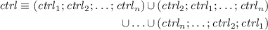
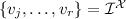
(Component). A component \(C=\,\)(ctrl, plant, cp) is defined as
-
ctrl is the discrete part without differential equations,
-
plant is a differential equation
 ,
, -
cp are deterministic assignments connecting ports of sub-components, and
-
 , correspondingly for \(BV(C_i)\).
 ,
, , correspondingly for
 If a component is atomic, i.e., not composed from sub-components, the port connections cp are empty (skip statement of no effect). The variables of a component are the sum of all used variables. We aim at components that can be analyzed in isolation and that communicate solely through ports. Global shared constants (read-only and thus not used for communication purposes) are included for convenience to share common knowledge for all components in a single place.
Definition 2
(Variable Restrictions). A system of components  is well-defined if
-
global variables
 are read-only and shared by all components:
 ,
, -
 such that no variable of other components can be read or written.
 are read-only and shared by all components:
 ,
, such that no variable of other components can be read or written.
Consider the robot collision avoidance system. Its global variables are the maximum obstacle speed S and the maximum difference  between two speed advisories, i.e.,
  . They can neither be bound in control nor plant, cf. Definition 2. The RC component’s controller picks a new demanded speed d that is not too far from the previous demanded speed \(d^-\). Since it is not composed from sub-components the \(cp_{rc}\) part is skip in Fig. 1. The obstacle’s controller chooses any speed \(s_{o}\) that does not exceed the maximum speed S. The plant ODE
  describes how the position of the obstacle changes according to its speed. Since the obstacle is an atomic component,
  is skip, cf. Fig. 1.
An interface defines how a component may interact with other components through its ports, what assumptions the component makes about its inputs, and what guarantees it provides for its outputs, see Definition 3.
Definition 3
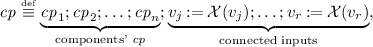
(Admissible Interface). An admissible interface \({{I}^{\varDelta }}\) for a component C is a tuple  with
with
-
 and
and  are disjoint sets of input- and output variables,
 -
 , i.e., input variables may not be bound in the component,
 -
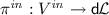 is a function specifying exactly one formula per input variable (i.e., input port), representing input requirements and assumptions,
 -
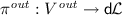 specifies output guarantees for output ports,
 -
 such that input formulas are local to their port,
 -
 is a set of \(\varDelta \)-port variables of unconnected public
  , and connected private
  , with
  , so
, so  ,
, -
 with
with 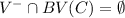 is a read-only set of variables storing the previous values of \(\varDelta \)-ports, disjoint from other interface variables
  ,
, -
 is a bijective function, assigning one variable to each \(\varDelta \)-port to store its previous value.
 and
and  are disjoint sets of input- and output variables,
 , i.e., input variables may not be bound in the component,
 is a function specifying exactly one formula per input variable (i.e., input port), representing input requirements and assumptions,
 specifies output guarantees for output ports,
 such that input formulas are local to their port,
 is a set of
  , and connected private
  , with
  , so
, so  ,
, with
with  is a read-only set of variables storing the previous values of
  ,
, is a bijective function, assigning one variable to each
 The definition is accordingly for vector-valued ports that share multiple variables along a single port, provided that each variable is part of exactly one vectorial port. This leads to multi-ports, which transfer the values of multiple variables, but have a single joint output guarantee/input assumption over the variables in the multi-port vector. Input assumptions are local to their port, i.e., no input formula can mention other input variables (which lets us reshuffle port ordering) nor any output variables (which prevents cyclic port definitions). Not all ports of a component need to be connected to other components; unconnected ports simply remain input/output ports of the resulting composite system.
Considering our example, the RC interface  from (1) contains one output port d in \(V^{out}\), where the robot can retrieve the demanded speed. The RC guarantees that the new demanded speed d will not deviate too far from the previous speed \({d^{-}}\), so
  . Since the current and the previous demanded speed are related, d is a \(\varDelta \)-port in \(V^{\varDelta }\) with its previous value \({d^{-}}\) in \({V^{-}}\) per pre.

3.2 Specification: Time and Delay
In a monolithic hybrid program with a combined plant for all components, time passes synchronously for all components and their ODEs evolve for the same amount of time. When split into separate components, the ODEs are split into separate plants too, thereby losing the connection of evolving for identical amounts of time. From the viewpoint of a single component, other plants reduce to discrete abstractions through input assumptions on \(\varDelta \)-ports. These input assumptions are phrased in terms of worst-case behavior (e.g., from the viewpoint of the robot, the obstacle may jump at most distance  between measurements because it lost a precise model). The robot’s ODE, however, still runs for some arbitrary time, which makes the measurements and the continuous behavior of the robot drift (i.e., robot and obstacle appear to move for different durations). To address this issue, we introduce delay as a way of ensuring that the changes are consistent with the time that passes in a component.
To unify the timing for all components of a system, we introduce a globally synchronized time t and a global variable \(t^{-}\) to store the time before each run of plant. Both are special global variables, which cannot be bound by the user, but only on designated locations specified through the contract, cf. Definition 4.
Definition 4
(Time). Let  be any number of components with variables according to Definition 2. When working with delay contracts, we assume
-
the global system time t changes with constant rate
 ,
, -
\(t^{-}\) is the initial plant time at the start of the current plant run,
-
 , thus clocks \(t, {t^{-}}\) are not written by a component.
 ,
, , thus clocks
 Let us continue our running example with the obstacle’s interface, which has one output port (providing the current obstacle position) that uses the introduced global time in its output property to restrict the obstacle’s position relative to its previous position and maximum speed, i.e.,

3.3 Proof Obligations: Change and Delay Contract
Contract compliance ties together components and interfaces by showing that a component guarantees the output changes that its interface specifies under the input assumptions made in the interface. Contract compliance further shows a local safety property, which describes the component’s desired safe states. For example, a safety property of a robot might require that the robot will not drive too close to the last measured position of the obstacle. Together with the obstacle’s output guarantee of not moving too far from its previous position, the local safety property implies a system-wide safety property (e.g., robot and obstacle will not collide), since we know that a measurement previously reflected the real position. Contract compliance can be verified using KeYmaera X [7].
In order to make guarantees about the behavior of a composed system we use the synchronized system time t to measure the delay \((t-t^{-})\) between controller runs in delay contract compliance proof obligations, cf. Definition 5.
Definition 5
(Contract Compliance). Let C be a component with its admissible interface \({{I}^{\varDelta }}\) (cf. Definition 3). Let formula \(\phi \) describe initial states of C and formula  the safe states, both over the component variables V(C). The output guarantees
  extend safety to
  . Change contract compliance
  of C with \({{I}^{\varDelta }}\) is defined as the
  formula:

and delay contract compliance  is defined as the
  formula:

where

are (vectorial) assignments to input ports satisfying input assumptions  and \(\varDelta \) are (vectorial) assignments storing previous values of \(\varDelta \)-port variables:

The order of the assignments in both in and \(\varDelta \) is irrelevant because the assignments are over disjoint variables and  are local to their port, cf. Definition 3. The function pre can be used throughout the component to read the initial value of a \(\varDelta \)-port. Since
  , Definitions 3 and 5 require that the resulting initial variable is not bound anywhere outside \(\varDelta \).
This notion of contracts crucially changes compared to [16] with respect to where ports are read and how change is modeled: reading from input ports at the beginning of a component’s loop body (i.e., before the controller runs) as in [16] may seem intuitive, but it would require severe restrictions to a component’s plant in order to make inputs and plant agree on duration. Instead, we prepare the next loop iteration at the end of the loop body (i.e., after plant), so that actual plant duration can be considered for computing the next input values.
Example: Change Contract. We continue the collision avoidance system with a change contract (2) according to Definition 5 for the RC from Fig. 1. The difference between speed advisories should be non-negative, whereas the output port’s previous value \({d^{-}}\) is bootstrapped from the current demanded speed d to guarantee contract compliance even without component execution, since non-deterministic repetitions can execute 0 times, so  . The RC guarantees that consecutive speed advisories are at most D apart, see
  ).
).

We verified the RC contract using KeYmaera X and thus know that the component is safe and complies with its interface. Compared to contracts with fixed ranges as in approaches [3, 16], we do not have to assume a global limit for demanded speeds d, but consider the previous advice \({d^{-}}\) as a reference value when calculating the next speed advice.
Example: Delay Contract. Change in obstacle position depends on speed and on how much time passed. Hence, we follow Definition 5 to specify the obstacle delay contract (3). For simplicity, assume that maximum speed S is non-negative and the obstacle stopped initially. As before, the previous position \(p^{-}_{o}\) is bootstrapped from the current position \({p_{o}}\), so  . We model an adversarial obstacle, which does not care about safety. Thus, the output property only guarantees that positions change at most by
  , which is a discrete abstraction of the obstacle’s physical movement. Such an abstraction can be found by solving the plant ODE or from differential invariants [24]. Again, we verified the obstacle’s contract compliance using KeYmaera X.

3.4 Proof Obligations: Compatible Parallel Composition
From components with verified contract compliance, we now compose systems and provide safety guarantees about them, without redoing system proofs. For this, Definition 6 introduces a quasi-parallel composition, where the discrete ctrl parts of the components are executed sequentially in any order, while the continuous plant parts run in parallel. The connected ports cp of all components are composed sequentially in any order, since the order of independent deterministic assignments (i.e., assignments having disjoint free and bound variables) is irrelevant. Such a definition is natural in  , since time only passes during continuous evolution in hybrid programs, while the discrete actions of a program do not consume time and thus happen instantaneously at a single real point in time, but in a specific order. The actual execution order of independent components in a real system is unknown, which we model with a non-deterministic choice between all possible controller execution orders. Values can be exchanged between components using \(\varDelta \)-ports; all other variables are internal to a single component, except global variables, which can be read everywhere, but never bound, and system time \(t, {t^{-}}\), which can be read everywhere, but only bound at specific locations fixed by the delay contract, cf. Definition 5. \(\varDelta \)-ports store their previous values in the composite component, regardless if connected or not. For all connected ports, Definition 6 replaces the non-deterministic assignments to open inputs (cf. in) with a deterministic assignment from the connected port (cf. cp). This represents an instantaneous and lossless interaction between components.
Definition 6
(Parallel Composition). Let \({C_{i}}=\mathrm{(ctrl_\textit{i}, plant_\textit{i}, cp_\textit{i})}\) denote components with their corresponding admissible interfaces

sharing only  and global times such that
  . Let further

be a partial (i.e., not every input must be mapped), injective (i.e., every output is only mapped to at most one input) function, connecting some inputs to some outputs, with domain  and image
  . The composition of n components and their interfaces
  is defined as:
-
controllers are executed in non-deterministic order of all the \(n!\) possible permutations of \(\{1,\ldots ,n\}\),
-
plants are executed in parallel, with evolution domain


-
port assignments are extended with connections for some
-
previous values
 are merged; connected ports become private
  ; unconnected ports remain public
  ,
, -
\({pre_{i}}\) are combined such that
 ,
, -
unconnected inputs
 and unconnected outputs
 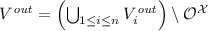 are merged and their requirements preserved
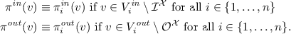


 are merged; connected ports become private
  ; unconnected ports remain public
  ,
, ,
, and unconnected outputs
  are merged and their requirements preserved
The order of port assignments is irrelevant because all sets of variables are disjoint and a port can only be either an input port or output port, cf. Definitions 1 and 3, and thus the assignments share no variables. This also entails that the merged pre, \({\pi ^{in}}\) and \({\pi ^{out}}\) are well-defined since  ,
,  , respectively
  , are disjoint between components by Definition 2.
The user provides component specifications  and a mapping function
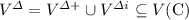
  , defining which output is connected to which input. The composed system of parallel components can be derived automatically from Definition 6. It follows that the set of variables of the composite component V(C) is the union of all involved components’ variable sets
  . The set of global variables \({V^{global}}\) contains all global variables in the system (i.e., in all components) and thus, its contents do not change. Since
  , this definition implies that internally connected \(\varDelta \)-ports \({V^{\varDelta i}}\) of sub-components, as well as the previous values \({V^{\varDelta +}}\) for all open \(\varDelta \)-ports are still stored. As a result, the current and previous values of \(\varDelta \)-ports can still be used internally in the composite, even when the ports are no longer exposed through the external interface of the composed system.
Returning to our running example of Fig. 1 the component  in (4) and interface
  in (5) result from parallel composition of the RC, the robot, and the obstacle. The robot controller follows the speed advice received on input port \(\hat{d}\) if the robot is at a safe distance from the obstacle position measured with input port \({\hat{p}_{o}}\); otherwise it stops. The robot plant changes the robot’s position according to its speed, where the controller executes at least every \(\varepsilon \) time-units. The robot’s input ports are connected to the RC’s and obstacle’s output ports.Footnote 2


During composition, the tests guarding the input ports of an interface are replaced with a deterministic assignment modeling the port connection of the components, which is only safe if the respective output guarantees and input assumptions match. Hence, in addition to contract compliance, users have to show compatibility of components as defined in Definition 7.
Definition 7
(Compatible Composite). A composite of \(n\) components with interfaces  is a compatible composite iff
  formula

is valid over (vectorial) equalities and assignments for input ports  from
from  . We call
  the compatibility proof obligation for the interfaces
  and say the interfaces
  are compatible (with respect to
  ) if
) if  is valid for all i.
Components are compatible if the output properties imply the input properties of connected ports. Compatibility guarantees that handing an output port’s value over to the connected input port ensures that the input port’s input assumption \({\pi ^{in}}\) holds, which is no longer checked explicitly by a test, so  . To achieve local compatibility checks for pairs of connected ports, instead of global checks over entire component models, we restrict output guarantees, respectively input assumptions to the associated output ports, respectively input ports (cf. Definition 3). In our example, the robot and the obstacle, respectively the RC are compatible, as witnessed by proofs of
  and
and  , cf. [17].
3.5 Transferring Local Component Safety to System Safety
After verifying contract compliance and compatibility proof obligations, Theorem 1 below ensures that the safety properties in component contracts imply safety of the composed system. Thus, to ensure a safety property of the monolithic system, we no longer need a (probably huge) monolithic proof, but can apply Theorem 1 (proof available in [17]).
Theorem 1
(Composition Retains Contracts). Let \({C_{1}}\) and \({C_{2}}\) be components with admissible interfaces  and
and  that are delay contract compliant (cf. Definition 5) and compatible with respect to
  (cf. Definition 7). Initially, assume
  to bootstrap connected ports. Then, if the side condition (6) holds (\(\varphi _i\) is the loop invariant used to prove the component’s contract)

for all components \({C_{i}}\), the parallel composition  then satisfies the contract (7) with \(\mathrm{in}\), \(\mathrm{cp}\), \(\mathrm{ctrl}\), and \(\mathrm{plant}\) according to Definition 6:

The composite contract’s precondition \(\phi ^{p}\) ensures that the values of connected ports are consistent initially. Side condition (6) shows that a component already produces the correct output from just its ctrl and plant; preparing the port inputs for the next loop iteration does not change the current output.
The side condition (6) is trivially true for components without output ports, since  . For atomic components without input ports, the proof of (6) automatically follows from the contract proof, since in; cp is empty. Because of the precondition \(\phi ^{p}\) and because cp is executed after every execution of the main loop (cf. Definition 5), we know that the values of connected input and output ports coincide in the safety property, as one would expect. Thus, for instance, if the local safety property of a single component mentions an input port (e.g.,
  , we can replace the input port with the original value as provided by the output port for the composite safety property (e.g.,
  ). Theorem 1 easily extends to n components (cf. proof sketch in [17]) and also holds for change contracts. A change port cannot be attached to a delay port and vice versa.
Going back to our example, the overall system property of our collision avoidance system follows from Theorem 1, given the local safety property of the robot, the change contract compliance of the RC, the delay contract compliance of the obstacle, and the compatibility of the connections. Since we verified all component contracts as well as the compatibility proof obligations and since the components with output ports are atomic and have no input ports (i.e., the side condition holds), safety of the collision avoidance system follows.
Automation. We implemented the proof steps of Theorem 1 as a KeYmaera X tactic, which automatically reduces a system safety proof to separate proofs about componentsFootnote 3. This gave us the best of the two worlds: the flexibility of reasoning with components that our Theorem 1 provides, together with the soundness guarantees we inherit from KeYmaera X, which derives proofs by uniform substitution from axioms [25]. This is to be contrasted with the significant soundness-critical changes we would have to do if we were to add Theorem 1 as a built-in rule into the KeYmaera X prover core. Uniform substitution guarantees, e.g., that the subtle conditions on how and where input and output variables can be read or written in components are checked correctly.
4 Case Studies
To evaluate our approach (See footnote 3), we use the running example of a remote-controlled robot (RC robot) and revisit prior case studies on the European Train Control System (i.e., ETCS) [26], two-component robot collision avoidance (i.e., Robix) [13], and adaptive cruise control (i.e., LLC) [10]. In ETCS, a radio-block controller (RBC) communicates speed limits to a train, i.e., it requires the train to have at most speed \(d\) after some point \(m\). The RBC multi-port change contract relates distances \(m,m^-\) and demanded speeds \(d,d^-\) in input assumptions/output guarantees of the form \(d \ge 0 \wedge {(d^-)}^2 - d^2 \le 2 b (m-m^-) \wedge \textit{state}=\textit{drive} \), thus avoiding physically impossible maneuvers.
In Robix, a robot measures the position of a moving obstacle with a maximum speed S. The obstacle guarantees to not move further than  in either axis between measurements, using a delay contract.
In LLC, a follower car measures both speed \(v_l\) and position \(x_l\) of a leader car, with maximum acceleration \(A\) and braking capabilities \(B\). Hence, we use a multi-port delay contract with properties of the form  tying together speed change and position progress.
Table 1 summarizes the experimental results of the component-based approach in comparison to monolithic models in terms of duration and degree of proof automation. The column Contract describes the kind of contract used in the case study (i.e., multiport, delay contract or change contract), as well as whether or not the models use non-linear differential equations. The column Automation indicates fully automated proofs with checkmarks; it indicates the number of built-in tactics composed to form a proof script when user input is required. The column Duration compares the proof duration, using Z3 [14] as a back-end decision procedure to discharge arithmetic. The column \(Sum\) sums up the proof durations for the components (columns \(C_1\) and \(C_2\)) and Theorem 1 (column Th. 1, i.e., checking compatibility, condition (6) and the execution of our composition proof). Checking the composition proof is fully automated, following the proof steps of Theorem 1.
All measurements were conducted on an Intel i7-6700HQ CPU@2.6 GHz with 16 GB memory. In summary, the results indicate that our approach verification leads to performance improvements and smaller user-provided proof scripts.
5 Related Work
We group related work into hybrid automata, hybrid process algebras, and hybrid programs.
Hybrid Automata and Assume-Guarantee Reasoning. Hybrid automata [1] can be composed in parallel. However, the associated verification procedure (i.e., verify that a formula holds throughout all runs of the automaton) is not compositional, but requires verification of the exponential product automaton [1]. Thus, for a hybrid automaton it is not sufficient to establish a property about its parts in order to establish a property about the automaton. We, instead, decompose verification into local proofs and get system safety automatically. Hybrid I/O automata [11] extend hybrid automata with a notion of external behavior. The associated implementation relation (i.e., if automaton \(A\) implements automaton \(B\), properties verified for \(B\) also hold for \(A\)) is respected by their composition operation in the sense that if \(A_1\) implements \(A_2\), then the composition of \(A_1\) and \(B\) implements the composition of \(A_2\) and \(B\). Hybrid (I/O) automata are mainly verified using reachability analysis. Therefore, techniques to prevent state-space explosion are needed, like assume-guarantee reasoning (AGR, e.g., [3, 6, 9]), which was developed to decompose a verification task into subtasks. In [6], timed transition systems are used to approximate a component’s behavior by discretization. These abstractions are then used in place of the more complicated automata to verify refinement properties. The implementation of their approach is limited to linear hybrid automata. In analogy, we discretize plants to delay contracts; however, in our approach, contracts completely replace components and do not need to retain simplified transition systems. A similar AGR rule is presented in [9], where the approximation drops continuous behaviors of single components entirely. As a result, the approach only works when the continuous behavior is irrelevant to the verified property, which rarely happens in CPS. Our change and delay contracts still preserve knowledge about continuous behavior. The AGR approach of [3] uses contracts consisting of input assumptions and output guarantees to verify properties about single components: a component is an abstraction of another component if it has a stricter contract. The approach is restricted to constant intervals, i.e., static global contracts as in [16].
In [5], a component-based design framework for controllers of hybrid systems with linear dynamics based on hybrid automata is presented. It focuses on checking interconnections of components: alarms propagated by an out-port must be handled by the connected in-ports. We, too, check component compatibility, but for contracts, and focus on transferring proofs from components to the system level. We provide parallel composition, while [5] uses sequential composition. The compositional verification approach in [2] bases on linear hybrid automata using invariants to over-approximate component behavior and interactions. However, interactions between components are restricted to synchronization. (i.e., no variable state can be transferred between components).
In summary, aforementioned approaches are limited to linear dynamics [5] or even linear hybrid automata [2], use global contracts [3], focus on sequential composition [5] or rely on reachability analysis, over-approximation and model checking [3, 6, 9]. We, in contrast, focus on theorem proving in  , using change and delay contracts and handle non-linear dynamics and parallel composition. Most crucially, we focus on transfer of safety properties from components to composites, while related approaches are focused on property transfer between different levels of abstraction [3, 6, 9].
Hybrid process algebras are compositional modeling formalisms for the description of behavior and interaction of processes, based on algebraic equations. Examples are Hybrid \(\chi \) [27], HyPA [18] or the \(\varPhi \)-Calculus [28]. Although the modeling is compositional, for verification purposes the models are again analyzed using simulation or reachability analysis in a non-compositional fashion (e.g., Hybrid \(\chi \) using PHAVer [30], HyPA using HyTech [12], \(\varPhi \)-Calculus using SPHIN [29]), while we focus on exploiting compositionality in the proof.
Hybrid Programs. Quantified hybrid programs enable a compositional verification of hybrid systems with an arbitrary number of components [20], if they all have the same structure (e.g., many cars, or many robots). They were used to split monolithic hybrid program models into smaller parts to show that adaptive cruise control prevents collisions for an arbitrary number of cars on a highway [10]. We focus on different components. Similarly, the approach in [15] presents a component-based approach limited to traffic flow and global contracts.
Our approach extends [16], which was restricted to contracts over constant ranges. Such global contracts are well-suited for certain use cases, where the change of a port’s value does not matter for safety, such as the traffic flow models of [15]. However, for systems such as the remote-controlled robot obstacle avoidance from our running example (cf. Sect. 3.1), which require knowledge about the change of certain values, global contracts only work for considerably more conservative models (e.g., robot and obstacle must stay in fixed globally known regions, since the obstacle’s last position is unknown). Contracts with change and delay allow more liberal component interaction.
6 Conclusion and Future Work
Component-based modeling and verification for hybrid systems splits monolithic system verification into proofs about components with local responsibilities. It reduces verification effort compared to proving monolithic models, while change and delay contracts preserve crucial properties about component behavior to allow liberal component interaction.
Change contracts relate a port’s previous value to its current value (i.e., the change since the last port transmission), while delay contracts additionally relate to the delay between measurements. Properties of components, described by component contracts and verified using KeYmaera X, transfer to composed systems of multiple compatible components without re-verification of the entire system. We have shown the applicability of our approach on a running example and three existing case studies, which furthermore demonstrated the potential reduction of verification effort. We implemented our approach as a KeYmaera X tactic, which automatically verifies composite systems based on components with verified contracts without increasing the trusted prover core.
For future work, we plan to (i) introduce further composition operations (e.g., error-prone transmission), and (ii) provide support for system decomposition by discovery of output properties (i.e., find abstraction for port behavior).
Notes
- 1.
Bound variables of a hybrid program are all those that may potentially be written to, while free variables are all those that may potentially be read [25].
- 2.
For the detailed robot component
 and interface
  , see [17].
 - 3.
Implementation and full models available online at http://www.cs.cmu.edu/~smitsch/resource/fase17.
 and interface
  , see [
References
Alur, R., Courcoubetis, C., Henzinger, T.A., Ho, P.-H.: Hybrid automata: an algorithmic approach to the specification and verification of hybrid systems. In: Grossman, R.L., Nerode, A., Ravn, A.P., Rischel, H. (eds.) HS 1991-1992. LNCS, vol. 736, pp. 209–229. Springer, Heidelberg (1993). doi:10.1007/3-540-57318-6_30
Aştefănoaei, L., Bensalem, S., Bozga, M.: A compositional approach to the verification of hybrid systems. In: Ábrahám, E., Bonsangue, M., Johnsen, E.B. (eds.) Theory and Practice of Formal Methods. LNCS, vol. 9660, pp. 88–103. Springer, Cham (2016). doi:10.1007/978-3-319-30734-3_8
Benvenuti, L., Bresolin, D., Collins, P., Ferrari, A., Geretti, L., Villa, T.: Assume-guarantee verification of nonlinear hybrid systems with Ariadne. Int. J. Robust Nonlinear Control 24(4), 699–724 (2014)
Bohrer, B., Rahli, V., Vukotic, I., Völp, M., Platzer, A.: Formally verified differential dynamic logic. In: Bertot, Y., Vafeiadis, V. (eds.) Proceedings of the 6th ACM SIGPLAN Conference on Certified Programs and Proofs, pp. 208–221. ACM (2017)
Damm, W., Dierks, H., Oehlerking, J., Pnueli, A.: Towards component based design of hybrid systems: safety and stability. In: Manna, Z., Peled, D.A. (eds.) Time for Verification. LNCS, vol. 6200, pp. 96–143. Springer, Heidelberg (2010). doi:10.1007/978-3-642-13754-9_6
Frehse, G., Han, Z., Krogh, B.: Assume-guarantee reasoning for hybrid I/O-automata by over-approximation of continuous interaction. In: 43rd IEEE Conference on Decision and Control, CDC, vol. 1, pp. 479–484 (2004)
Fulton, N., Mitsch, S., Quesel, J.-D., Völp, M., Platzer, A.: KeYmaera X: an axiomatic tactical theorem prover for hybrid systems. In: Felty, A.P., Middeldorp, A. (eds.) CADE 2015. LNCS (LNAI), vol. 9195, pp. 527–538. Springer, Cham (2015). doi:10.1007/978-3-319-21401-6_36
Henzinger, T.A.: The theory of hybrid automata. In: Proceedings, 11th Annual IEEE Symposium on Logic in Computer Science, pp. 278–292. IEEE Computer Society (1996)
Henzinger, T.A., Minea, M., Prabhu, V.: Assume-guarantee reasoning for hierarchical hybrid systems. In: Di Benedetto, M.D., Sangiovanni-Vincentelli, A. (eds.) HSCC 2001. LNCS, vol. 2034, pp. 275–290. Springer, Heidelberg (2001). doi:10.1007/3-540-45351-2_24
Loos, S.M., Platzer, A., Nistor, L.: Adaptive cruise control: hybrid, distributed, and now formally verified. In: Butler, M., Schulte, W. (eds.) FM 2011. LNCS, vol. 6664, pp. 42–56. Springer, Heidelberg (2011). doi:10.1007/978-3-642-21437-0_6
Lynch, N.A., Segala, R., Vaandrager, F.W.: Hybrid I/O automata. Inf. Comput. 185(1), 105–157 (2003)
Man, K.L., Reniers, M.A., Cuijpers, P.J.L.: Case studies in the hybrid process algebra Hypa. Int. J. Softw. Eng. Knowl. Eng. 15(2), 299–306 (2005)
Mitsch, S., Ghorbal, K., Platzer, A.: On provably safe obstacle avoidance for autonomous robotic ground vehicles. In: Newman, P., Fox, D., Hsu, D. (eds.) Robotics: Science and Systems IX (2013)
de Moura, L., Bjørner, N.: Z3: an efficient SMT solver. In: Ramakrishnan, C.R., Rehof, J. (eds.) TACAS 2008. LNCS, vol. 4963, pp. 337–340. Springer, Heidelberg (2008). doi:10.1007/978-3-540-78800-3_24
Müller, A., Mitsch, S., Platzer, A.: Verified traffic networks: component-based verification of cyber-physical flow systems. In: 18th International Conference on Intelligent Transportation Systems, pp. 757–764 (2015)
Müller, A., Mitsch, S., Retschitzegger, W., Schwinger, W., Platzer, A.: A component-based approach to hybrid systems safety verification. In: Ábrahám, E., Huisman, M. (eds.) IFM 2016. LNCS, vol. 9681, pp. 441–456. Springer, Cham (2016). doi:10.1007/978-3-319-33693-0_28
Müller, A., Mitsch, S., Retschitzegger, W., Schwinger, W., Platzer, A.: Change and delay contracts for hybrid system component verification. Technical report CMU-CS-17-100, Carnegie Mellon (2017)
Cuijpers, P.J.L., Reniers, M.A.: Hybrid process algebra. J. Log. Algebr. Program. 62(2), 191–245 (2005)
Platzer, A.: Differential-algebraic dynamic logic for differential-algebraic programs. J. Log. Comput. 20(1), 309–352 (2010)
Platzer, A.: Quantified differential dynamic logic for distributed hybrid systems. In: Dawar, A., Veith, H. (eds.) CSL 2010. LNCS, vol. 6247, pp. 469–483. Springer, Heidelberg (2010). doi:10.1007/978-3-642-15205-4_36
Platzer, A.: A complete axiomatization of quantified differential dynamic logic for distributed hybrid systems. Logical Methods Comput. Sci. 8(4), 1–44 (2012)
Platzer, A.: The complete proof theory of hybrid systems. In: Proceedings of the 27th Annual IEEE Symposium on Logic in Computer Science, pp. 541–550. IEEE Computer Society (2012)
Platzer, A.: Logics of dynamical systems science. In: Proceedings of the 27th Annual IEEE Symposium on Logic in Computer Science, pp. 13–24. IEEE Computer Society (2012)
Platzer, A.: The structure of differential invariants and differential cut elimination. Logical Methods Comput. Sci. 8(4), 1–38 (2012)
Platzer, A.: A complete uniform substitution calculus for differential dynamic logic. J. Autom. Reas. 1–47 (2016). doi:10.1007/s10817-016-9385-1
Platzer, A., Quesel, J.-D.: European train control system: a case study in formal verification. In: Breitman, K., Cavalcanti, A. (eds.) ICFEM 2009. LNCS, vol. 5885, pp. 246–265. Springer, Heidelberg (2009). doi:10.1007/978-3-642-10373-5_13
Schiffelers, R.R.H., van Beek, D.A., Man, K.L., Reniers, M.A., Rooda, J.E.: Formal semantics of hybrid Chi. In: Larsen, K.G., Niebert, P. (eds.) FORMATS 2003. LNCS, vol. 2791, pp. 151–165. Springer, Heidelberg (2004). doi:10.1007/978-3-540-40903-8_12
Rounds, W.C., Song, H.: The Ö-calculus: a language for distributed control of reconfigurable embedded systems. In: Maler, O., Pnueli, A. (eds.) HSCC 2003. LNCS, vol. 2623, pp. 435–449. Springer, Heidelberg (2003). doi:10.1007/3-540-36580-X_32
Song, H., Compton, K.J., Rounds, W.C.: SPHIN: a model checker for reconfigurable hybrid systems based on SPIN. Electr. Notes Theor. Comput. Sci. 145, 167–183 (2006)
Xinyu, C., Huiqun, Y., Xin, X.: Verification of hybrid Chi model for cyber-physical systems using PHAVer. In: Barolli, L., You, I., Xhafa, F., Leu, F.Y., Chen, H.C. (eds.) 7th International Conference on Innovative Mobile and Internet Services in Ubiquitous Computing, pp. 122–128. IEEE Computer Society (2013)
Author information
Authors and Affiliations
Corresponding author
Editor information
Editors and Affiliations
Rights and permissions
Copyright information
© 2017 Springer-Verlag GmbH Germany
About this paper
Cite this paper
Müller, A., Mitsch, S., Retschitzegger, W., Schwinger, W., Platzer, A. (2017). Change and Delay Contracts for Hybrid System Component Verification. In: Huisman, M., Rubin, J. (eds) Fundamental Approaches to Software Engineering. FASE 2017. Lecture Notes in Computer Science(), vol 10202. Springer, Berlin, Heidelberg. https://doi.org/10.1007/978-3-662-54494-5_8
Download citation
DOI: https://doi.org/10.1007/978-3-662-54494-5_8
Published:
Publisher Name: Springer, Berlin, Heidelberg
Print ISBN: 978-3-662-54493-8
Online ISBN: 978-3-662-54494-5
eBook Packages: Computer ScienceComputer Science (R0)
