A Minor Note on Obtaining Simpler iO Constructions via Depleted Obfuscators

Abstract

This paper puts forth a simple construction for indistinguishability obfuscation ($\textsf{iO}$) for general circuits. The scheme is obtained from four main ingredients: (1) selectively indistinguishably-secure functional encryption for general circuits having its encryption procedure in the complexity class $\textsf{NC}^1$; (2) universal circuits; (3) puncturable pseudorandom functions having evaluation in $\textsf{NC}^1$; (4) indistinguishably-secure affine-determinant programs, a notion that particularizes $\textsf{iO}$ for specific circuit classes and acts as “depleted” obfuscators. The scheme can be used to build $\textsf{iO}$ for all polynomial-sized circuits in a simplified way.

Appendices

A Puncturable PRFs with Evaluations in $\textsf{NC}^1$

In this part, we provide evidence that a particular version of the constrained PRF from [11] – namely the “toy” puncturable PRF informally introduced by Boneh, Kim and Montgomery in [8, Section 1] – admits an $\textsf{NC}^1$ circuit representation of the evaluation function. This informal scheme is chosen for space reasons, and also for simplicity (avoiding the usage of universal circuits in its description). The notations that are used in this part are as follows: $|\textsf{inp}|$ stands for the length of the input string, $\lambda$ stands for the security parameter, n and m stand for the dimensions of the matrix used in the construction, q stand for the $\textsf{LWE}$ modulus.

• given the unary description of the security parameter $\lambda$:

  1. Sample acolumn vector:

  2. Sample $|\textsf{inp}|$ matrices $\textbf{B}_i$ of dimensions $n \times m$ uniformly at random over $\mathbb {Z}_q^{n \times m}$, for all $i \in [|\textsf{inp}|]$. That is:

  3. Sample 2 matrices $\textbf{A}_0, \textbf{A}_1$ as before:

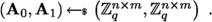
  4. Set as secret key: $\textsf{k}\leftarrow \left( \textbf{s},~ \textbf{B}_1,~ \ldots ,~ \textbf{B}_{|\textsf{inp}|},~ \textbf{A}_0,~ \textbf{A}_1 \right) ~.$

• To evaluate input $\textsf{inp}$ under $\textsf{pPRF}$ key $\textsf{k}$, proceed as follows

  1. Use the $\textsf{PK}_\textsf{Eval}$ evaluation algorithm from [11] (detailed below) in order to publicly compute a matrix $\textbf{A}_\textsf{eq}$.

  2. Compute: $Y \leftarrow \textbf{s}^\top \cdot \textbf{A}_\textsf{eq}~.$

  3. Return $\lfloor Y \rceil ~,$ where $\lfloor \cdot \rceil$ is a rounding function: $\lfloor \cdot \rceil : \mathbb {Z}_q \rightarrow \mathbb {Z}_p$ that maps $x \rightarrow \lfloor x\cdot (p/q)\rceil$, i.e. the argument x is multiplied with p/q and the result is rounded (over reals).

• 

  1. Return the punctured key for $\textsf{inp}^* = (\textsf{inp}^*_1, \ldots , \textsf{inp}^*_{|\textsf{inp}|}) \in \{0,1\}^{|\textsf{inp}|}$ as

  $$ \textsf{k}^* \leftarrow \left( \textsf{inp}^*, \left\{ \textbf{s}^\top \cdot \left( \textbf{A}_k + k \cdot \textbf{G}\right) + \textbf{e}_k\right\} _{k \in \{0,1\}}, \left\{ \textbf{s}^\top \cdot \left( \textbf{B}_k + \textsf{inp}^*_k \cdot \textbf{G}\right) + \textbf{e}^*_k\right\} _{k=1}^{|\textsf{inp}^*|} \right) ~. $$

• To evaluate in the punctured point:

  1. Compute the encoding evaluation (detailed below) over the punctured key and obtain Y: $Y \leftarrow \textbf{s}^\top \cdot \left( \textbf{A}_\textsf{eq}+ \textsf{eq}(\textsf{inp}^*,\textsf{inp}) \cdot \textbf{G}\right) + \textbf{e}'~.$

  2. Return $\lfloor Y \rceil$ where $\lfloor \cdot \rceil$ is the same rounding function used by the normal evaluation.

Observe that when $\textsf{eq}(\textsf{inp}^*, \textsf{inp})=0$, the value Y computed in punctured evaluation is in fact $\textbf{s}^\top \cdot \textbf{A}_\textsf{eq}+ \textbf{e}'$. The correctness and security are based on the constrained PRF scheme from [11], hence we ignore them herein. We focus on the runtime analysis of the punctured evaluation algorithm. In doing so, we need the public and the encoding evaluation algorithm.

1.1 A.1 The Encoding Evaluation Algorithm for the $\textsf{pPRF}$ in [11]

Consider a circuit composed from the universal set of gates: AND and NOT.

AND Gates: let $g_{u,v,w}$ be and AND gate, where u and v denote the input wires while w denotes the output. Let $\textbf{y}_u = \textbf{s}^\top \cdot \left( \textbf{A}+ x_u \cdot \textbf{G}\right) + \textbf{u}$ and $\textbf{y}_v = \textbf{s}^\top \cdot \left( \textbf{A}+ x_v \cdot \textbf{G}\right) + \textbf{v}$ where $x_u$ and $x_v$ denote the value of wires u and v corresponding to same input. The evaluation over encodings computes:

$$\begin{aligned} \textbf{y}_w \leftarrow x_u \cdot \textbf{y}_v - \textbf{y}_u \cdot \textbf{G}^{-1}(\textbf{A}_v)~. \end{aligned}$$

(5)

which will be a valid encoding corresponding to the value of w.

NOT Gates: we reuse similar notations for gates as per the previous case, with $g_{u,w}$ being a not gate and input wire is u, and $\textbf{y}_0$ is an encoding corresponding to the value 0:

$$\begin{aligned} \textbf{y}_w \leftarrow \textbf{y}_0 - \textbf{y}_u~. \end{aligned}$$

(6)

1.2 A.2 Punctured Evaluation’s Parallel Complexity

Here we scrutinize the parallel efficiency of the gate evaluation corresponding to the equality function:

$$\begin{aligned} \textsf{eq}(\textsf{inp}^*, \textsf{inp}) {:}{=}{\left\{ \begin{array}{ll} 1, \text { if } \textsf{inp}= \textsf{inp}^* \\ 0, \text { otherwise } \end{array}\right. } \end{aligned}$$

(7)

An unoptimized circuit that implements the $\textsf{eq}$ function is built as follows:

• 1. use a gadget matrix that returns the boolean value of $\textsf{inp}^*_i {\mathop {=}\limits ^{?}}\textsf{inp}_i$ for some input position $i \in [|\textsf{inp}|]$. This gadget matrix can be implemented as

  $$\begin{aligned} \text {NOT}\left( \left( \text {NOT} \left( \textsf{inp}^*_i\text {AND}\textsf{inp}_i \right) \right) \text {AND} \left( \text {NOT} \left( (\text {NOT}~\textsf{inp}^*_i) \text {AND} (\text {NOT}~\textsf{inp}_i) \right) \right) \right) \end{aligned}$$

  (8)

  Thus the depth of this gadget is 5, and on each of the 5 levels further $\textsf{LWE}$-related operations are to be performed.

• 2. use a full-binary tree style of circuit consisting of AND gates that outputs $\bigwedge _{i=1}^{|\textsf{inp}|}(\textsf{inp}^*_i {\mathop {=}\limits ^{?}}\textsf{inp}_i)$. Clearly, this circuit has $\lceil \log _2(|\textsf{inp}|) \rceil$ levels.

Henceforth, the circuit that computes the evaluation (obtained by applying the construction in step 2 on top of the “gadget” circuit) has depth $\le c \cdot \log _2(|\textsf{inp}|)$ for some constant c. The matrix multiplication involved in the computation of an AND gate, the values of $\textbf{G}^{-1}(\textbf{A}_0)$ and $\textbf{G}^{-1}(\textbf{A}_1)$ can be pre-stored, the costly part being a vector $\times$ matrix multiplication. The inner, $\textsf{LWE}$-related computations within the punctured evaluation algorithm are in $\textsf{NC}^1$, as for other constructions using $\textsf{LWE}$ tuples, (see for instance [2]). Further details on the complexity of circuits implementing addition/multiplication for elements in $\mathbb {F}_q$ are given in [23, Section 8]). Thus, we can assume that the there exists puncturable $\textsf{PRF}$s having their punctured evaluation circuit in $\textsf{NC}^1$ (as expected, also, by [25]).

B GKPVZ13’s Encryption Procedure is in $\textsf{NC}^1$

In this section, we provide an informal argument for the existence of $\textsf{FE}$ schemes having their encryption procedure in $\textsf{NC}^1$ (an assumption used in [25]). The notation used herein are independent from the ones used in other sections.

The FE Scheme from [17]. Goldwasser et al.’s proposal is to regard FE for circuits with a single-bit of output from the perspective of homomorphic operations. Their scheme’s encryption procedure proceeds as follows: (1) Samples on the fly keys for an $\textsf{FHE}$ scheme – namely $(\textsf{hpk}, \textsf{hsk})$ – and encrypts the input $\textsf{m}$ bitwise; let $\varPsi$ stand for the FHE ciphertext. (2) Then, the scheme makes use of Yao’s garbling protocol $\textsf{GS}$; this is employed to garble the circuit “$\textsf{FHE}.\textsf{Dec}(\textsf{hsk}, \cdot )$” and obtain two labels $L_i^0, L_i^1$ for each bit in the decomposition of $\varPsi$; (3) Finally, the scheme encrypts $\varPsi$, as well as $\textsf{hpk}$ under a set of $\textsf{ABE}$ public keys (in fact two-outcome ABEs are used). In some sense, $\varPsi$ corresponds to an attribute: if $\mathscr {C}_{f_i}(\varPsi )=0$ a label $L_i^0$ is revealed. Else, the label $L_i^1$ is returned.

For [17], a functional key for a circuit is nothing more than an $\textsf{ABE}$ key issued for the “$\textsf{FHE}.\textsf{Eval}$” circuit. The trick is that one decrypts an $\textsf{ABE}$ ciphertext with an $\textsf{ABE}$ key; this translates to applying $\textsf{FHE}.\textsf{Eval}$ over an $\textsf{FHE}$ ciphertext. Given the $\textsf{ABE}$ ciphertext encrypts $L_i^0, L_i^1$, depending on the output value (a bit b), the label $L_i^b$ is returned. After the labels are recovered, they can be used to feed the garbled circuit (included in the ciphertext); the decryptor evaluates and obtains (informally) $\textsf{FHE}.\textsf{Dec}(f(\varPsi ))$, thus yielding the expected output in a functional manner. Therefore, it is natural to set the master keys of the FE scheme as only the $\textsf{ABE}$s’ $\textsf{msk}$ and $\textsf{mpk}$. The total number of ABE keys to be sampled is determined by the length of the FHE ciphertext.

1.1 B.1 Attribute-Based Encryption

When we consider a key-policy setting, a decryption key of an ABE must be generated for one Boolean predicate $P : \{0,1\}^\lambda \rightarrow \{0,1\}$. A ciphertext of an ABE in this setting is the encryption of a set of attributes $\alpha$ over $\{0,1\}^\lambda$ and of some plaintext $\textsf{m}\in \{0,1\}^\gamma$. ABE’s correctness specifies that having a decryption key enables to recover the plaintext as long as $P(\alpha )=1$.

Instantiation of ABE. The seminal work of Gorbunov et al. [19] puts forward attribute-based encryption schemes for comprehensive classes of circuits. We review their construction, as it will serve in the circuit complexity analysis for this work. Our description is top-down: we describe the ABE scheme, and then review the TOR framework (their Two-to-One Recoding scheme).

Fig. 3.

In this section, $\ell$ stands for the FHE’s ciphertext’s length, while $\textsf{FHE}.\textsf{Eval}_f^i:\mathcal {K} \times \{0,1\}^{n \cdot \ell } \rightarrow \{0,1\}$ stands for a function that applies $\mathscr {C}_f$ on the encrypted input.

Attribute-Based Encryption from General Circuits. A key-policy ABE is presented in [19]. The main idea consists in evaluating on the fly a given circuit. The bitstring representing the attributes – say $\alpha$ – is known a priori, as well as the topology of the circuit – say $\phi$ – to be evaluated.

For each bit $\alpha _i$ in $\alpha$, there are two public keys associated – say $(\textsf{mpk}_i^0, \textsf{mpk}_i^1)$ – corresponding to 0 and 1. A vector $\textbf{s}\in \mathbb {F}_q^m$ is sampled uniformly at random, and encoded under the $\textsf{mpk}_i^{\alpha _i}$ as $\textsf{mpk}_i^{\alpha _i} \cdot \textbf{s}+ \text {noise}$. Then, the circuit $\phi$ is evaluated on these encodings. The crux point consists of a recoding procedure, which ensures that at the next level, $\textbf{s}$ is “recoded” under the next public key corresponding to the current gate. By keeping evaluating in such a way, the final output will be an encoding of $\textbf{s}$ under a circuit-dependent key $\textsf{pk}_{out}$. The encoding of the form $\textsf{pk}_{out} \cdot \textbf{s}+ \text {noise}$ is then used to recover the (symmetrically-)encrypted input X. We detail these procedures in what follows:

• $\textsf{Setup}(1^\lambda )$: consists of $\ell$ pairs of public keys, where $\ell$ is the length of the supported attributes $\alpha$: $\begin{pmatrix} \textsf{mpk}^0_1~~ &{} \textsf{mpk}^0_2~~ &{}~~ \ldots &{}~~ \textsf{mpk}^0_\ell \\ \textsf{mpk}^1_1~~ &{} \textsf{mpk}^1_2~~ &{}~~ \ldots &{}~~ \textsf{mpk}^1_\ell \end{pmatrix}$

  An additional key $\textsf{mpk}_{out}$ is sampled. Concretely, each $\textsf{mpk}_i^b$ corresponds to $\textbf{A}_i^b \in \mathbb {Z}_q^{n \times m}$. The master secret key consists of $2 \cdot n$ trapdoor matrices, which are described in the TOR subsection (see below).

• $\textsf{KeyGen}(\textsf{msk}, \phi )$: considering the circuit representation of $\phi :\{0,1\}^n \rightarrow \{0,1\}$. Each wire in the circuit is associated with two public keys, corresponding to a 0 and a 1. For each gate $g_{u,v,w}$, a table consisting of 4 recoding keys are generated: $rk^w_{g(\alpha , \beta )}$ for $g^w_{\alpha , \beta }$ the value of the gate under inputs $\alpha ,\beta \in \{0,1\}$.

  Based on the value of the gate applied on the inputs received from the attribute (which is known in plain) a recoding key is chosen. This recoding key is then used to recode the value of $\textbf{s}$ under the new public key.

• $\textsf{Enc}(\textsf{mpk}, X, \alpha )$: encrypting X means sampling a random vector and based on the decomposition of $\alpha$, obtaining the encodings of $\textbf{s}$ under $\textsf{mpk}_i^{\alpha _i}$.

  Finally, the input X itself is encrypted – via a semantic secure symmetric scheme – under Encode$(\textsf{mpk}_{out},s)$, which acts as a key. Thus, the ciphertext consists of $\left( \alpha , \left\{ \text {Encode}(\textsf{mpk}_i^{\alpha _i} \cdot \textbf{s}+ e_i) \right\} _{i=1}^n, \textsf{SE}.\textsf{Enc}(\text {Encode}(\textsf{mpk}_{out},s),X) \right) .$

• $\textsf{Dec}(\textsf{CT}, \textsf{sk}_\phi )$: the decryption procedure evaluates the circuit given the encodings and according to the attributes, and recovers $\text {Encode}(\textsf{pk}_{out},s)$. This is then used to recover X.

Two-to-One Recodings. The beautiful idea in [19] stems in the Two-To-One Recoding mechanism. The crux point is to start with two LWE tuples of the form $\textbf{A}_1 \cdot \textbf{s}+ \textbf{e}_1~~\text {and}~~\textbf{A}_2 \cdot \textbf{s}+ \textbf{e}_2$ and “recode” them under a new “target” matrix $\textbf{A}_{tgt}$. The outcome is indeed a recoding of $\textbf{s}$: $\textbf{A}_{tgt} \cdot \textbf{s}+ \textbf{e}_{tgt}~.$ In doing so, the recoding mechanism uses two matrices, $\textbf{R}_1, \textbf{R}_2$, such that $\textbf{A}_1 \cdot \textbf{R}_1 + \textbf{A}_2 \cdot \textbf{R}_2 = \textbf{A}_{tgt}$ .

Sampling $\textbf{R}_1$ is done uniformly at random. $\textbf{R}_2$ is sampled from an appropriate distribution, depending on a trapdoor matrix $\textbf{T}$. We do not discuss the details of this scheme’s correctness/security, as our interest is related to the efficiency of its encryption procedure.

Yao’s Garbling Scheme [29]. Garbling schemes have been introduced by Yao [29]. A much appreciated way of garbling circuits is in fact the original proposal by Yao. He considers a family of circuits having k input wires and producing one bit. In this setting, circuit’s secret key is regarded as two labels $(L_i^0, L_i^1)$ for each input wire, where $i \in [k]$. The evaluation of the circuit at point x corresponds to an evaluation of $\textsf{Eval}(\Gamma , (L_1^{x_1}, \ldots , L_k^{x_k}))$, where $x_i$ stands for the $i^{\text {th}}$ bit of x—thus the encoding $c = (L_1^{x_1}, \ldots , L_k^{x_k})$. The garbled circuit $\Gamma$ can be produced gate by gate, and the labels can be in fact symmetric keys.

1.2 B.2 Fully Homomorphic Encryption

Fully homomorphic encryption (FHE) has been described within the work of Rivest, Adleman and Dertouzos; it was an open problem until the breakthrough work of Gentry [14].

Instantiation of FHE using the GSW levelled FHE. For the sake of clarity we instantiate the $\textsf{FHE}$ component used in [17] (see Fig. 3) using the $\textsf{GSW}$ [15] fully homomorphic encryption scheme.

• $\textsf{GSW}.\textsf{Setup}(1^\lambda , 1^d)$: Given the $\textsf{LWE}$ parameters $(q,n,\chi )$, set $m{:}{=}n \log (q)$. Let $N {:}{=}(n+1)\cdot (\lfloor \log (q) \rfloor +1 )$. Sample $\textbf{t}\leftarrow \mathbb {Z}_q^n$. Set $\textsf{hsk}{:}{=}\textbf{s}\leftarrow (1, -\textbf{t}_1, \ldots , -\textbf{t}_n) \in \mathbb {Z}_q^{n+1}$.

  Generate and . Set $\textbf{b}\leftarrow \textbf{B}\cdot \textbf{t}+ \textbf{e}_{\textbf{B}}$. Let $\textbf{A}$ be defined as the $m \times (n+1)$ matrix having $\textbf{B}$ in its last n columns, preceded by $\textbf{b}$ as the first one. Set $\textsf{hpk}\leftarrow \textbf{A}$. Return $(\textsf{hpk}, \textsf{hsk})$.

• $\textsf{GSW}.\textsf{Enc}(\textsf{hpk}, \mu )$: to encrypt a bit $\mu$, first sample . Return as ciphertext: $\textsf{CT}\leftarrow \textsf{Flatten}\left( \mu \cdot \textsf{I}_N + \textsf{BitDecomp} (\textbf{A}\cdot \textbf{R}) \right) \in \mathbb {Z}_q^{N \times N}$.

• $\textsf{GSW}.\textsf{Dec}(\textsf{CT}, \textsf{hsk})$:

  Let $\textbf{v}\leftarrow \textsf{PowersOfTwo}(\textbf{s})$. Find the index i such that $\textbf{v}_i = 2^i \in (\frac{q}{4}; \frac{q}{2}]$. Compute $\textbf{x}_i \leftarrow \textsf{CT}_i \cdot \textbf{v}$, with $\textsf{CT}_i$ the $i^{\text {th}}$ row of $\textsf{CT}$. Return $\mu ' \leftarrow \lfloor \frac{\textbf{x}_i}{\textbf{v}_i} \rceil$.

We do not discuss the circuit evaluation procedure, because it plays no role in $\textsf{FE}$’s encryption procedure.

1.3 B.3 Parallel Complexity of [17]’s Encryption Procedure when Instantiated with GSW13 and GVW13

In this part, we provide an analysis of the parallel complexity of [17]’s encryption procedure when instantiated with GSW13 and GVW13. First, we look at the ciphertext structure in Fig. 3. It consists of two main types of elements: i) $\textsf{ABE}$ ciphertexts and ii) a garbled circuit.

The ABE Ciphertext. We do not describe the two outcome $\textsf{ABE}$, but note it can be obtained generically from an $\textsf{ABE}$ in the key-policy setting. The ciphertext structure is described above, and it consists itself of two parts:

• 1. Index-Encodings: According to our notations, $\alpha$ is an index. Based on the index’s position $\alpha _i$, one of the public key (matrices) is selected. Logically, this ciphertext component translates to:

  $$\begin{aligned} \left( \textbf{A}_i^0 \cdot \textbf{s}+ \textbf{e}_i\right) + \alpha _i \cdot \left( \textbf{A}_i^1 - \textbf{A}_i^0\right) \cdot \textbf{s}\end{aligned}$$

  (9)

  Here $\alpha _i$ is an index, but for [17], such indexes are generated through the $\textsf{hpk}$ and the homomorphic ciphertext. Thus we complement Eq. (9) with two further subcases.

  • part of indexes will be the homomorphic public key, which consists of either i) the elements of $\textbf{B}$ or ii) of a vector

    $$\begin{aligned} \alpha _i \leftarrow \left( \textbf{B}\cdot \textbf{t}+ \textbf{e}_{\textbf{B}} \right) _\theta \end{aligned}$$

    (10)

    where $\theta$ denotes a bit in the binary representation of the above quantity.

    When plugged in with Eq. (10), Eq. 9 becomes:

    $$\begin{aligned} \left( \textbf{A}_i^0 \cdot \textbf{s}+ \textbf{e}_0\right) + \left( \textbf{B}\cdot \textbf{t}+ \textbf{e}_{\textbf{B}} \right) _\theta \cdot \left( \textbf{A}_i^1 - \textbf{A}_i^0\right) \cdot \textbf{s}\end{aligned}$$

    (11)

    The circuit to compute that quantity can be realized by several $\textsf{NC}^1$ circuits, the inner one outputting a bit in position $\theta$, the outer one outputting one bit of ciphertext. As a consequence of [2], we assume that $\textsf{LWE}$-like tuples can be computed in $\textsf{NC}^1$. When plugged in with elements of $\textbf{B}$ from case i), the equation is simpler, and we simply assume the circuit computing it has its depth lower than or equal to the previously mentioned circuit.

  • The second subcase is related to the usage of homomorphic ciphertexts as indexes for GVW13. The ciphertext of GSW13 has the following format:

    $$\begin{aligned} \textsf{Flatten}\left( \textsf{inp}_\xi \cdot \textsf{I}_N + \textsf{BitDecomp} (\textbf{A}\cdot \textbf{R}) \right) \end{aligned}$$

    (12)

    where $\textsf{inp}_\xi$ is a real input for the $\textsf{FE}$ schema and $\textbf{R}$ is a random matrix. As for the previous case, a boolean circuit can compute Eq. (12) in logarithmic depth. The BitDecomp has essentially constant-depth, as it does rewiring. The matrix multiplication can be computed, element-wise in logarithmic depth (addition can be done in a tournament style, while element multiplication over $\mathbb {F}_q$ can also be performed in logarithmic time). The flattening part can be performed in $\log \log (q+1)+1$ [23]. Once Eq. (9) is fed with Eq. (12), the size of the circuit will still be logarithmic, as the outer circuit, computing the matrix sum can be highly parallelized.

• 2. Label-Encodings:

  The second part of the GVW13 ciphertext is the encoding of the message itself. We analyse the format of these encodings, and also the message to be encoded (a label of a garbled circuit).

  The encoding is done in two layers: first, a classical $\textsf{LWE}$ tuple is obtained:

  $$\begin{aligned} \textbf{A}_{out} \cdot \textbf{s}+ \textbf{e}\end{aligned}$$

  (13)

  is obtained, which is then used to key a symmetric encryption scheme that will encode the input. We do not analyse the circuit depth of the $\textsf{SE}$, but we will assume it is in $\textsf{NC}^1$, and the Eq. (13) can be performed in $\textsf{NC}^1$, as we assume the existence of one-way functions in $\textsf{NC}^1$. Their composition is:

  $$\begin{aligned} \textsf{SE}.\textsf{Enc}((\textbf{A}_{out} \cdot \textbf{s}+ \textbf{e}), X) \end{aligned}$$

  (14)

  Thus, the composition of these two families of circuits will be in $\textsf{NC}^1$, as long as obtaining X is in $\textsf{NC}^1$.

  We turn to the problem of populating X. As we use Yao’s garbling scheme, X will simply be itself a secret key of a symmetric scheme, used by a garbling table. Thus, generating X can be done by a low depth $\textsf{PRG}$ in $\textsf{NC}^1$.

The Garbled Circuit. The final part of $\textsf{FE}$’s ciphertext in [17] is the garbled circuit, which uses Yao’s garbling. The garbled circuit can be obtained gate by gate. The circuit to be garbled is GSW13’s decryption. This decryption procedure consists of an inner product, followed by a division with a predefined value (in fact a power of two), and by a rounding. The total circuit complexity is logarithmic (thus $\textsf{NC}^1$).

We now inspect the complexity of the circuit producing the garbling of the gates of $\textsf{FHE}.\textsf{Dec}$. It is clear that every gate garbling process can be parallelized: the structure of FHE’s decryption circuit is fixed, enough labels must be sampled (by $\textsf{NC}^1$ circuits). For each wire in a gate, there must be one $\textsf{SE}$ key generated. After that, producing one garbling table has the same depth as the encryption circuit together with the $\textsf{SE}$’s key generation procedure. Given that these components are in $\textsf{NC}^1$, the complexity of the combined circuit is in $\textsf{NC}^1$.

References

Agrawal, S., Rosen, A.: Functional encryption for bounded collusions, revisited. In: Kalai, Y., Reyzin, L. (eds.) TCC 2017, Part I. LNCS, vol. 10677, pp. 173–205. Springer, Cham (2017). https://doi.org/10.1007/978-3-319-70500-2_7
Banerjee, A., Peikert, C., Rosen, A.: Pseudorandom functions and lattices. In: Pointcheval, D., Johansson, T. (eds.) EUROCRYPT 2012. LNCS, vol. 7237, pp. 719–737. Springer, Heidelberg (2012). https://doi.org/10.1007/978-3-642-29011-4_42
Barak, B., et al.: On the (im)possibility of obfuscating programs. In: Kilian, J. (ed.) CRYPTO 2001. LNCS, vol. 2139, pp. 1–18. Springer, Heidelberg (2001). https://doi.org/10.1007/3-540-44647-8_1
Barrington, D.A.: Bounded-width polynomial-size branching programs recognize exactly those languages in NC1. J. Comput. Syst. Sci. 38(1), 150–164 (1989)
Barthel, J., Roşie, R.: NIKE from affine determinant programs. In: Huang, Q., Yu, Yu. (eds.) ProvSec 2021. LNCS, vol. 13059, pp. 98–115. Springer, Cham (2021). https://doi.org/10.1007/978-3-030-90402-9_6
Bartusek, J., Ishai, Y., Jain, A., Ma, F., Sahai, A., Zhandry, M.: Affine determinant programs: a framework for obfuscation and witness encryption. In: Vidick, T. (eds.) ITCS 2020, vol. 151, pp. 82:1–82:39. LIPIcs (2020)
Bollig, B.: Restricted nondeterministic read-once branching programs and an exponential lower bound for integer multiplication. RAIRO-Theor. Inf. Appl. 35(2), 149–162 (2001)
Boneh, D., Kim, S., Montgomery, H.: Private puncturable PRFs from standard lattice assumptions. In: Coron, J.-S., Nielsen, J.B. (eds.) EUROCRYPT 2017, Part I. LNCS, vol. 10210, pp. 415–445. Springer, Cham (2017). https://doi.org/10.1007/978-3-319-56620-7_15
Boneh, D., Sahai, A., Waters, B.: Functional encryption: definitions and challenges. In: Ishai, Y. (ed.) TCC 2011. LNCS, vol. 6597, pp. 253–273. Springer, Heidelberg (2011). https://doi.org/10.1007/978-3-642-19571-6_16
Boneh, D., Zhandry, M.: Multiparty key exchange, efficient traitor tracing, and more from indistinguishability obfuscation. In: Garay, J.A., Gennaro, R. (eds.) CRYPTO 2014, Part I. LNCS, vol. 8616, pp. 480–499. Springer, Heidelberg (2014). https://doi.org/10.1007/978-3-662-44371-2_27
Brakerski, Z., Vaikuntanathan, V.: Constrained key-homomorphic PRFs from standard lattice assumptions. In: Dodis, Y., Nielsen, J.B. (eds.) TCC 2015, Part II. LNCS, vol. 9015, pp. 1–30. Springer, Heidelberg (2015). https://doi.org/10.1007/978-3-662-46497-7_1
Canetti, R., Chen, Y.: Constraint-hiding constrained PRFs for NC\(^1\) from LWE. In: Coron, J.-S., Nielsen, J.B. (eds.) EUROCRYPT 2017, Part I. LNCS, vol. 10210, pp. 446–476. Springer, Cham (2017). https://doi.org/10.1007/978-3-319-56620-7_16
Garg, S., Gentry, C., Halevi, S.: Candidate multilinear maps from ideal lattices. In: Johansson, T., Nguyen, P.Q. (eds.) EUROCRYPT 2013. LNCS, vol. 7881, pp. 1–17. Springer, Heidelberg (2013). https://doi.org/10.1007/978-3-642-38348-9_1
Gentry, C.: Fully homomorphic encryption using ideal lattices. In: Mitzenmacher, M. (eds.) 41st ACM STOC, pp. 169–178. ACM Press (2009)
Gentry, C., Sahai, A., Waters, B.: Homomorphic encryption from learning with errors: conceptually-simpler, asymptotically-faster, attribute-based. In: Canetti, R., Garay, J.A. (eds.) CRYPTO 2013, Part I. LNCS, vol. 8042, pp. 75–92. Springer, Heidelberg (2013). https://doi.org/10.1007/978-3-642-40041-4_5
Goldwasser, S., et al.: Multi-input functional encryption. In: Nguyen, P.Q., Oswald, E. (eds.) EUROCRYPT 2014. LNCS, vol. 8441, pp. 578–602. Springer, Heidelberg (2014). https://doi.org/10.1007/978-3-642-55220-5_32
Goldwasser, S., Kalai, Y., Popa, R.A., Vaikuntanathan, V., Zeldovich, N.: Reusable garbled circuits and succinct functional encryption. In: Boneh, D., Roughgarden, T., Feigenbaum, J. (eds.) 45th ACM STOC, pp. 555–564. ACM Press (2013)
Goldwasser, S., Rothblum, G.N.: On best-possible obfuscation. In: Vadhan, S.P. (ed.) TCC 2007. LNCS, vol. 4392, pp. 194–213. Springer, Heidelberg (2007). https://doi.org/10.1007/978-3-540-70936-7_11
Gorbunov, S., Vaikuntanathan, V., Wee, H.: Attribute-based encryption for circuits. In: Boneh, D., Roughgarden, T., Feigenbaum, J. (eds.) 45th ACM STOC, pp. 545–554. ACM Press (2013)
Ishai, Y.: Secure computation and its diverse applications. In: Micciancio, D. (ed.) TCC 2010. LNCS, vol. 5978, pp. 90–90. Springer, Heidelberg (2010). https://doi.org/10.1007/978-3-642-11799-2_6
Ishai, Y., Kushilevitz, E.: Perfect constant-round secure computation via perfect randomizing polynomials. In: Widmayer, P., Eidenbenz, S., Triguero, F., Morales, R., Conejo, R., Hennessy, M. (eds.) ICALP 2002. LNCS, vol. 2380, pp. 244–256. Springer, Heidelberg (2002). https://doi.org/10.1007/3-540-45465-9_22
Jain, A., Lin, H., Sahai, A.: Indistinguishability obfuscation from well-founded assumptions. In: Khuller, S., Williams, V.V. (eds.) STOC 2021: 53rd Annual ACM SIGACT Symposium on Theory of Computing, Virtual Event, Italy, 21–25 June 2021, pp. 60–73. ACM (2021)
Jaques, S., Montgomery, H., Roy, A.: Time-release cryptography from minimal circuit assumptions. Cryptology ePrint Archive, Paper 2020/755 (2020). https://eprint.iacr.org/2020/755
Knuth, D.E.: The Art of Computer Programming, Volume 4, Fascicle 1: Bitwise Tricks and Techniques; Binary Decision Diagrams (2009)
Lin, H., Pass, R., Seth, K., Telang, S.: Indistinguishability obfuscation with non-trivial efficiency. In: Cheng, C.-M., Chung, K.-M., Persiano, G., Yang, B.-Y. (eds.) PKC 2016, Part II. LNCS, vol. 9615, pp. 447–462. Springer, Heidelberg (2016). https://doi.org/10.1007/978-3-662-49387-8_17
Regev, O.: On lattices, learning with errors, random linear codes, and cryptography. In: Gabow, H.N., Fagin, R. (eds.) 37th ACM STOC, pp. 84–93. ACM Press (2005)
Sahai, A., Waters, B.: How to use indistinguishability obfuscation: deniable encryption, and more. In: Shmoys, D.B. (ed.) 46th ACM STOC, pp. 475–484. ACM Press (2014)
Wegener, I.: Branching programs and binary decision diagrams: theory and applications. SIAM (2000)
Yao, A.C.-C.: How to generate and exchange secrets (extended abstract). In: 27th FOCS, pp. 162–167. IEEE Computer Society Press (1986)
Yao, L., Chen, Y., Yu, Y.: Cryptanalysis of candidate obfuscators for affine determinant programs. Cryptology ePrint Archive, Report 2021/1684 (2021). https://ia.cr/2021/1684
Author information
Authors and Affiliations
Corresponding author
Editor information
Editors and Affiliations