On the Tightness of Forward-Secure Signature Reductions

Abstract

In this paper, we revisit the security of factoring-based signature schemes built via the Fiat–Shamir transform and show that they can admit tighter reductions to certain decisional complexity assumptions such as the quadratic-residuosity, the high-residuosity, and the $\phi$-hiding assumptions. We do so by proving that the underlying identification schemes used in these schemes are a particular case of the lossy identification notion introduced by Abdalla et al. at Eurocrypt 2012. Next, we show how to extend these results to the forward-security setting based on ideas from the Itkis–Reyzin forward-secure signature scheme. Unlike the original Itkis–Reyzin scheme, our construction can be instantiated under different decisional complexity assumptions and has a much tighter security reduction. Moreover, we also show that the tighter security reductions provided by our proof methodology can result in concrete efficiency gains in practice, both in the standard and forward-security setting, as long as the use of stronger security assumptions is deemed acceptable. Finally, we investigate the design of forward-secure signature schemes whose security reductions are fully tight.

1 Introduction

A common paradigm for constructing signature schemes is to apply the Fiat–Shamir transform [28] to a secure three-move canonical identification protocol. In these protocols, the prover first sends a commitment to the verifier, which in turn chooses a random string from the challenge space and sends it back to the prover. Upon receiving the challenge, the prover sends a response to the verifier, which decides whether or not to accept based on the conversation transcript and the public key. To obtain the corresponding signature scheme, one simply makes the signing and verification algorithms non-interactive by computing the challenge as the hash of the message and the commitment. As shown by Abdalla et al. in [1, 2], the resulting signature scheme can be proven secure in the random oracle model as long as the identification scheme is secure against passive adversaries and the commitment has large enough min-entropy. Unfortunately, the reduction to the security of the identification scheme is not tight and loses a factor $q_h$, where $q_h$ denotes the number of queries to the random oracle.

If one assumes additional properties about the identification scheme, one can avoid impossibility results such as those in [29, 61, 63] and obtain a signature scheme with a tighter proof of security. For instance, in [53], Micali and Reyzin introduced a new method for converting identification schemes into signature schemes, known as the “swap method,” in which they reverse the roles of the commitment and challenge. More precisely, in their transform, the challenge is chosen uniformly at random from the challenge space and the commitment is computed as the hash of the message and the challenge. Although they only provided a tight security proof for the modified version of Micali’s signature scheme [50], their method generalizes to any scheme in which the prover can compute the response given only the challenge and the commitment, such as the factoring-based schemes in [26, 28, 34, 55, 56].¹ This is due to the fact that the prover in these schemes possesses a trapdoor (such as the factorization of the modulus in the public key) which allows it to compute the response. On the other hand, their method does not apply to discrete-log-based identification schemes in which the prover needs to know the discrete log of the commitment when computing the response, such as in [62].

In 2003, Katz and Wang [48] showed that tighter security reductions can be obtained even with respect to the Fiat–Shamir transform, by relying on a proof of membership rather than a proof of knowledge. In particular, using this idea, they proposed a signature scheme with a tight security reduction to the hardness of the DDH problem. They also informally mentioned that one could obtain similar results based on the quadratic-residuosity problem by relying on a proof that shows that a set of elements in ${{\mathbb Z}}^*_N$ are all quadratic residues. This result was extended to other settings by Abdalla et al. [5, 6], who presented three new signature schemes based on the hardness of the short exponent discrete log problem [59, 64], on the worst-case hardness of the shortest vector problem in ideal lattices [49, 58], and on the hardness of the Subset Sum problem [40, 51]. Additionally, they also formalized the intuition in [48] by introducing the notion of lossy identification schemes and showing that any such scheme can be transformed into a signature scheme via the Fiat–Shamir transform while preserving the tightness of the reduction.

Tight security from lossy identification. In light of these recent results, we revisit in this paper the security of factoring-based signature schemes built via the Fiat–Shamir transform. Even though the swap method from [53] could be applied in this setting (resulting in a slightly different scheme), our first contribution is to show that these signature schemes already admit tight security reductions to certain decisional complexity assumptions such as the quadratic-residuosity, the high-residuosity [57], and the $\phi$-hiding [21] assumptions. We do so by showing that the underlying identification schemes used in these schemes are a particular case of a lossy identification scheme [5, 6]. As shown in Sect. 4.1 in the case of the Guillou–Quisquater signature scheme [34], our tighter security reduction can result in concrete efficiency gains with respect to the swap method. However, this comes at the cost of relying on a stronger security assumption, namely the $\phi$-hiding [21] assumption, instead of the plain RSA assumption. Nevertheless, as explained by Kakvi and Kiltz in [44], for carefully chosen parameters, the currently best known attack against the $\phi$-hiding problems consists in factorizing the corresponding modulus, which is also the best known attack against the plain RSA assumption.

More generally, one needs to be careful when comparing the tightness of different security reductions, especially if the underlying complexity assumptions and security models are different. In order to have meaningful comparisons, we would like to stress that we focus mainly on schemes whose security holds in the random oracle model [16] and whose underlying computational assumptions have comparable complexity estimates, as in the case of the $\phi$-hiding [21] and plain RSA assumptions for carefully chosen parameters.

Tighter reductions for forward-secure signatures. Unlike the swap method of Micali and Reyzin, the prover in factoring-based signature schemes built via the Fiat–Shamir transform does not need to know the factorization of the modulus in order to be able to compute the response. Using this crucial fact, the second main contribution of this paper is to extend our results to the forward-security setting. To achieve this goal, we first introduce in Sect. 3 the notion of lossy key-evolving identification schemes and show how the latter can be turned into forward-secure signature schemes using a generalized version of the Fiat–Shamir transform. As in the case of standard signature schemes, this transformation does not incur a loss of a factor $q_h$ in the security reduction. Nevertheless, we remark that the reduction is not entirely tight as we lose a factor T corresponding to the total number of time periods.

After introducing the notion of lossy key-evolving identification schemes, we show in Sect. 4.2 that a variant of the Itkis–Reyzin forward-secure signature scheme [41] (which can be seen as an extension of the Guillou–Quisquater scheme to the forward-security setting) admits a much tighter security reduction, albeit to a stronger assumption than the plain RSA assumption, namely the $\phi$-hiding assumption. However, we point out that the most efficient variant of the Itkis–Reyzin scheme does not rely on the plain RSA assumption but on the strong RSA assumption. There is currently no known reduction between the strong RSA and the $\phi$-hiding assumption.

Concrete security. As in the case of standard signature schemes, the tighter security reductions provided by our proof methodology can result in concrete efficiency gains in practice. More specifically, as we show in Sect. 5, our variant of the Itkis–Reyzin scheme outperforms the original scheme for most concrete choices of parameters.

Generic factoring-based signatures and forward-secure signatures. As an additional contribution, we show in Sect. 6 that all the above-mentioned schemes can be seen as straightforward instantiations of a generic factoring-based forward-secure signature scheme. This enables us to not only easily prove the security properties of these schemes, but to also design a new forward-secure scheme based on a new assumption, the gap $2^t$-residuosity.² This assumption has been independently considered and proven secure by Benhamouda, Herranz, Joye, and Libert in [9, 42], under a variant of the quadratic-residuosity assumption together with a new reasonable assumption called the “squared Jacobi symbol” assumption.

Impossibility and existential results for tight forward-secure signature schemes. As pointed out above, the reductions for our forward-secure signature schemes are not entirely tight as we still lose a factor T corresponding to the total number of time periods. Hence, an interesting question to ask is whether it is possible to provide a better security reduction for these schemes. To answer this question, we first show in Sect. 7 that the loss of a factor T in the proof of forward security cannot be avoided for a large class of key-evolving signature schemes, which includes the ones considered so far. This is achieved by extending Coron’s impossibility result in [22] to the forward-secure setting.

Next, in Sects. 8 and 9, we show how to avoid these impossibility results and build forward-secure signature schemes whose security reductions are fully tight. To do that, we first propose a new notion of security for signature schemes in Sect. 8: strong unforgeability in a multi-user setting with corruptions (M-SUF-CMA). This notion is related to the security definition given by Menezes and Smart in [54] but unlike theirs, our notion takes into account user corruptions. Next, we propose generic transformations from M-SUF-CMA signature schemes to forward-secure signature schemes which preserve tightness. Finally, in Sect. 9, we provide several instantiations of M-SUF-CMA signature schemes with tight security reductions to standard non-interactive hard problems. The results in Sects. 8 and 9 are mostly of theoretical interest as the schemes that we obtain are significantly less efficient than the ones in preceding sections.

In an independent paper [10, Section 5.1], Bader et al. also studied signature schemes in a multi-user setting (with corruptions). Using a meta-reduction, they showed that M-SUF-CMA cannot be tightly reduced to standard non-interactive hard problems, if secret keys can be re-randomized. On the one hand, contrary to our meta-reduction for forward-secure signature schemes, their meta-reduction allows for rewinding. On the other hand, if we forget about rewindings, our impossibility result implies the one in [10] for M-SUF-CMA signature schemes, as forward-secure signature schemes can be constructed from M-SUF-CMA signature schemes with a tight reduction.³

Publication Note. An abridged version of this paper appeared in the proceedings of PKC 2013 [3]. In this version, we give more precise and formal security definitions and statements, we include complete proofs of security, and we provide new impossibility and existential results for tight forward-secure signature schemes. Most notably, we demonstrate that the loss of a factor T corresponding to the total number of time periods cannot be avoided in the proof of forward security for a large class of key-evolving signature schemes, including all the schemes considered in [3]. In addition, we also show how to avoid these impossibility results and build forward-secure signature schemes whose security reductions are fully tight.

Organization. Section 2 recalls some basic definitions and complexity assumptions used in the paper. Section 3 introduces lossy key-evolving identification schemes and shows how to transform them into forward-secure signature schemes. Section 4 applies our security proof methodology to two cases: the Guillou–Quisquater signature scheme and its extension to the forward-secure setting, which is a variant of the Itkis–Reyzin forward-secure signature scheme in [41]. Section 5 compares our variant of the Itkis–Reyzin forward-secure signature scheme to the original one and to the MMM scheme by Malkin et al. [52]. Section 6 introduces a generic factoring-based forward-secure signature scheme along with various instantiations. Section 7 provides further results regarding the reduction tightness of forward-secure signature schemes. In particular, it shows that the loss of a factor T in the proof of forward security cannot be avoided for a large class of key-evolving signature schemes, which includes the ones considered in the previous sections. Sections 8 and 9 show how to avoid the impossibility results in Sect. 7 and build forward-secure signature schemes with tight security reductions. The appendix provides additional results regarding forward-secure signature schemes. More precisely, Appendix A presents a few relations between different security notions for forward-signature schemes. Appendix B presents several results used in the security analysis of our signature schemes. Finally, Appendix C provides additional proofs used in the concrete security analysis in Sect. 5.

2 Preliminaries

2.1 Notation and Conventions

Let ${{\mathbb N}}$ denote the set of natural numbers. If $N \in {{\mathbb N}}$ and $N \ge 2$, then ${{\mathbb Z}}_N = {{\mathbb Z}}/N{{\mathbb Z}}$ is the ring of integers modulo N, and ${{\mathbb Z}}_N^*$ is its group of units. If $e,N\in {{\mathbb N}}$ and $e,N \ge 2$, then an element $y \in {{\mathbb Z}}^*_N$ is an e-residue modulo N if there exists an element $x \in {{\mathbb Z}}^*_N$ such that $y = x^e \bmod N$. We denote the set of e-residues modulo N by ${\mathsf {HR}}_{N}[e]$.

If $n \in {{\mathbb N}}$, then $\{0,1\}^n$ denotes the set of n-bit strings, and $\{0,1\}^*$ is the set of all bit strings. The empty string is denoted $\bot$. An empty table $\mathsf {T}$ is denoted [], and $\mathsf {T}[x]$ is the value of the table at index x and is equal to $\perp$ if undefined. If x is a string then |x| denotes its length, and if S is a set then |S| denotes its size. If S is finite, then $x {\mathop {\leftarrow }\limits ^{{\scriptscriptstyle \$}}}S$ denotes the assignment to x of an element chosen uniformly at random from S. If $\mathcal {A}$ is an algorithm, then $y \leftarrow \mathcal {A}(x)$ denotes the assignment to y of the output of $\mathcal {A}$ on input x, and if $\mathcal {A}$ is randomized, then $y {\mathop {\leftarrow }\limits ^{{\scriptscriptstyle \$}}}\mathcal {A}(x)$ denotes that the output of an execution of $\mathcal {A}(x)$ (with fresh coins) is assigned to y. Unless otherwise indicated, an algorithm may be randomized. We denote by $k \in {{\mathbb N}}$ the security parameter. Let ${{\mathbb P}}$ denote the set of primes and ${{\mathbb P}}_{{\ell _e}}$ denote the set of primes of length ${\ell _e}$. Most of our schemes are in the random oracle model [16].

2.2 Games

The definitions and proofs in this paper use code-based game-playing techniques [17]. In such games, there exist procedures for initialization (Initialize) and finalization (Finalize) and procedures to respond to adversary oracle queries. A game $\text {G}$ is executed with an adversary $\mathcal {A}$ as follows. First, Initialize executes and its outputs are the inputs to $\mathcal {A}$. Then $\mathcal {A}$ executes, its oracle queries being answered by the corresponding procedures of $\text {G}$. When $\mathcal {A}$ terminates, its output becomes the input to the Finalize procedure. The output of the latter, denoted $\text {G}({\mathcal {A}})$, is called the output of the game, and “$\text {G}({\mathcal {A}}) \,{\Rightarrow }\,y$” denotes the event that the output takes a value y. The running time of an adversary is the worst-case time of the execution of the adversary with the game defining its security, so that the execution time of the called game procedures is included.

Review of code-based game-playing proofs. We recall some background on code-based game playing. The boolean flag $\mathsf {bad}$ is assumed initialized to $\mathsf {false}$. We say that games $\text {G}_i,\text {G}_j$ are identical until $\mathsf {bad}$ if their programs differ only in statements that (syntactically) follow the setting of $\mathsf {bad}$ to $\mathsf {true}$. For examples, games $\text {G}_0,\text {G}_1$ of Fig. 3 are identical until $\mathsf {bad}$. Let us now recall two lemmas stated in [13, 17].

Lemma 2.1

[17] Let $\text {G}_i,\text {G}_j$ be identical-until-$\mathsf {bad}$ games, and $\mathcal {A}$ an adversary. Then we have $|{\Pr \left[ \,{\text {G}_i(\mathcal {A}) \,{\Rightarrow }\,1}\,\right] } - {\Pr \left[ \,{\text {G}_j(\mathcal {A}) \,{\Rightarrow }\,1}\,\right] }| \le {\Pr \left[ \,{\text {G}_i(\mathcal {A}) \text{ sets } \mathsf {bad}}\,\right] }$.

Lemma 2.2

[13] Let $\text {G}_i,\text {G}_j$ be identical-until-$\mathsf {bad}$ games, and $\mathcal {A}$ an adversary. Let $\mathsf {Good}_i,\mathsf {Good}_j$ be the events that $\mathsf {bad}$ is never set in games $\text {G}_i,\text {G}_j$, respectively. Then, ${\Pr \left[ \,{\text {G}_i(\mathcal {A}) \,{\Rightarrow }\,1 \wedge \mathsf {Good}_i}\,\right] } = {\Pr \left[ \,{\text {G}_j(\mathcal {A}) \,{\Rightarrow }\,1 \wedge \mathsf {Good}_j}\,\right] }$.

2.3 Statistical Distance

Let ${\mathsf {D}}_1$ and ${\mathsf {D}}_2$ be two probability distributions over a finite set $\mathcal {S}$ and let X and Y be two random variables with these two respective distributions. The statistical distance between ${\mathsf {D}}_1$ and ${\mathsf {D}}_2$ is also the statistical distance between X and Y:

$$\begin{aligned} \frac{1}{2} \sum _{x\in \mathcal {S}} \left| {\Pr \left[ \,{X = x}\,\right] } - {\Pr \left[ \,{Y = x}\,\right] } \right| . \end{aligned}$$

If the statistical distance between ${\mathsf {D}}_1$ and ${\mathsf {D}}_2$ is less than or equal to $\varepsilon$, we say that ${\mathsf {D}}_1$ and ${\mathsf {D}}_2$ are $\varepsilon$-close or are $\varepsilon$-statistically indistinguishable. If the ${\mathsf {D}}_1$ and ${\mathsf {D}}_2$ are 0-close, we say that ${\mathsf {D}}_1$ and ${\mathsf {D}}_2$ are perfectly indistinguishable.

We use the following lemma.

Lemma 2.3

Let $S_0$ and $S_1$ two finite sets such that $S_1 \subseteq S_0$. Let ${\mathsf {D}}_0$ and ${\mathsf {D}}_1$ be the uniform distributions over $S_0$ and $S_1$, respectively. Let $N_0=|S_0|$ and $N_1 = |S_1|$ be the cardinals of $S_0$ and $S_1$, respectively. Then, the statistical distance between ${\mathsf {D}}_0$ and ${\mathsf {D}}_1$ is $1-N_1/N_0$.

Proof

The statistical distance is:

$$\begin{aligned} D&= \frac{1}{2} \cdot \left( \sum _{x \in S_1} \left| {\Pr }_{y {\mathop {\leftarrow }\limits ^{{\scriptscriptstyle \$}}}{\mathsf {D}}_0}\left[ \,{y = x}\,\right] - {\Pr }_{y {\mathop {\leftarrow }\limits ^{{\scriptscriptstyle \$}}}{\mathsf {D}}_1}\left[ \,{y = x}\,\right] \right| \right. \\&\quad \left. + \sum _{x \in S_0 \setminus S_1} \left| {\Pr }_{y {\mathop {\leftarrow }\limits ^{{\scriptscriptstyle \$}}}{\mathsf {D}}_0}\left[ \,{y = x}\,\right] - {\Pr }_{y {\mathop {\leftarrow }\limits ^{{\scriptscriptstyle \$}}}{\mathsf {D}}_1}\left[ \,{y = x}\,\right] \right| \right) \\&= \frac{1}{2} \cdot \left( N_1 \cdot \left| \frac{1}{N_0} - \frac{1}{N_1} \right| + (N_0-N_1) \cdot \left| \frac{1}{N_0} - 1 \right| \right) \\&= \frac{1}{2} \cdot \left( 1 - \frac{N_1}{N_0} + 1 - \frac{N_1}{N_0} \right) = 1- \frac{N_1}{N_0}. \end{aligned}$$

$\square$

2.4 Complexity Assumptions

The security of the signature schemes being analyzed in this paper will be based on decisional assumptions over composite-order groups: the quadratic-residuosity assumption, the high-residuosity assumption, the $\phi$-hiding assumption, and a new assumption called the gap $2^t$-residuosity. We also need to recall the strong RSA assumption to be able to compare our scheme with the Itkis–Reyzin scheme [41].

For all these assumptions, the underlying problem consists in distinguishing two distributions $D_1$ and $D_2$. More precisely, an adversary $\mathcal {D}$ is said to $(t,\varepsilon )$-solve or $(t,\varepsilon )$-break the underlying problem if it runs in time t and

$$\begin{aligned} \left| {\Pr }\left[ \,\mathcal {D}(x) = 1 \mid x {\mathop {\leftarrow }\limits ^{{\scriptscriptstyle \$}}}D_1 \,\right] - {\Pr }\left[ \,\mathcal {D}(x) = 1 \mid x {\mathop {\leftarrow }\limits ^{{\scriptscriptstyle \$}}}D_2 \,\right] \right| \le \varepsilon . \end{aligned}$$

Then the underlying problem is said to be $(t,\varepsilon )$-hard if no adversary can $(t,\varepsilon )$-solve it.

$\phi$-hiding assumption [21, 45] The $\phi$-hiding assumption, introduced by Cachin et al. [21], states that it is hard for an adversary to tell whether a prime number e divides the order $\phi (N)$ of the group ${{\mathbb Z}}^*_N$. In this paper, we use a very slight variant of the formulation in [45].⁴

More formally, let ${\ell _N}$ be a function of $k$, let ${\ell _e}$ be a public positive constant smaller than ${\textstyle \frac{1}{4}} {\ell _N}$. Let ${\mathsf {RSA}}_{{\ell _N}}$ denote the set of all tuples $(N,p_1,p_2)$ such that $N=p_1 p_2$ is ${\ell _N}$-bit number which is the product of two distinct ${\ell _N}/2$-bit primes, as in [45]. N is called an RSA modulus. Likewise, let R be a relation on $p_1$ and $p_2$. We denote by ${\mathsf {RSA}}_{{\ell _N}}[R]$ the subset of ${\mathsf {RSA}}_{{\ell _N}}$ for which the relation R holds. The $\phi$-hiding assumption states that the two following distributions are computationally indistinguishable:

$$\begin{aligned}&\left\{ (N,e) \mid e {\mathop {\leftarrow }\limits ^{{\scriptscriptstyle \$}}}{{\mathbb P}}_{{\ell _e}}, \, (N,p_1,p_2) {\mathop {\leftarrow }\limits ^{{\scriptscriptstyle \$}}}{\mathsf {RSA}}_{{\ell _N}}[\gcd (e,\phi (N))=1] \right\} \\&\left\{ (N,e) \mid e {\mathop {\leftarrow }\limits ^{{\scriptscriptstyle \$}}}{{\mathbb P}}_{{\ell _e}}, \, (N,p_1,p_2) {\mathop {\leftarrow }\limits ^{{\scriptscriptstyle \$}}}{\mathsf {RSA}}_{{\ell _N}}[p_1 = 1 \bmod e] \right\} , \end{aligned}$$

where $\phi (N)$ is the order of ${{\mathbb Z}}^*_N$.

We remark that the these two distributions can be sampled efficiently if we assume the widely-accepted Extended Riemann Hypothesis (Conjecture 8.4.4 of [18]).

Quadratic residuosity. The quadratic-residuosity assumption states that it is hard to distinguish a 2-residue (a.k.a, a quadratic residue) from an element of Jacobi symbol 1, modulo an RSA modulus N.

More formally, let N be an RSA modulus. We recall that ${\mathsf {HR}}_{N}[2]$ denotes the set of all 2-residues modulo N. Let ${\mathsf {J}}_{N}[2]$ be the set of elements in ${{\mathbb Z}}^*_N$ with Jacobi symbol 1. The quadratic-residuosity assumption states that the two following distributions are computationally indistinguishable:

$$\begin{aligned}&\left\{ (N,y) \mid N {\mathop {\leftarrow }\limits ^{{\scriptscriptstyle \$}}}{\mathsf {RSA}}_{{\ell _N}},\, y {\mathop {\leftarrow }\limits ^{{\scriptscriptstyle \$}}}{\mathsf {HR}}_{N}[2] \right\} \\&\left\{ (N,y) \mid N {\mathop {\leftarrow }\limits ^{{\scriptscriptstyle \$}}}{\mathsf {RSA}}_{{\ell _N}},\, y {\mathop {\leftarrow }\limits ^{{\scriptscriptstyle \$}}}{\mathsf {J}}_{N}[2] \setminus {\mathsf {HR}}_{N}[2] \right\} . \end{aligned}$$

High residuosity. Let e be an RSA modulus and $N = e^2$. The high-residuosity assumption states that it is hard to distinguish a e-residue modulo N from an element from ${{\mathbb Z}}^*_{N}$.

More formally, let ${\mathsf {J}}_{N}[e] = {{\mathbb Z}}^*_N$. The high-residuosity assumption states that the two following distributions are computationally indistinguishable:

$$\begin{aligned}&\left\{ (N,e,y) \mid e {\mathop {\leftarrow }\limits ^{{\scriptscriptstyle \$}}}{\mathsf {RSA}}_{{\ell _N}},\, N \leftarrow e^2,\, y {\mathop {\leftarrow }\limits ^{{\scriptscriptstyle \$}}}{\mathsf {HR}}_{N}[e] \right\} \\&\left\{ (N,e,y) \mid e {\mathop {\leftarrow }\limits ^{{\scriptscriptstyle \$}}}{\mathsf {RSA}}_{{\ell _N}},\, N \leftarrow e^2,\, y {\mathop {\leftarrow }\limits ^{{\scriptscriptstyle \$}}}{\mathsf {J}}_{N}[e] \setminus {\mathsf {HR}}_{N}[e] \right\} . \end{aligned}$$

Gap$2^t$-residuosity. We introduce the gap$2^t$-residuosity assumption, that states that it is hard for an adversary to decide whether a given element y (in ${{\mathbb Z}}^*_N$) of Jacobi symbol 1 is a $2^t$-residue or is even not a 2-residue, when $2^t$ divides $p_1-1$ and $p_2-1$.

More formally, this assumption states that the two following distributions are computationally indistinguishable:

$$\begin{aligned}&\left\{ (N,e,y) \mid N {\mathop {\leftarrow }\limits ^{{\scriptscriptstyle \$}}}{\mathsf {RSA}}_{{\ell _N}}[p_1,p_2 = 1 \bmod 2^t],\, y {\mathop {\leftarrow }\limits ^{{\scriptscriptstyle \$}}}{\mathsf {HR}}_{N}[2^t] \right\} \\&\left\{ (N,e,y) \mid N {\mathop {\leftarrow }\limits ^{{\scriptscriptstyle \$}}}{\mathsf {RSA}}_{{\ell _N}}[p_1,p_2 = 1 \bmod 2^t],\, y {\mathop {\leftarrow }\limits ^{{\scriptscriptstyle \$}}}{\mathsf {J}}_{N}[2] \setminus {\mathsf {HR}}_{N}[2] \right\} . \end{aligned}$$

This assumption has been independently considered and proven secure by Benhamouda, Herranz, Joye, and Libert in [9, 42], under a variant of the quadratic residuosity assumption together with a new reasonable assumption called the “squared Jacobi symbol” assumption.

Strong RSA. The strong RSA assumption states that, given an element $y \in {{\mathbb Z}}^*_N$, it is hard for an adversary to find an integer $2 \le e \le 2^{\ell _e}$ and an element $x \in {{\mathbb Z}}^*_N$ such that $y = x^e \bmod N$, where ${\ell _e}$ is a function of the security parameter $k$. In this article, we actually use the variant of the strong RSA assumption described in [41]. As explained in the latter article, compared to the original version of the assumption introduced independently in [14, 27], we restrict N to be a product of two safe primes⁵ and we restrict e to be at most $2^{\ell _e}$ for some value ${\ell _e}$. We remark that, formally, we have defined a family of assumptions indexed by ${\ell _e}$, a function of $k$.

2.5 Forward-Secure Signature Schemes

A forward-secure signature scheme is a key-evolving signature scheme in which the secret key is updated periodically while the public key remains the same throughout the lifetime of the scheme [11]. Each time period has a secret signing key associated with it, which can be used to sign messages with respect to that time period. The validity of these signatures can be checked with the help of a verification algorithm. At the end of each time period, the signer in possession of the current secret key can generate the secret key for the next time period via an update algorithm. Moreover, old secret keys are erased after a key update.

Formally, a key-evolving signature scheme is defined by a tuple of algorithms and a message space $\mathcal {M}$, providing the following functionality. Via $( pk , sk ) {\mathop {\leftarrow }\limits ^{{\scriptscriptstyle \$}}}{\mathsf {KG}}(1^ k ,1^T)$, a user can run the probabilistic key generation algorithm ${\mathsf {KG}}$ to obtain a pair $( pk , sk _1)$ of public and secret keys for a given security parameter $k$ and a given total number of periods T. $sk _1$ is the secret key associated with time period 1. Via $sk _{i+1} \leftarrow {\mathsf {Update}}( sk _{i})$, the user in possession of the secret key $sk _i$ associated with time period $i \le T$ can generate a secret key $sk _{i+1}$ associated with time period $i+1$. By convention, $sk _{T+1}=\bot$. Via ${(\sigma ,i)} {\mathop {\leftarrow }\limits ^{{\scriptscriptstyle \$}}}{\mathsf {Sign}}( sk _{i}, M )$, the user in possession of the secret key $sk _i$ associated with time period $i \le T$ can generate a signature ${(\sigma ,i)}$ for a message $M \in \mathcal {M}$ for period i. Finally, via $d\leftarrow {\mathsf {Ver}}( pk ,{(\sigma ,i)}, M )$, one can run the deterministic verification algorithm to check if $\sigma$ is a valid signature for a message $M \in \mathcal {M}$ for period i and public key $pk$, where $d=1$ if the signature is correct and 0 otherwise. For correctness, it is required that for all honestly generated keys $( sk _1,\ldots , sk _T)$ and for all messages $M \in \mathcal {M}$, ${\mathsf {Ver}}( pk ,{\mathsf {Sign}}( sk _i, M ), M )=1$ holds with all but negligible probability.

Existential and strong forward security. Informally, a key-evolving signature scheme is existentially forward-secure under adaptive chosen-message attack ($\mathrm {EUF}\hbox {-}\mathrm {CMA}$), if it is infeasible for an adversary—also called forger—to forge a signature $\sigma ^*$ on a message $M ^*$ for a time period $i^*$, even with access to the secret key for a period $i > i^*$ (and thus to all the subsequent secret keys; this period i is called the break-in period) and to sign messages of its choice for any period (via a signing oracle), as long as he has not requested a signature on $M ^*$ for period $i^*$ to the signing oracle.

This notion is a generalization of the existential unforgeability under adaptive chosen-message attacks ($\mathrm {EUF}\hbox {-}\mathrm {CMA}$ for signature schemes) [30] to key-evolving signature scheme. It is a slightly stronger variant of the definition in [11]. Compared to [11], we do not restrict the adversary to only perform signing queries with respect to the current time period and we allow multiple Break-In queries (only the break-in period taken into account is the minimum of all these periods). The advantage of the first change is that the game is simpler than the one with the definition of Bellare and Miner in [11]. Concerning the second change, the classical notion which only allows a single Break-In query is equivalent, as it is possible to guess which query corresponds to the minimum period. However, that does not preserve the tightness of the reduction. Anyway, it seems that most of the current schemes (maybe even all of them) also satisfy our stronger definition, using nearly the same reductions.

In the remainder of the paper, we also use a stronger notion: strong forward security ($\mathrm {SUF}\hbox {-}\mathrm {CMA}$). In this notion, the forger is allowed to produce a signature $\sigma ^*$ on a message $M ^*$ for a period $i^*$, such that the triple $( M ^*,i^*,\sigma ^*)$ is different from all the triples produced by the signing oracle. In other words, compared to existential forward security, the adversary wins even if the message $M ^*$ is previously signed, as long as the signature is new. In the sequel, we omit the adjective “strong” when the latter is clear from the context.

More formally, let us consider the games and depicted in Fig. 1. We then say that is $(t,q_h,q_s,\varepsilon )$-existentially forward-secure, if for any adversary $\mathcal {A}$ running in time at most t and making at most $q_h$ queries to the random oracle and $q_s$ queries to the signing oracle: . And is $(t,q_h,q_s,\varepsilon )$-forward-secure, if for any such adversary: .

Fig. 1

Games defining the $\mathrm {EUF}\hbox {-}\mathrm {CMA}$, $\mathrm {SUF}\hbox {-}\mathrm {CMA}$, $\mathrm {W}\hbox {-}\mathrm {EUF}\hbox {-}\mathrm {CMA}$ and $\mathrm {W}\hbox {-}\mathrm {SUF}\hbox {-}\mathrm {CMA}$ security of a key-evolving signature scheme . Boxed lines marked (e) are only for the existential variants, boxed lines marked (s) are only for the strong variants, and boxed lines marked (sel) are only for the selective variants

Selective security notions. In addition to the previous classical security notions, we also consider two weaker notions: selective existential forward security and selective strong forward security, which are useful for the comparison of different schemes. In these notions, the time period of the forgery is chosen at the beginning at random but not disclosed to the adversary, and the adversary loses when it does not produce a forgery for the chosen time period. We could have opted for a more classical selective version where the adversary chooses the time period of the forgery at the beginning, but that would have made notation more cumbersome.

More precisely, when defining the selective existential forward security and selective strong forward security notions, the challenger of the adversary picks a period ${\tilde{\imath }}$ uniformly at random at the beginning and rejects the forged signature if it does not correspond to the period ${\tilde{\imath }}$, as in games and depicted in Fig. 1. Then we say that a key-evolving signature scheme is $(t,q_h,q_s,\varepsilon ,\delta )$selectively existentially/strongly forward-secure if there is no adversary $\mathcal {A}$ (running in time at most t, doing at most $q_h$ requests to the random oracle, and $q_s$ requests of signatures), such that, with probability at least $\delta$, the challenger chooses a period ${\tilde{\imath }}$ and a key pair $( pk , sk _1)$, such that $\mathcal {A}$ forges a correct signature for period ${\tilde{\imath }}$ with probability at least $\varepsilon$. The idea of this definition is to separate the success probability for a given period and a given key pair from the choice of the period and the key pair. This enables us to repeat the experiments with the same period and key pair to increase the success probability of the adversary (for a given period and key pair). The main reason we need to keep the same period and key pair at each repetition is that our reduction “embeds” the challenge of the underlying assumption into them and this challenge cannot be changed between two repetitions, as the assumptions we use are not known to be random self-reducible.

Finally, we remark that our selective notions are actually extensions of the security definition of Micali and Reyzin in [53]. These notions are weaker than the previous ones in the following way: if a scheme is $(t,q_h,q_s, T \varepsilon \delta )$existentially/strongly forward-secure, then it is $(t,q_h,q_s,\varepsilon ,\delta )$-selectively existentially/strongly forward-secure, as proven in Appendix A. As for strong forward security, we sometimes omit the adjective “strong” in selective strong forward security when it is clear from the context.

Remark 2.4

In order to be able to compare different schemes, as in [53], we suppose that any attacker which $(t,q_h,q_s,\varepsilon )$-breaks the selective forward security (where there is no $\delta$ and $\epsilon$ is the classical success probability here) of a scheme also $(t,q_h,q_s,\varepsilon ,\delta =1/2)$-breaks it.⁶ Under this assumption, $(t,q_h,q_s,\varepsilon ,1/2)$-selective forward security implies $(t,q_h,q_s,T \varepsilon )$-forward security. As shown in Sect. 5.4, it enables us to do a quite fair comparison, if we consider that a $(t,q_h,q_s,T\varepsilon )$-forward-secure scheme has $\log _2(t / (T\varepsilon ))$ bits of security, which is the intuitive notion of security.

At first, we might think that just assuming that a $(t,q_h,q_s,T\varepsilon )$-forward-secure scheme provides $\log _2(t / (T\varepsilon ))$ bits of security should be sufficient to do fair comparisons. This would indeed be sufficient for our new security reductions, as they basically ensure that if some assumption (e.g., the $\phi$-hiding assumption) is $(t',\varepsilon ')$-hard, then the signature scheme is $(t,q_h,q_s,T\varepsilon )$-forward-secure for $t \approx t'$ and $\varepsilon \approx \varepsilon '$. But unfortunately, security reductions based on the forking lemma (to which we want to compare our new security reductions) only ensure that if some assumption (e.g., the RSA assumption) is $(t',\varepsilon ')$-hard, then the signature scheme is $(t,q_h,q_s,T\varepsilon )$-forward-secure for $t \approx t'$ and $\varepsilon \approx \varepsilon '^2 / q_h$. In that case, $\log _2(t / (T\varepsilon ))$ is even not well defined. That is why, following [53], we introduced the notions of $(t,q_h,q_s,\varepsilon ,\delta )$-selective-(existential)-forward-security to solve this problem (see Theorem C.1 and also the discussions around Theorem 2 in [53]).

More details on the relations between these security notions can be found in Appendix A.

3 Lossy Key-Evolving Identification and Signature Schemes

In this section, we present a new notion, called lossy key-evolving identification scheme, which combines the notions of lossy identification schemes [5, 6], which can be transformed to tightly secure signature scheme, and key-evolving identification schemes [11], which can be transformed to forward-secure signature via a generalized Fiat–Shamir transform (not necessarily tight, and under some conditions). Although this new primitive is not very useful for practical real-world applications, it is a tool that will enable us to construct forward-secure signatures with tight reductions, via the generalized Fiat–Shamir transform described in Sect. 3.2.

3.1 Lossy Key-Evolving Identification Scheme

The operation of a key-evolving identification scheme is divided into time periods $1,\ldots , T$, where a different secret is used in each time period, and such that the secret key for a period $i+1$ can be computed from the secret key for the period i. The public key remains the same in every time period. In this paper, a key-evolving identification scheme is a three-move protocol in which the prover first sends a commitment$cmt$ to the verifier, then the verifier sends a challenge$ch$ uniformly at random, and finally the prover answers by a response$rsp$. The verifier’s final decision is a deterministic function of the conversation with the prover (the triple $( cmt , ch , rsp )$), of the public key, and of the index of the current time period.

Informally, a lossy key-evolving identification scheme has $T+1$ types of public keys: normal public keys, which are used in the real protocol, and i-lossy public keys, for $i \in \{1,\ldots ,T\}$, which are such that no prover (even not computationally bounded) should be able to make the verifier accept for the period i with non-negligible probability. Furthermore, for each period i, it is possible to generate an i-lossy public key, such that the latter is indistinguishable from a normal public key even if the adversary is given access to any secret key for period $i' > i$.

More formally, a lossy key-evolving identification scheme is defined by a tuple $({\mathsf {KG}}, {\mathsf {LKG}}, {\mathsf {Update}}, {\mathsf {Prove}}, \mathcal {C}, {\mathsf {Ver}})$ such that:

• ${\mathsf {KG}}$ is the normal key generation algorithm which takes as input the security parameter $k$ and the number of periods T and outputs a pair $( pk , sk _1)$ containing the public key and the prover’s secret key for the first period.

• ${\mathsf {LKG}}$ is the lossy key generation algorithm which takes as input the security parameter $k$ and the number of periods T and a period i and outputs a pair $( pk , sk _{i+1})$ containing an i-lossy public key $pk$ and a prover’s secret key for period $i+1$ ($sk _{T+1} = \bot$).

• ${\mathsf {Update}}$ is the deterministic secret key update algorithm which takes as input a secret key $sk _i$ for period i and outputs a secret key $sk _{i+1}$ for period $i+1$ if $sk _i$ is a secret key for some period $i < T$, and $\bot$ otherwise. We write ${\mathsf {Update}}^j$ the function ${\mathsf {Update}}$ composed j times with itself (${\mathsf {Update}}^j( sk _i)$ is a secret key $sk _{i+j}$ for period $i+j$, if $i+j \le T$).

• ${\mathsf {Prove}}$ is the prover algorithm which takes as input the secret key for the current period, the current conversation transcript (and the current state $st$ associated with it, if needed) and outputs the next message to be sent to the verifier, and the next state (if needed). We suppose that any secret key $sk _{i}$ for period i always contains i, and so i is not an input of ${\mathsf {Prove}}$.

• $\mathcal {C}$ is the set of possible challenges that can be sent by the verifier. The set $\mathcal {C}$ might implicitly depend on the public key. In our constructions, it is of the form ${\{0,\ldots ,\mathfrak {c}-1\}}^\ell$.

• ${\mathsf {Ver}}$ is the deterministic verification algorithm which takes as input the conversation transcript and the period i and outputs 1 to indicate acceptance, and 0 otherwise.

A randomized transcript generation oracle is associated to each , $k$, and $( pk , sk _i)$. takes no inputs and returns a random transcript of an “honest” execution for period i. More precisely, the transcript generation oracle is defined as follows:

An identification scheme is said to be lossy if it has the following properties:

• 1. Completeness of normal keys. is said to be complete, if for every period i, every security parameter $k$ and all honestly generated keys $( pk , sk _1) {\mathop {\leftarrow }\limits ^{{\scriptscriptstyle \$}}}{\mathsf {KG}}(1^ k )$, ${\mathsf {Ver}}( pk , cmt , ch , rsp ,i)=1$ holds with probability 1 when , with $sk _i = {\mathsf {Update}}^{i-1}( sk _1)$.

• 2. Simulatability of transcripts. Let $( pk , sk _1)$ be the output of ${\mathsf {KG}}(1^ k )$ for a security parameter $k$, and $sk _i$ be the output of ${\mathsf {Update}}^{i-1}( sk _1)$. Then, is said to be $\varepsilon$-simulatable if there exists a probabilistic polynomial time simulator with no access to any secret key, which can generate transcripts $\{( cmt , ch , rsp )\}$ whose distribution is statistically indistinguishable from the transcripts output by , where $\varepsilon$ is an upper-bound for the statistical distance. When $\varepsilon =0$, then is said to be perfectly simulatable.

  This property is also often called statistical honest-verifier zero-knowledge [12, 23, 31].

• 3. Key indistinguishability. Consider the experiments and , defined as follows:

  

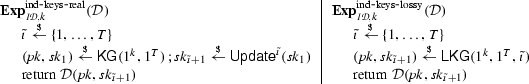
  $\mathcal {D}$ is said to $(t,\varepsilon )$-solve the key indistinguishability problem if it runs in time t and

  

  Furthermore, we say that is $(t,\varepsilon )$-key-indistinguishable, if no algorithm $(t,\varepsilon )$-solves the key-indistinguishability problem.

• 4. Lossiness. Let $\mathcal {I}_i$ be an impersonator for period i ($i \in \{1,\ldots ,T\}$), $st$ be its state. We consider the experiment played between $\mathcal {I}_i$ and a hypothetical challenger:

  

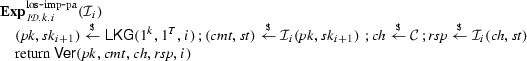
  The impersonator $\mathcal {I}_i$ is said to $\varepsilon$-solve the impersonation problem with respect to i-lossy public keys if . Furthermore, is said to be $\varepsilon$-lossy if, for any period $i \in \{1,\ldots ,T\}$, no (computationally unrestricted) algorithm $\varepsilon$-solves the impersonation problem with respect to i-lossy keys.

In addition, the commitment space of has min-entropy at least $\beta$, if for every period i, every security parameter $k$, and all honestly generated keys $( pk , sk _1) {\mathop {\leftarrow }\limits ^{{\scriptscriptstyle \$}}}{\mathsf {KG}}(1^ k )$, every bit string $cmt ^*$, if $sk _i = {\mathsf {Update}}^{i-1}( sk _1)$, then:

$$\begin{aligned} \left| {\Pr }\left[ \, cmt = cmt ^* \mid ( cmt , st ) {\mathop {\leftarrow }\limits ^{{\scriptscriptstyle \$}}}{\mathsf {Prove}}( sk _i)\,\right] \right| \le 2^{-\beta }. \end{aligned}$$

Usually, an identification scheme is also required to be sound, i.e., for a period i chosen uniformly at random, it should not be possible for an adversary to run the protocol with a honest verifier and to make the latter accept, if the public key has been generated honestly ($( pk , sk _1) {\mathop {\leftarrow }\limits ^{{\scriptscriptstyle \$}}}{\mathsf {KG}}(1^ k , 1^T)$) and if the adversary is only given a secret key $sk _{i+1}$. But, in our case, this soundness property follows directly from the key indistinguishability and the lossiness properties.

We could also consider more general lossy identification schemes where the simulatability of transcripts is computational instead of being statistical. However, we opted for not doing so because our security reduction is not tight with respect to the simulatability of transcripts.

We remark that, for $T=1$, a key-evolving lossy identification scheme becomes a standard lossy identification scheme, described in [5, 6].⁷

Finally, we say that is response-unique if the following holds either for every lossy public key or for every normal public key (or for both): for all periods $i \in \{1,\ldots ,T\}$, for all bit strings $cmt$ (which may or may not be a correctly generated commitment), and for all challenges $ch$, there exists at most one response $rsp$ such that ${\mathsf {Ver}}( pk , cmt , ch , rsp ,i)=1$.

3.2 Generalized Fiat–Shamir Transform

The forward-secure signature schemes considered in this paper are built from a key-evolving identification scheme via a straightforward generalization of the Fiat–Shamir transform [28], depicted in Fig. 2. More precisely, the signature for period i is just the signature obtained from a Fiat–Shamir transform with secret key $sk _i = {\mathsf {Update}}^{i-1}( sk _1)$ (with the period i included in the random oracle input).

Fig. 2

Generalized Fiat–Shamir transform for forward-secure signature

Let be the signature scheme obtained via this generalized Fiat–Shamir transform.

Main security theorem. The following theorem is a generalization of Theorem 1 in [5, 6] to key-evolving schemes. If we set $T=1$ in Theorem 3.1, we get the latter theorem with slightly improved bounds, since forward security for $T=1$ reduces to the notion of strong unforgeability for signature schemes. For the sake of simplicity and contrary to [5, 6] where the completeness property of the underlying lossy identification scheme was only assumed to hold statistically, we assume perfect completeness, as this is satisfied by all of the schemes that we consider.

Theorem 3.1

Let be a key-evolving lossy identification scheme whose commitment space has min-entropy at least $\beta$ (for every period i), let ${\mathsf {H}}$ be a hash function modeled as a random oracle, and let be the signature scheme obtained via the generalized Fiat–Shamir transform (Fig. 2). If is $\varepsilon _{s}$-simulatable, complete, $(t',\varepsilon ')$-key-indistinguishable, and $\varepsilon _{\ell }$-lossy, then is $(t,q_h,q_s,\varepsilon )$ existentially forward-secure in the random oracle model for:

$$\begin{aligned} \varepsilon&= T \, \left( \varepsilon ' + (q_h + 1) \varepsilon _\ell \right) + q_s \varepsilon _s + (q_h + q_s + 1) q_s / 2^\beta \quad \text { and }\\ t&\approx t' - (q_s \, t_{\mathsf {Sim-Sign}}+ (T-1) \, t_{\mathsf {Update}}) \end{aligned}$$

where $t_{{\mathsf {Sim-Sign}}}$ denotes the time to simulate a transcript using and $t_{\mathsf {Update}}$ denotes the time to update a secret key using ${\mathsf {Update}}$. Furthermore, if is response-unique, is also $(t,q_h,q_s,\varepsilon )$-forward-secure.

The proof of Theorem 3.1 is an adaptation of the proof in [5, 6] to the forward-security setting. As in [5, 6], the main idea of the proof is to switch the public key of the signature scheme with a lossy one, for which forgeries are information theoretically impossible with high probability. In our case, however, we need to guess the period $i^*$ of the signature output by the adversary, in order to choose the correct type of lossy key to be used in the reduction and this is why we lose a factor T in the reduction. Moreover, as in [5, 6], signatures queries are easy to answer thanks to the simulatability of the identification scheme. Finally, similarly to [5, 6] and contrary to [1], we remark that the factor $q_H$ only multiplies terms which are statistically negligible and, hence, it has no effect on the tightness of the proof.

Proof

Let us suppose there exists an adversary $\mathcal {A}$ which $(t,q_h,q_s,\varepsilon )$-breaks the existential forward security of . Let us consider the games $\text {G}_0, \ldots , \text {G}_9$ of Figs. 3 and 4. The random oracle $\mathbf{H }$ is simulated using a table $\mathsf {HT}$ containing all the previous queries to the oracle and its responses.

Before describing precisely all the games and formally showing that two consecutive games are indistinguishable, let us give a high-level overview of these games. The first game $\text {G}_0$ corresponds to the original security notion. We then change the way signatures are computed: instead of getting the challenge $ch$ from the random oracle after generating the commitment $cmt$, we first choose it and then program the random oracle. We deal with programming and the possible collisions that it could generate in the games $\text {G}_1$, $\text {G}_2$, and $\text {G}_3$. We then simulate all signatures using the transcript simulator in the game $\text {G}_4$, as $ch$ can now be chosen independently of $cmt$. From this point on, the secret keys are only used to answer the $\mathbf{Break }\hbox {-}\mathbf{In }$ queries. Hence, we can now guess the time period $i^*$ of the forgery, abort if this is not guessed correctly, and generate a lossy public key for period $i^*+1$ onwards (in the games $\text {G}_6$, $\text {G}_7$, and $\text {G}_8$). This makes us lose a factor T in the reduction. Finally, the lossiness property ensures that the adversary cannot generate a valid signature with non-negligible probability.

Let us now provide the proof details. First, we will assume that the set of queries to the random oracle made by the adversary always contains the query ${( cmt ^*, M ^*)}$. This is without loss of generality because, given any adversary, we can always create an adversary (with the same success probability and approximately the same running time) that performs this query before calling ${\mathbf{Finalize }}$. It only increases the total amount of hash queries by 1.

Fig. 3

Games $\text {G}_0,\ldots ,\text {G}_4$ for proof of Theorem 3.1. $\text {G}_1$ includes the boxed code at line 034 but $\text {G}_0$ does not

Fig. 4

Games $\text {G}_5,\ldots ,\text {G}_9$ for proof of Theorem 3.1. $\text {G}_6$ includes the boxed code at lines 525 and 556 but $\text {G}_5$ does not; $\text {G}_9$ includes the boxed code at line 757 but $\text {G}_7$ and $\text {G}_8$ do not

$\text {G}_0$ corresponds to a slightly stronger game than the game defining the existential forward security of a key-evolving signature built from a key-evolving scheme via generalized Fiat–Shamir transform. We only force the forgery to be such that ${( cmt ^*, M ^*, i^*)}$ is different from all the previous queries to the signing oracle, instead of just ${(M^*, i^*)}$ being different from all the previous queries. This corresponds to a security notion stronger than existential forward-security but still weaker than strong forward-security (where we have to consider ${( cmt ^*, rsp ^*, M ^*, i^*)}$).

In $\text {G}_0$, we have inlined the code of the random oracle in the procedure ${\mathsf {Sign}}$, and we set $\mathsf {bad}$ whenever $\mathbf{H }({( cmt , M ,i)})$ is already defined. We have also modified the code of the random oracle $\mathbf{H }$ such that the $\mathrm {fp}$-th query (the critical query eventually related to the forgery) is answered by $ch ^*$, a random challenge chosen in ${\mathbf{Initialize }}$, where $\mathrm {fp}$ is a random integer in the range $\{1, \ldots , q_h+1\}$. These modifications do not change the output of the original game.

To compute the probability ${\Pr \left[ \,{\text {G}_0(\mathcal {A}) \text{ sets } \mathsf {bad}}\,\right] }$, we remark that, for each signing query, the probability that there is a collision (i.e., $\mathsf {bad}$ is set for this query) is at most $(q_h + q_s + 1)/2^\beta$. By the union bound, we have ${\Pr \left[ \,{\text {G}_0(\mathcal {A}) \text{ sets } \mathsf {bad}}\,\right] } \le (q_h + q_s + 1) q_s /2^\beta$.

In $\text {G}_1$, when $\mathsf {bad}$ is set, a new random value for $\mathbf{H }({( cmt , M ,i)})$ is set in $\mathbf{Sign }$. Since $\text {G}_0$ and $\text {G}_1$ are identical until $\mathsf {bad}$, thanks to Lemma 2.1, we have ${\Pr \left[ \,{\text {G}_0(\mathcal {A}) \,{\Rightarrow }\,1}\,\right] } - {\Pr \left[ \,{\text {G}_1(\mathcal {A}) \,{\Rightarrow }\,1}\,\right] } \le {\Pr \left[ \,{\text {G}_0(\mathcal {A}) \text{ sets } \mathsf {bad}}\,\right] } \le (q_s + 1) q_s /2^\beta$.

In $\text {G}_2$, $\mathsf {bad}$ is no more set and the procedure $\mathbf{Sign }$ is rewritten in an equivalent way. Since the latter does not change the output of the game, we have ${\Pr \left[ \,{\text {G}_1(\mathcal {A}) \,{\Rightarrow }\,1}\,\right] } = {\Pr \left[ \,{\text {G}_2(\mathcal {A}) \,{\Rightarrow }\,1}\,\right] }$.

In $\text {G}_3$, the procedure $\mathbf{Sign }$ is changed such that the values $( cmt , ch , rsp )$ are computed using the transcript generation function . Since the latter does not change the output of the game, we have ${\Pr \left[ \,{\text {G}_2(\mathcal {A}) \,{\Rightarrow }\,1}\,\right] } = {\Pr \left[ \,{\text {G}_3(\mathcal {A}) \,{\Rightarrow }\,1}\,\right] }$.

In $\text {G}_4$, the $q_s$ calls to the transcript generation function are replaced by $q_s$ calls to the simulated transcript generation function . Since the statistical distance between the distributions output by and by is at most $\varepsilon _s$, we have ${\Pr \left[ \,{\text {G}_3(\mathcal {A}) \,{\Rightarrow }\,1}\,\right] } - {\Pr \left[ \,{\text {G}_4(\mathcal {A}) \,{\Rightarrow }\,1}\,\right] } \le q_s \varepsilon _s$.

In $\text {G}_5$, a period ${\tilde{\imath }}\in \{1, \ldots , T\}$ is chosen uniformly at random, and $\mathsf {bad}$ is set when the adversary queries $\mathbf{Break }\hbox {-}\mathbf{In }$ with a period $\mathrm {b}\le {\tilde{\imath }}$ or when the adversary outputs a signature for a period $i^* \ne {\tilde{\imath }}$. Since if $\text {G}_5$ outputs 1, we have $i^* < \mathrm {b}$, “$\mathsf {bad}$ is never set and $\text {G}_5$ outputs 1” (event $\text {G}_5(\mathcal {A}) \,{\Rightarrow }\,1 \wedge \mathsf {Good}_5$) if and only if “$i^* = {\tilde{\imath }}$ and $\text {G}_5$ outputs 1.” Therefore, we have:

$$\begin{aligned} {\Pr \left[ \,{\text {G}_5(\mathcal {A}) \,{\Rightarrow }\,1 \wedge \mathsf {Good}_5}\,\right] }&= \sum _{i=1}^T {\Pr \left[ \,{\text {G}_5(\mathcal {A}) \,{\Rightarrow }\,1 \wedge i^* = i = {\tilde{\imath }}}\,\right] } \\&= \frac{1}{T} {\Pr \left[ \,{\text {G}_5(\mathcal {A}) \,{\Rightarrow }\,1}\,\right] } = \frac{1}{T} {\Pr \left[ \,{\text {G}_4(\mathcal {A}) \,{\Rightarrow }\,1}\,\right] }, \end{aligned}$$

where the second equality comes from the fact that ${\Pr \left[ \,{{\tilde{\imath }}= i}\,\right] } = \frac{1}{T}$ and that the event “${\tilde{\imath }}= i$” is independent from the event “$\text {G}_5(\mathcal {A}) \,{\Rightarrow }\,1 \wedge i^* = i$.”

In $\text {G}_6$, the empty string $\bot$ is returned if $\mathbf{Break }\hbox {-}\mathbf{In }$ is queried with a period $i \le {\tilde{\imath }}$, and the game outputs 0 if $i^* \ne {\tilde{\imath }}$. Since $\text {G}_5$ and $\text {G}_6$ are identical until bad, according to Lemma 2.2, we have

$$\begin{aligned} {\Pr \left[ \,{\text {G}_5(\mathcal {A}) \,{\Rightarrow }\,1 \wedge \mathsf {Good}_5}\,\right] } = {\Pr \left[ \,{\text {G}_6(\mathcal {A}) \,{\Rightarrow }\,1 \wedge \mathsf {Good}_6}\,\right] } = {\Pr \left[ \,{\text {G}_6(\mathcal {A}) \,{\Rightarrow }\,1}\,\right] }. \end{aligned}$$

In $\text {G}_7$, some procedures have been rewritten in an equivalent way, and $\mathsf {bad}$ is now set when the query $( cmt ^*, M ^*)$ is not the $\mathrm {fp}^{\text {th}}$ query to the random oracle. Since the latter does not change the output of the experiment, we have ${\Pr \left[ \,{\text {G}_6(\mathcal {A}) \,{\Rightarrow }\,1}\,\right] } = {\Pr \left[ \,{\text {G}_7(\mathcal {A}) \,{\Rightarrow }\,1}\,\right] }$.

In $\text {G}_8$, the key is generated using the lossy key generation algorithm ${\mathsf {LKG}}$ for period ${\tilde{\imath }}$ instead of the normal key generation algorithm ${\mathsf {KG}}$. From any adversary $\mathcal {A}$ able to distinguish $\text {G}_7$ from $\text {G}_8$, it is straightforward to construct an adversary which $(t', \varepsilon '')$-solves the key indistinguishability problem with $t' \approx t + (q_s t_{\mathsf {Sim-Sign}}+ (T-1) t_{\mathsf {Update}})$ and $\varepsilon '' = \left| {\Pr \left[ \,{\text {G}_7(\mathcal {A}) \,{\Rightarrow }\,1}\,\right] } - {\Pr \left[ \,{\text {G}_8(\mathcal {A}) \,{\Rightarrow }\,1}\,\right] } \right|$. Therefore, thanks to the $(t',\varepsilon ')$-key-indistinguishability of , if the adversary runs in time approximately at most $t' - (q_s t_{\mathsf {Sim-Sign}}+ (T-1) t_{\mathsf {Update}})$:

$$\begin{aligned} {\Pr \left[ \,{\text {G}_7(\mathcal {A}) \,{\Rightarrow }\,1}\,\right] } - {\Pr \left[ \,{\text {G}_8(\mathcal {A}) \,{\Rightarrow }\,1}\,\right] } \le \varepsilon '. \end{aligned}$$

(3.1)

In $\text {G}_9$, the game outputs 0 if the signature does not correspond to the challenge $ch ^*$. Since we have

$$\begin{aligned} {\Pr \left[ \,{\text {G}_8(\mathcal {A}) \,{\Rightarrow }\,1 \wedge \mathsf {Good}_8}\,\right] }= & {} {\Pr \left[ \,{\text {G}_8(\mathcal {A}) \,{\Rightarrow }\,1}\,\right] } \cdot {\Pr \left[ \,{\mathsf {QT}[\mathrm {fp}] = ( cmt ^*, M ^*)}\,\right] } \\= & {} \frac{1}{q_h + 1} {\Pr \left[ \,{\text {G}_8(\mathcal {A}) \,{\Rightarrow }\,1}\,\right] }, \end{aligned}$$

and ${\Pr \left[ \,{\text {G}_9(\mathcal {A}) \,{\Rightarrow }\,1 \wedge \mathsf {Good}_9}\,\right] } = {\Pr \left[ \,{\text {G}_9(\mathcal {A}) \,{\Rightarrow }\,1}\,\right] }$, according to Lemma 2.2, we have ${\Pr \left[ \,{\text {G}_8(\mathcal {A}) \,{\Rightarrow }\,1}\,\right] } = (q_h + 1) {\Pr \left[ \,{\text {G}_9(\mathcal {A}) \,{\Rightarrow }\,1}\,\right] }$.

From any adversary $\mathcal {A}$ for $\text {G}_9$, it is straightforward to construct an adversary $\mathcal {I}$ (not necessarily computationally bounded) which $\varepsilon ''$-solves the impersonation problem with $\varepsilon '' = {\Pr \left[ \,{\text {G}_9(\mathcal {A}) \,{\Rightarrow }\,1}\,\right] }$. Therefore, we have ${\Pr \left[ \,{\text {G}_9(\mathcal {A}) \,{\Rightarrow }\,1}\,\right] } \le \varepsilon _\ell$.

From the previous equalities and inequalities, we deduce that, for any adversary $\mathcal {A}$ running in time approximately at most $t' - (q_s t_{\mathsf {Sim-Sign}}+ (T-1) t_{\mathsf {Update}})$:

$$\begin{aligned} \varepsilon \le {\Pr \left[ \,{\text {G}_0(\mathcal {A})}\,\right] } \le T \, \left( \varepsilon ' + (q_h + 1) \varepsilon _\ell \right) + q_s \varepsilon _s + (q_h + q_s + 1) q_s / 2^\beta . \end{aligned}$$

Let us now prove that is strongly forward-secure (with the same parameters) if is response-unique.

We first remark that, if we replace line 055 of $\text {G}_0$ in Fig. 3 by

$$\begin{aligned} {{\mathrm {if}}\ }~ S[{( cmt ^*, M ^*,i^*)}] = rsp ^*~ {{\mathrm {then}}\ }\end{aligned}$$

then we get exactly the game for forward security.

Therefore, if normal keys are response-unique, it is clear that this new game is equivalent to the original game $\text {G}_0$, since if $S[{( cmt ^*, M ^*,i^*)}]$ is defined, it is the only possible response $rsp ^*$.

If lossy keys are response-unique, to prove forward security, it is sufficient to replace lines 055, 558, and 758 for games $\text {G}_0,\ldots ,\text {G}_9$ in Figs. 3 and 4 by

$$\begin{aligned} {{\mathrm {if}}\ }~S[{( cmt ^*, M ^*,i^*)}] = rsp ^*~{{\mathrm {then}}\ }\end{aligned}$$

Then the probability the adversary wins the new game $\text {G}_9$ is still bounded by $\varepsilon _l$ since if $S[{( cmt ^*, M ^*,i^*)}]$ is defined, it is the only possible response $rsp ^*$. $\square$

Remark 3.2

As in the standard Fiat–Shamir transform, the signature obtained via the generalized transform consists of a commitment-response pair. However, in all schemes proposed in this paper, the commitment can be recovered from the challenge and the response. Hence, since the challenge is often shorter than the commitment, it is generally better to use the challenge-response pair as the signature in our schemes. Obviously, this change does not affect the security of our schemes.

Security theorems for comparisons with previous schemes. In the sequel, to be able to do a fair comparison, we also need the following variant of Theorem 3.1 and its associated straightforward corollary.

Theorem 3.3

Let be a key-evolving lossy identification scheme whose commitment space has min-entropy at least $\beta$ (for every period i), let ${\mathsf {H}}$ be a hash function modeled as a random oracle, and let be the signature scheme obtained via the generalized Fiat–Shamir transform. If -simulatable, complete, $(t',\varepsilon ')$-key-indistinguishable, and $\varepsilon _{\ell }$-lossy, then is $(t,q_h,q_s,\varepsilon ,\delta )$-selectively existentially forward-secure in the random oracle model for:

$$\begin{aligned} t \approx \left( t' - (T-1) \, t_{\mathsf {Update}}\right) \cdot \left( \varepsilon - q_s \varepsilon _s - (q_h + q_s + 1) q_s / 2^\beta \right) - q_s t_{\mathsf {Sim-Sign}}\end{aligned}$$

as long as

$$\begin{aligned} \varepsilon> & {} q_s \varepsilon _s + (q_h + q_s + 1) q_s/2^\beta \quad \text { and }\quad \\ \varepsilon '\le & {} \delta \, \left( 1 - \frac{1}{{\mathrm e}} \right) - \frac{(q_h + 1) \, \varepsilon _\ell }{\varepsilon - q_s \varepsilon _s - (q_h + q_s + 1) q_s / 2^\beta } \end{aligned}$$

where $t_{{\mathsf {Sim-Sign}}}$ denotes the time to simulate a transcript using , $t_{\mathsf {Update}}$ denotes the time to update a secret key using ${\mathsf {Update}}$, and ${\mathrm e}$ (not to be confused with e) is the base of the natural logarithm. Furthermore, if is response-unique, is also $(t,q_h,q_s,\varepsilon ,\delta )$-selectively forward-secure.

Corollary 3.4

Under the same hypothesis of Theorem 3.3, is $(t,q_h,q_s,\varepsilon ,\delta )$-selectively existentially forward-secure in the random oracle model for:

$$\begin{aligned} t \approx \frac{\left( t' - (T-1) \, t_{\mathsf {Update}}\right) \cdot \varepsilon }{2} - q_s t_{\mathsf {Sim-Sign}}\end{aligned}$$

as long as

$$\begin{aligned} \varepsilon \ge 2 \left( q_s \varepsilon _s + (q_h + q_s + 1) q_s / 2^\beta \right) \quad \text { and }\quad \varepsilon ' \le \delta \, \left( 1 - \frac{1}{{\mathrm e}} \right) - \frac{2 \, (q_h + 1) \, \varepsilon _\ell }{\varepsilon }. \end{aligned}$$

Furthermore, if  is response-unique, is also $(t,q_h,q_s,\varepsilon ,\delta )$-selectively forward-secure.

In concrete instantiations in the sequel, we often omit $t_{\mathsf {Update}}$ and $t_{\mathsf {Sim-Sign}}$ as these values are small compared to $t'$, for any reasonable parameters. For any $\varepsilon > 0$ satisfying the above inequalities, under the assumption of Remark 2.4, we can say that the scheme is about $({\textstyle \frac{t' \varepsilon }{2}}, q_h, q_s, T \varepsilon )$-forward-secure (i.e., provide about $\log _2(t'/(2 T))$ bits of security), if the underlying identification scheme is (about) $(t',{(1 - 1/e)}/2)$-hard. In other words, the security reduction loses a factor about T.

Proof of Corollary 3.4 from Theorem 3.3

It is a direct corollary of Theorem 3.3. The condition $\varepsilon > 2 \left( q_s \varepsilon _s + (q_h + q_s + 1) q_s / 2^\beta \right)$ ensures that $\varepsilon - q_s \varepsilon _s - (q_h + q_s + 1) q_s / 2^\beta \ge \varepsilon / 2$. $\square$

Proof of Theorem 3.3

Let us suppose there exists an adversary $\mathcal {A}$ that $(t,q_h,q_s,\varepsilon ,\delta )$-breaks . In particular, $\mathcal {A}$$(t,q_h,q_s,\varepsilon \delta )$-breaks .

The proof of Theorem 3.3 is very similar to the proof of Theorem 3.1. We use the same games, except for ${\mathbf{Initialize }}$ and ${\mathbf{Finalize }}$ of games $\text {G}_1,\ldots ,\text {G}_5$ which are replaced by the ones of game $\text {G}_6$. Indeed, in the game of the selective security, a period ${\tilde{\imath }}$ is chosen in ${\mathbf{Initialize }}$ and the adversary has to forge a signature for this period. Then the proof is identical except that ${\Pr \left[ \,{\text {G}_4(\mathcal {A}) \,{\Rightarrow }\,1}\,\right] } = {\Pr \left[ \,{\text {G}_5(\mathcal {A}) \,{\Rightarrow }\,1}\,\right] } = {\Pr \left[ \,{\text {G}_6(\mathcal {A}) \,{\Rightarrow }\,1}\,\right] }$ and except for the inequality of Eq. (3.1) (p. 20).

We remark that, if we write $\gamma = \left( q_s \varepsilon _s + (q_h + q_s + 1) q_s / 2^\beta \right)$:

$$\begin{aligned} {\Pr \left[ \,{\text {G}_7(\mathcal {A}) \,{\Rightarrow }\,1}\,\right] }&\ge \varepsilon - \gamma \text { with probability at least } \delta \text { over } ( pk , sk _1,{\tilde{\imath }}) \end{aligned}$$

(3.2)

$$\begin{aligned} {\Pr \left[ \,{\text {G}_8(\mathcal {A}) \,{\Rightarrow }\,1}\,\right] }&\le (q_h + 1) \, \varepsilon _\ell \end{aligned}$$

(3.3)

Let us construct an adversary $\mathcal {B}$ which $(t'',\varepsilon '')$-breaks the key indistinguishability property with $t'' \approx \frac{t + q_s t_{\mathsf {Sim-Sign}}}{\varepsilon - \gamma } + (T-1) t_{\mathsf {Update}}$ and $\varepsilon '' \ge \delta \, \left( 1 - \frac{1}{{\mathrm e}} \right) - \frac{1}{\varepsilon - \gamma } \, (q_h + 1) \, \varepsilon _\ell$. $\mathcal {B}$ takes as input a period ${\tilde{\imath }}$, a public key $pk$ and a secret key $sk _{{\tilde{\imath }}+1}$ for period ${\tilde{\imath }}+1$. It then runs $\mathcal {A}$$\frac{1}{\varepsilon - \gamma }$ times and simulates the oracles as in game $\text {G}_7$ (or $\text {G}_8$, which is equivalent), except for ${\mathbf{Initialize }}$ where it uses directly its inputs ${\tilde{\imath }}$, $pk$ and $sk _{{\tilde{\imath }}+1}$ (instead of picking them at random). If $\mathcal {A}$ outputs a correct forgery during one of its runs, $\mathcal {B}$ outputs 1. Otherwise, it outputs 0.

Clearly $\mathcal {B}$ perfectly simulates the environment of $\mathcal {A}$ in the game $\text {G}_7$, if $pk$ is not lossy, or in the game $\text {G}_8$, if $pk$ is lossy. According to Eq. (3.2), if $pk$ is not lossy, we have

$$\begin{aligned} {\Pr }\left[ \,\mathcal {B}\,{\Rightarrow }\,1 \mid pk \text { normal}\,\right]&\ge \, \delta \, {\Pr }\left[ \,\mathcal {B}\,{\Rightarrow }\,1 \Bigg |\begin{array}{c} pk \hbox { normal and }\\ {\Pr \left[ \,{\text {G}_7(\mathcal {A}) \,{\Rightarrow }\,1}\,\right] }\\ \ge \varepsilon -\gamma \\ \end{array}\,\right] \\&\ge \, \delta \, \left( 1 - {\left( 1 - (\varepsilon - \gamma ) \right) }^{\frac{1}{\varepsilon - \gamma }} \right) \,\ge \, \delta \, \left( 1 - \frac{1}{{\mathrm e}} \right) \end{aligned}$$

and, according to Eq. (3.3), if $pk$ is lossy, we have

$$\begin{aligned} {\Pr }\left[ \,\mathcal {B}\,{\Rightarrow }\,1 \mid pk \text { lossy}\,\right] \,\le \, \frac{1}{\varepsilon - \gamma } \, {\Pr \left[ \,{\text {G}_8(\mathcal {A}) \,{\Rightarrow }\,1}\,\right] } \,\le \, \frac{1}{\varepsilon - \gamma } \, (q_h + 1) \, \varepsilon _\ell . \end{aligned}$$

Therefore, the advantage of $\mathcal {B}$ is $\varepsilon '' \ge \delta \, \left( 1 - \frac{1}{{\mathrm e}} \right) - \frac{1}{\varepsilon - \gamma } \, (q_h+1) \, \varepsilon _\ell$. Its running time is $t'' \approx \frac{t + q_s t_{\mathsf {Sim-Sign}}}{\varepsilon - \gamma } + (T-1) t_{\mathsf {Update}}$. This proves the theorem. $\square$

4 Tighter Security Reductions for Guillou–Quisquater-Like Schemes

In this section, we prove tighter security reductions for the Guillou–Quisquater scheme (GQ [34]) and for a slight variant of the Itkis–Reyzin scheme (IR [41]), which can also be seen as a forward-secure extension of the GQ scheme. We analyze the practical performance of this new scheme in the next section of this article.

4.1 Guillou–Quisquater Scheme

Let us describe the identification scheme corresponding to the GQ signature scheme,⁸ before presenting our tight reduction and comparing it with the swap method.

Scheme. Let N be a product of two distinct ${\ell _N}$-bit primes $p_1,p_2$ and let e be a ${\ell _e}$-bit prime, co-prime to $\phi (N) = (p_1 - 1)(p_2 - 1)$, chosen uniformly at random.⁹ Let S be an element chosen uniformly at random in ${{\mathbb Z}}_N^*$ and let $U = S^e \bmod N$. Let $\mathfrak {c}= e \ge 2^{{\ell _e}-1}$ and $\mathcal {C}= \{0,\ldots ,\mathfrak {c}-1\}$. The (normal) public key is $pk = (N,e,U)$ and the secret key is $sk =(N,e,S)$.

The goal of the identification scheme is to implicitly prove U is an e-residue.¹⁰ The identification scheme is depicted in Figs. 5 and 6. It works as follows. We recall that the scheme only supports one time-period (i.e., $T=1$). Therefore, the ${\mathsf {Update}}$ algorithm is not needed and $sk _1= sk$. First, the prover chooses a random element $R \in {{\mathbb Z}}_N^*$, computes $Y \leftarrow R^e \bmod N$. It sends Y to the verifier, which in turn chooses $c \in \{0,\ldots ,\mathfrak {c}-1\}$ and returns it to the prover. Upon receiving $c$, the prover computes $Z \leftarrow R \cdot S^ c \bmod N$ and sends this value to the verifier. Finally, the verifier checks whether $Z \in {{\mathbb Z}}_N^*$ and $Z^e = Y \cdot U^ c$ and accepts only in this case.¹¹

The algorithm ${\mathsf {LKG}}$ chooses e and $N=p_1p_2$ such that e divides $p_1-1$, instead of being co-prime to $\phi (N)$, and chooses U uniformly at random among the non-e-residue modulo N. The lossy public key is then $pk = (N,e,U)$. Propositions B.13 and B.16 show that if U is chosen uniformly at random in ${{\mathbb Z}}_N^*$, it is not an e-residue with probability $1-1/e$ and that it is possible to efficiently check whether U is an e-residue or not if the factorization of N is known: U is a e-residue if and only if, for any $j \in \{1,2\}$, e does not divide $p_j-1$ or $U^{(p_j - 1) / e} = 1\bmod p_j$.

Fig. 5

Formal description of the Guillou–Quisquater identification scheme (${\ell _e}$ and ${\ell _N}$ are two parameters depending on $k$ and $\mathfrak {c}= e \ge 2^{{\ell _e}-1}$)

Fig. 6

Pictorial description of the Guillou–Quisquater identification scheme

In the original scheme, any prime number e of large enough length ${\ell _e}$ could be used—to get negligible soundness or lossiness probability, ${\ell _e}$ needs to be at least equal to $k$. However, for our proof to work, we need the $\phi$-hiding assumption to hold. This implies in addition that ${\ell _e}< {\ell _N}/ 4$.

Security. Existing proofs for the GQ scheme lose a factor $q_h$ in the reduction. In this section, we prove the previously described identification scheme is a lossy identification scheme, under the $\phi$-hiding assumption. This yields a security proof of the strong unforgeability of the GQ scheme, with a tight reduction to this assumption.

More formally, we prove the following theorem:

Theorem 4.1

The identification scheme depicted in Figs. 5 and 6 is complete, perfectly simulatable, key-indistinguishable, $(1/\mathfrak {c})$-lossy, and response-unique. More precisely, if the $\phi$-hiding problem is $(t',\varepsilon ')$-hard, then the identification scheme is $(t,\varepsilon )$-key-indistinguishable for:

$$\begin{aligned} t \approx t' \quad \text { and }\quad \varepsilon \le \varepsilon ' + \frac{1}{2^{{\ell _e}-1}}. \end{aligned}$$

Furthermore, the min-entropy $\beta$ of the commitment space is $\log _2(\phi (N)) \ge {\ell _N}-1$.

Thanks to Corollary 3.4 (with $T=1$), we have the following corollary:

Theorem 4.2

If the $\phi$-hiding problem is $(t',\varepsilon ')$-hard, then the GQ scheme is $(t,q_h,q_s,\varepsilon ,\delta )$-selectively forward-secure for $T=1$ period in the random oracle model for:

$$\begin{aligned} t \approx \frac{t' \cdot \varepsilon }{2} \end{aligned}$$

as long as

$$\begin{aligned} \varepsilon \ge 2 \frac{(q_h + q_s + 1) q_s}{2^{{\ell _N}- 1}} \quad \text { and }\quad \varepsilon ' + \frac{1}{2^{{\ell _e}-1}} \le \delta \left( 1 - \frac{1}{{\mathrm e}} \right) - \frac{2\, (q_h + 1)}{2^{{\ell _e}- 1} \, \varepsilon }, \end{aligned}$$

where ${\mathrm e}$ (not to be confused with e) is the base of the natural logarithm.

Under the assumption of Remark 2.4, we can say that the scheme is about $({\textstyle \frac{t \varepsilon }{2}}, q_h, q_s, \varepsilon )$-strongly-unforgeable if the $\phi$-hiding problem is $(t,(1 - 1/e)/2)$-hard. This means roughly that if we want a $k$-bit security, the modulus has to correspond to a security level of $k ' \approx k$ bits, which is tight.

Proof of Theorem 4.1

The proof that is complete follows immediately from the fact that, if $U = S^e \bmod N$, an honest execution of the protocol will always result in acceptance as $Z^e = {(R \cdot S^{ c })}^e = R^e \cdot {(S^e)}^{ c } = Y \cdot U^{ c }$.

Simulatability follows from the fact that, given $pk = (N,e, U)$, we can easily generate transcripts whose distribution is perfectly indistinguishable from the transcripts output by an honest execution of the protocol. This is done by choosing Z uniformly at random in ${{\mathbb Z}}^*_N$ and $c$ uniformly at random in $\{0,\ldots ,\mathfrak {c}-1\}$, and setting $Y = Z^e / U^{ c }$.

Let us prove the key indistinguishability property. When e is co-prime with $\phi (N)$, the function f defined by $f(x)=x^e \bmod N$ is a permutation over ${{\mathbb Z}}_N^*$ (see, e.g., Corollary B.14). Therefore, when $pk =(N,e,U) {\mathop {\leftarrow }\limits ^{{\scriptscriptstyle \$}}}{\mathsf {KG}}(1^ k ,1)$, the element $U = S^e \in {{\mathbb Z}}_N^*$ (with $S {\mathop {\leftarrow }\limits ^{{\scriptscriptstyle \$}}}{{\mathbb Z}}_N^*$) is uniformly random. The distribution of normal public keys is therefore indistinguishable from the one where e divides $\phi (N)$ and U is chosen uniformly at random, according to the $\phi$-hiding assumption. And in this latter distribution, U is not a e-residue with probability $\ge 1-1/e \ge 1-1/2^{{\ell _e}-1}$ according to Corollary B.15, so this distribution is $(1/2^{{\ell _e}-1})$-close to the distribution of lossy keys according to Lemma 2.3. Hence, we get the bound of the theorem.

To show that is lossy, we note that, when the public key is lossy, for every element Y chosen by the adversary, there exists only one value of $c \in \{0,\ldots ,\mathfrak {c}-1\}$ for which there exists a response Z that is considered valid by the verifier. To see why, assume for the sake of contradiction that there exist two different values $c _{1}$ and $c _{2}$ in $\{0,\ldots ,\mathfrak {c}-1\}$ for which there exists a valid response. Denote by $Z_{1}$ and $Z_{2}$ one of the valid responses in each case. Without loss of generality, assume that $c _{1} < c _{2}$. Since $Z_{1}^e = Y \cdot U^{ c _{1}}$ and $Z_{2}^e = Y \cdot U^{ c _{2}}$, we have that ${(Z_{2}/Z_{1})}^e = U^{ c _{2}- c _{1}}$. As $c _{2}- c _{1}$ is a positive number smaller than $2^{{\ell _e}-1}$, it is co-prime to e (since e is a prime and $e \ge 2^{{\ell _e}-1}$). Therefore, according to Bézout’s identity, there exists two integers u, v such that: $u e + v ( c _2- c _1) = 1$. So:

$$\begin{aligned} U = U^{u e + v ( c _2- c _1)} = {(U^u)}^e {(U^{ c _{2}- c _{1}})}^v = {\left( U^u {(Z_{2}/Z_{1})}^v\right) }^e \end{aligned}$$

and U is a e-residue, which is impossible. This means that the probability that a valid response $Z_i$ exists in the case where U is not a e-residue is at most $1/\mathfrak {c}$. It follows that is $1/\mathfrak {c}$-lossy.

Response-uniqueness of follows from the fact that for any normal public key $pk =(N,e,U)$, e is co-prime with $\phi (N)$ and so the function f defined by $f(x)=x^e \bmod N$ is a permutation over ${{\mathbb Z}}_N^*$. For a commitment Y and a challenge $c$, the only response that is accepted by the verifier is therefore: $Z = {(Y \cdot U^ c )}^{1/e}$. Note that since $Z \in {{\mathbb Z}}_N^{*}$ and $Z^e = Y \cdot U^ c$, Y is also necessarily in ${{\mathbb Z}}_N^*$.

Finally, as for any normal public key $pk =(N,e,U)$, the function f defined by $f(x)=x^e \bmod N$ is a permutation over ${{\mathbb Z}}_N^*$, commitments $R^e$ are uniformly random in ${{\mathbb Z}}_N^*$. Therefore the commitment space has min-entropy$\log _2(\phi (N)) \ge {\ell _N}-1$. $\square$

Comparison with the swap method. Applying the swap method [53] to the GQ identification scheme can also provide a signature with a tight reduction, to the RSA problem. But in this case, the signing algorithm needs to compute the e-root of the output of the random oracle modulo N. Therefore, instead of requiring two exponentiations modulo N with a ${\ell _e}$-bit exponent, the signing algorithm requires one such exponentiation and one exponentiation modulo N with a ${\ell _N}$-bit exponent. So, our signing algorithm is about ${\ell _N}/ (2{\ell _e})$ times faster, for the same parameters and the same security level, if we consider the $\phi$-hiding problem is as hard as the RSA problem, and if we disregard the small differences of the exact tightness of the reductions. Furthermore, the swap method cannot be directly extended to the forward-secure extension of the GQ scheme, described in the next section, because the prover has to know the factorization of N.

4.2 Variant of the Itkis–Reyzin Scheme

Scheme. The idea of this forward-secure extension of the GQ scheme consists in using a different e for each period. More precisely, let $e_1,\ldots ,e_T$ be T distinct ${\ell _e}$-bit primes chosen uniformly at random, among ${\ell _e}$-bit primes that are co-prime to $\phi (N)$. Let $f_i = e_{i+1}\cdots e_T$, $f_T = 1$, and $E = e_1 \dots e_T$. Let S be an element chosen uniformly at random in ${{\mathbb Z}}_N^*$ and let $U = S^E \bmod N$. Let $S_i = S^{E/e_i}$ and $S'_i = S^{E/f_i}$. Then the public key is $pk = (N,e_1,\ldots ,e_T,U)$ and the secret key for period i is $sk _i = (N,e_i,\ldots ,e_T,S_i,S'_i)$. We remark we can easily compute $sk _{i+1}$ from $sk _i$, since $S_{i+1} = {S'}_{i}^{f_{i+1}} \bmod N$ and ${S'}_{i+1} = {S'}_i^{e_{i+1}} \bmod N$.

For period i, we have $S_i^{e_i} = U$ and the identification scheme works exactly as the previous one with public key $pk =(N,e_i,U)$ and secret key $sk =(N,e_i,S_i)$.

For the sake of simplicity, in this naive description of the scheme, we store the exponents $e_1, \ldots , e_T$ in both the public and secret keys. Therefore, the keys are linear in T, the number of periods. It is possible to have constant-size keys, either by using fixed exponents,¹² or by computing the exponents using a random oracle. This will be discussed in Sect. 5.1.

Security. The security proof is similar to the one for the previous scheme, with the main difference being the description of the lossy key generation algorithm ${\mathsf {LKG}}$. More precisely, on input $(1^ k ,1^T, i)$, the algorithm ${\mathsf {LKG}}$ generates $e_i$ and $N=p_1 p_2$ such that $e_i$ divides $p_1-1$, instead of being co-prime to $\phi (N)$, and chooses $U'$ uniformly at random among the non-$e_i$-residues modulo N. Then it chooses $T-1$ distinct random ${\ell _e}{}$-bit primes $e_1,\ldots ,e_{i-1},e_{i+1},\ldots , e_{T}$, and sets $U = U'^{e_{i+1} \cdots e_T} \bmod N$, $S_{i+1} = U'^{e_{i+2}\cdots e_T} \bmod N$ and $S'_{i+1} = U'^{e_{i+1}} \bmod N$. The public key is $pk =(N,e_1,\ldots ,e_T,U)$ and the secret key for period $i+1$ is $sk _{i+1} = (N,e_{i+1},\ldots ,e_T,S_{i+1},S'_{i+1})$ (or $\perp$ if $i=T$). We remark that, since $U'$ is a non-$e_i$-residue, U is also a non-$e_i$-residue and so the public key $pk$ is i-lossy.

More formally, using a similar analysis as for Theorem 4.1, we can prove the following theorem.

Theorem 4.3

The identification scheme described above is complete, perfectly simulatable, key-indistinguishable, $(1/\mathfrak {c})$-lossy, and response-unique. More precisely, if the $\phi$-hiding problem is $(t',\varepsilon ')$-hard, then the identification scheme is $(t,\varepsilon )$-key-indistinguishable for:

$$\begin{aligned} t \approx t' \quad \text { and }\quad \varepsilon \le \varepsilon ' + \frac{1}{2^{{\ell _e}-1}}. \end{aligned}$$

Furthermore, the min-entropy $\beta$ of the commitment space is $\log _2(\phi (N)) \ge {\ell _N}-1$.

Theorem 4.4

If the $\phi$-hiding problem is $(t',\varepsilon ')$-hard, then our variant of the IR scheme is $(t,q_h,q_s,\varepsilon ,\delta )$-selectively forward-secure in the random oracle model for:

$$\begin{aligned} t \approx \frac{t' \cdot \varepsilon }{2} \end{aligned}$$

as long as

$$\begin{aligned} \varepsilon \ge 2 \frac{(q_h + q_s + 1) q_s}{2^{{\ell _N}- 1}} \quad \text { and }\quad \varepsilon ' + \frac{1}{2^{{\ell _e}-1}} \le \delta \left( 1 - \frac{1}{{\mathrm e}} \right) - \frac{2\, (q_h + 1)}{2^{{\ell _e}- 1} \, \varepsilon }, \end{aligned}$$

where ${\mathrm e}$ (not to be confused with e) is the base of the natural logarithm.

Under the assumption of Remark 2.4, we can say that the scheme is about $({\textstyle \frac{t \varepsilon }{2}}, q_h, q_s, T \varepsilon )$-forward-secure if the $\phi$-hiding problem is $(t,(1 - 1/e)/2)$-hard. This means roughly that if we want a $k$-bit security, the modulus has to correspond to a security level of $k ' \approx k + \log _2(T)$ bits ($k'$ being an approximate solution of $2^{ k '} = \frac{2^ k \varepsilon }{2} \frac{1}{T \varepsilon }$).

5 Analysis of our Variant of the Itkis–Reyzin Scheme

In this section, we analyze our variant of the IR scheme and compare it with the original IR scheme [41] and the MMM scheme [52].

5.1 Computation of the Exponents $e_1,\ldots ,e_T$

As explained before, storing the exponents $e_1,\ldots ,e_T$ in the keys is not a good idea since the key size becomes linear in T. Since we need $e_1,\ldots ,e_T$ to be random primes to be able to do the reduction of key indistinguishability property to the $\phi$-hiding assumption, we can use a second hash function ${\mathsf {H}}'$ (also modeled as a random oracle in the proof) that outputs prime numbers of length ${\ell _e}$, and set $e_i = {\mathsf {H}}'(i)$.

Hash function for prime numbers which can be modeled as a random oracle. We can construct a hash function ${\mathsf {H}}'$ that outputs prime numbers of length ${\ell _e}$, from a classical hash function ${\mathsf {H}}''$ that only outputs ${\ell _e}$-bit strings, as ${\mathsf {H}}'(i) = {\mathsf {AlgH}}'_{{\mathsf {H}}''}(i)$ where the algorithm ${\mathsf {AlgH}}'$ is depicted in Fig. 7. This construction is close to the construction of a pseudorandom function (PRF) mapping to prime numbers in [39].

Furthermore, we remark that, if ${\mathsf {H}}''$ is modeled as a random oracle, then so can ${\mathsf {H}}' = {\mathsf {AlgH}}'_{{\mathsf {H}}''}$. More precisely, we can simulate any experiment with a random oracle ${\mathsf {H}}'$ that outputs prime numbers, by an experiment with random oracle ${\mathsf {H}}''$, by setting ${\mathsf {H}}'' = {\mathsf {AlgProgH}}''_{{\mathsf {H}}'}$, where the algorithm ${\mathsf {AlgProgH}}''$ is depicted in Fig. 7. When the primality test ${\mathsf {isPrime}}$ is probabilistic (instead of being deterministic), the simulation might not be perfect but is still statistically indistinguishable.

Fig. 7

Construction of a hash function ${\mathsf {AlgH}}'_{{\mathsf {H}}''} = {\mathsf {H}}'$ which outputs prime numbers, from a classical hash function ${\mathsf {H}}''$ which outputs ${\ell _e}$-bit string; and algorithm ${\mathsf {AlgProgH}}''$ which can simulate ${\mathsf {H}}''$ in such a way that ${\mathsf {AlgH}}'_{{\mathsf {AlgProgH}}''_{{\mathsf {H}}'}} = {\mathsf {H}}'$. ${\mathsf {isPrime}}$ is a primality test. $\mathsf {HT}''$ is a table which is initially empty

For efficiency purposes, it is necessary to use a probabilistic primality test for ${\mathsf {isPrime}}$, such as Miller–Rabin. Let us now study the error probability of${\mathsf {AlgH}}'$. To do that, let C denote the random variable equal to the number of primality tests needed in ${\mathsf {AlgH}}'$ (i.e., the final value of $cpt + 1$), if the primality tests are deterministic. According to Proposition B.18, C is a geometric random variable of parameter at least $1 / ({\ell _e}-1)$. So its expectation ${{\mathbf {E}}\left[ \,{C}\,\right] }$, the average number of calls to ${\mathsf {isPrime}}$, is at most ${\ell _e}-1$. Let us suppose the error probability of the test (i.e., the probability a composite number is considered prime) is $\varepsilon _p = 2^{-\rho }$. In this case, the error probability of ${\mathsf {AlgH}}'$ for input i is at most

Let us now analyze the security of the resulting scheme when $e_i$ is set to ${\mathsf {AlgH}}'(i)$. We suppose that $sk _i$ contains the exponent $e_i$. The secret key length is increased only by a small amount and the signing algorithm becomes faster, since it does not need to recompute $e_i$. For the sake of simplicity, we suppose ${\mathsf {KG}}$, ${\mathsf {LKG}}$, and ${\mathsf {Update}}$ use a deterministic algorithm ${\mathsf {isPrime}}'$ instead of ${\mathsf {isPrime}}$ for the generation of the exponents $e_i = {\mathsf {AlgH}}'(i)$.¹³ In the resulting scheme, the only difference in the security proof for when the exponents $e_1,\ldots ,e_T$ are stored in the public key is the following: the call to ${\mathsf {Ver}}$ in the procedure ${\mathbf{Finalize }}$ might compute an exponent $e_{i^*} = {\mathsf {AlgH}}'(i^*)$ different from the one computed by ${\mathsf {LKG}}$. The use of a deterministic primality test for ${\mathsf {KG}}$, ${\mathsf {LKG}}$, and ${\mathsf {Update}}$ ensures that everywhere else is the security reduction, the exponents $e_i$ are computed correctly. We do not want to do such an assumption for the primality test for ${\mathsf {Ver}}$, as we want to optimize the speed of ${\mathsf {Ver}}$ as much as possible.

We can adapt the security proof by replacing ${\mathsf {isPrime}}$ in ${\mathsf {AlgH}}'$ in the verification in the procedure ${\mathbf{Finalize }}$ of the forward security game by a deterministic algorithm ${\mathsf {isPrime}}'$. This just adds a term $({\ell _e}- 1) \varepsilon _p$ to the final probability for the adversary to win the original game.

Let us now analyze the performance of${\mathsf {AlgH}}'$. If we forget the probability of errors of the primality test and do not take into account the time to call ${\mathsf {H}}''$,¹⁴ the average time of ${\mathsf {AlgH}}'$ is $({{\mathbf {E}}\left[ \,{C}\,\right] } - 1) t_{\mathsf {isPrime-composite}}+ t_{\mathsf {isPrime-prime}}$, where $t_{\mathsf {isPrime-composite}}$ is the average running time of ${\mathsf {isPrime}}$ if its input is a composite number, and $t_{\mathsf {isPrime-prime}}$ is the average running time of ${\mathsf {isPrime}}$ if its input is a prime.

For Miller–Rabin test, if the input is prime, the algorithm roughly does $\rho /2$ exponentiations modulo an ${\ell _e}$-bit number with an ${\ell _e}$-bit exponent. Otherwise, if the input is a composite number, it does fewer than 4 / 3 such exponentiations on average.¹⁵ Therefore, $t_{\mathsf {isPrime-prime}}\approx \rho {\textstyle \frac{3}{2}} \, \frac{1}{2} \, {\ell _e}^3$ and $t_{\mathsf {isPrime-composite}}\approx {\textstyle \frac{3}{2}} \, {\textstyle \frac{4}{3}} \, {\ell _e}^3$, therefore the total time is about $({\textstyle \frac{3}{4}} \rho + 2 {\ell _e}) {\ell _e}^3$.¹⁶ In comparison, the time of a signature or a verification (if the exponents $e_1,\ldots ,e_T$ are stored in the public key) is the time of two exponentiations with a modulus of length ${\ell _N}$ and an exponent of length ${\ell _e}$, that means about $2 {\ell _N} k ^2$. A practical comparison can be found in Table 2.

5.2 Optimizations

In this section, we analyze optimizations of the original IR scheme and see that they can be applied to our scheme too. We also propose a specific optimization for our scheme.

Checking$Z \ne 0 \bmod N$instead of$Z \in {{\mathbb Z}}_N^*$in${\mathsf {Ver}}$. As explained in Footnote 11, we can change the test $Z \in {{\mathbb Z}}_N^*$ in ${\mathsf {Ver}}$ by the test $Z \ne 0 \bmod N$. We suppose that this optimization is done in our comparison in Table 2.

$e_i$power of small primes. If we slightly change the $e_i$ to be power of small primes $\varepsilon _i$: $e_i = \varepsilon _i^{{\ell _e}/\lfloor \log (\varepsilon _i)\rfloor }$, we can make the generation of $e_i$ faster since generating a small ${\ell _e}'$-bit prime $\varepsilon _i$ is about ${({\ell _e}/{\ell _e}')}^3$ faster than generating a ${\ell _e}$-bit prime $e_i$. However, we need to change the $\phi$-hiding assumption in order to be able to do the security reduction.¹⁷ We remark that all the proofs remain the same when $e_i$ is a power of a (small) prime instead of a prime. In particular, the following fact does not depend on whether e is a prime or not: all elements in ${{\mathbb Z}}_N^*$ are e-residues when e is co-prime with $\phi (N)$, while at most 1 / e of them are e-residues when e divides $\phi (N)$ (see Corollaries B.14 and B.15).

Pebbling. We also remark that the pebbling mechanism described in [41] can directly be applied to our scheme.

Storing$cpt$. Another possible trade-off consists in storing the last $cpt$ of ${\mathsf {AlgH}}'$ for each i, in the public and secret keys. Since ${{\mathbf {E}}\left[ \,{C}\,\right] } \le {\ell _e}-1$, the expected size of $cpt$ is $\log _2{{\ell _e}}$ and storing them increases the size of the keys by $T \log _2{{\ell _e}}$. For small values of T this can be useful, since this completely removes the necessity of ${\mathsf {isPrime}}$ in ${\mathsf {Sign}}$, ${\mathsf {Ver}}$, and ${\mathsf {Update}}$.

5.3 Choice of Parameters

In order to be able to compare the original IR scheme with our scheme, we need to choose various parameters. In Table 1, we show our choice of parameters for two security levels: $k = 80$ bits and $k = 128$ bits. When choosing these parameters, we considered a value of $T=2^{20}$, as it enables to update the key every hour for up to 120 years. In both cases, $\varepsilon _p = 2^{-\rho }$ denotes the maximum error probability of the probabilistic primality test used in the random oracle for prime numbers ${\mathsf {H}}'$, whereas $q_h$ and $q_s$ specify the maximum number of queries to the random oracle and to the signing oracle, respectively, in the forward-security game. Choices of $q_h$ and $q_s$ comes from [53]: $q_h = 2^ k$ because hash queries can be computed by the adversary itself, while $q_s$ is much lower as each signing query needs to be answered by an honest user.

Let us explain our choice for ${\ell _e}$. As in [53], we suppose $T\varepsilon ,\delta \ge 2^{-20} \approx 10^{-6}$.¹⁸ And we chose ${\ell _e}\approx k + 43$ to satisfy inequalities in security reductions in Theorem 4.4 and Theorem 5.1.¹⁹ In the sequel, all the parameters are fixed except the length ${\ell _N}$ of the modulus.

Table 1 Choice of parameters

5.4 Comparison with Existing Schemes

Comparison with the Itkis-Reyzin scheme. In this section, we compare the original IR scheme without optimization with our scheme (in which $e_i$ is stored in the secret key $sk _i$, as in the IR scheme). The original IR scheme is very close to our scheme. The only differences are that the IR scheme requires that the factors $p_1$ and $p_2$ of the modulus N are safe primes²⁰ and that IR signatures for period i contain the used exponent $e_i$. Therefore the IR verification algorithm does not need to recompute the exponent, and is faster. In order to prevent an adversary from using an exponent for the break-in period to sign messages for an older period, the exponent has to be in a different set for each period. The security of the scheme comes from the strong RSA assumption. Unfortunately, we cannot use such an optimization with our security reduction for our scheme, because we need to know which exponent the adversary will use to make the key lossy for this exponent. But, as explained in Sect. 5.2, the other optimizations of the original IR scheme can also be applied to our scheme.

We first remark that for the same parameters $k ,{\ell _e},{\ell _N}$, our key generation algorithm is slightly faster since it does not require safe primes; and our signing and key update algorithms are as fast as the IR ones. The key and signature lengths of the signatures are nearly the same as the IR ones. (IR signatures are only ${\ell _e}$-bits longer than our signatures.) The real difference is the verification time since our verification algorithm needs to recompute the $e_i$, contrary to the IR scheme. Verification consists of two exponentiations (modulo N with an ${\ell _e}$-bit exponent) for the original scheme and two exponentiations and an evaluation of the random prime oracle (roughly equivalent to a random prime generation) for our scheme.

Let us now focus on the exact security of the two schemes. As explained by Kakvi and Kiltz in [44], the best known attacks against the $\phi$-hiding problems are the factorization of N. Let us also consider it is true for the strong RSA problem (since it just strengthens our result if it is not the case). We recall that currently, no reductions are known between the strong RSA and the $\phi$-hiding problems.

In Appendix C.3, we show the following theorem, for the Itkis–Reyzin scheme:

Theorem 5.1

If the strong-RSA problem is $(t',\varepsilon ')$-hard, then the previous scheme is $(t, q_h, q_s, \varepsilon , \delta )$-selectively forward-secure in the random oracle model for:

$$\begin{aligned} t \approx \frac{t' \cdot \varepsilon }{4 q_h + 6} \end{aligned}$$

as long as

$$\begin{aligned} \varepsilon \ge 2 \left( \frac{(q_h + q_s + 1) q_s}{2^{{\ell _N}-2{\ell _e}-2}} + \frac{q_h + 1}{2^{{\ell _e}- 1}} \right) \quad \text { and }\quad \varepsilon ' \le \delta {\left( 1 - \frac{1}{{\mathrm e}} \right) }^2, \end{aligned}$$

where ${\mathrm e}$ (not to be confused with e) is the base of the natural logarithm.

For any $\varepsilon > 0$ satisfying the above inequalities, under the assumption of Remark 2.4, we can say that the scheme is about $({\textstyle \frac{t' \varepsilon }{4 q_h}}, q_h, q_s, T \varepsilon )$-forward-secure (i.e., provide about $\log _2(t'/(4 q_h T))$ bits of security) if the strong RSA problem is (about) $(t',{(1 - 1/e)}^2/2)$-hard. This means that, if we want $k$ bits of security and if we suppose that strong-RSA is as hard as factorization, then the modulus has to correspond to a security level of about $k ' \approx k + \log _2(T q_h)$ ($k$ being an approximate solution of $2^{ k '} = \frac{2^ k \varepsilon }{4 q_h} \frac{1}{T \varepsilon }$), compared to only $k ' \approx k + \log _2(T)$ bits for our variant (see end of Sect. 4.2).

Table 2 Benchmark (using parameters of Table 1)

Therefore, with our choice of parameters, if we want $k =80$ bits of security, we need to choose a modulus length ${\ell _N}$ such that the factorization is $k + \log _2(T) = 100$-bit hard²¹ (for our scheme) and $k + \log _2(T q_h) = 180$-bit hard (for the original scheme). This corresponds to about ${\ell _N}\approx 1920$ and ${\ell _N}\approx 6848$, respectively, according to Ecrypt II [25]. In this case, according to Table 2, our verification algorithm is about 6 times faster (0.94 vs 6.18 ms) and our signing algorithm is about 9 times faster (0.68 vs 6.18 ms). And our scheme generates 3.5 times shorter signatures.

Comparison with the MMM scheme. The MMM scheme [52] is one of the most efficient generic constructions of forward-secure signatures (from any signature scheme), to the best of our knowledge. Furthermore, it does not require to fix the number of periods T. However, in the security proof, we have to bound the number of periods T the adversary can use (as query for the oracles $\mathbf{Sign }$ and $\mathbf{Break }\hbox {-}\mathbf{In }$). Its forward security can be reduced to the strong unforgeability of the underlying signature scheme with a loss of a factor T.

If we want to compare the MMM scheme with our variant of the IR scheme, the fairest solution is to instantiate the MMM scheme with the GQ scheme. Then we can use our tight reduction of the GQ scheme to the $\phi$-hiding problem, to prove that the resulting MMM scheme is forward-secure with a relatively tight (losing only a factor T) reduction to the $\phi$-hiding problem. In this setting, the MMM scheme and our scheme have approximately the same proven security. And the comparison of the MMM scheme with our scheme is roughly the same as the comparison in [52] between the IR scheme and the MMM scheme (which did not take into account the tightness of the reduction).

Very roughly, we can say that the MMM key generation and key update algorithms are faster (about T times faster). However, MMM secret keys are longer. And, even if MMM public keys are shorter (more than 30 times for $k =80, {\ell _N}=1248$), in most cases, it is not really useful since signatures with the MMM scheme are about four times longer than signatures with our scheme ($4{\ell _N}+ (\log k + \log T) k$ compared to ${\ell _N}+ k$), and also about twice as long as the sum of the length of a public key of our scheme and a signature. Therefore, since the public key is used for verification, the total memory needed to store input data needed for the verification of a signature with the MMM scheme is still twice the amount of the one needed with our scheme. Furthermore, our scheme outperforms the MMM scheme with respect to verification time (considering Table 2, since the MMM verification algorithm verifies two classical GQ signatures). This means that, if verification time, signing time, and signature size are critical (for example, if verification or signing has to be performed on a smart-card), it would be more advantageous to use our scheme instead of the MMM scheme. More generally, our scheme tends to fare better than the MMM scheme if key updates are not performed as often and if T can be bounded by a reasonable constant. This would be the case, for example, if keys are updated once a day and the expected lifetime of the scheme is 3 years ($T = 2^{10}$), and key update time is not an important parameter.

6 Generic Factoring-Based Forward-Secure Signature Scheme

In this section, we show that all our previous results on the GQ scheme and its forward-secure extension can be generalized and applied to several other schemes. To do so, we first introduce a new generic factoring-based key-evolving lossy identification scheme and then show that several factoring-based signature and forward-secure signature schemes can be seen as simple instantiations of this generic scheme.

6.1 Generic Factoring-Based Forward-Secure Signature Scheme

Scheme. Let $\ell$ be a parameter, let N be an integer without small divisors, and let $e_1, \ldots , e_T$ be T integers and E be the least common multiple of $e_1, \ldots , e_T$. Let $S_1, \ldots , S_\ell$ be elements in ${{\mathbb Z}}^{*}_N$ and let $U_1, \ldots , U_\ell \in {{\mathbb Z}}^{*}_N$ be the corresponding E-powers. That is, for each $j \in \{1,\ldots ,\ell \}$, $U_j = S_j^E \bmod N$. The public key is $pk = (N,e_1,\ldots ,e_T,U_1,\ldots ,U_\ell )$.²² Let $f_i$ be the least common multiple of $e_{i+1}, \ldots , e_T$ for each $i \in \{1,\ldots ,T\}$ ($f_T = 1$) and let $S_{j,i} = S_j^{E / e_i}$ and $S_{j,i}' = S_j^{E / f_i}$, for each $1 \le i \le T$ and each $1 \le j \le \ell$. Then, the secret key for period $1 \le i \le T$ is $sk _i = (i,N,e_i,\ldots ,e_T,S_{1,i},\ldots ,S_{\ell ,i},S_{1,i}',\ldots ,S_{\ell ,i}')$. We remark that it is possible to compute $sk _{i+1}$ from $sk _i$ by computing: $S_{j,i+1} = S_{j,i}'^{f_{i} / e_{i+1}} \bmod N$ and $S_{j,i+1}' = S_{j,i}'^{f_{i} / f_{i+1}} \bmod N$.

The identification scheme is depicted in Fig. 8 and is a straightforward extension of our variant of the IR scheme in Sect. 4.2. For period i, the prover’s goal is to prove that the elements $U_1, \ldots , U_\ell$ are all $e_i$-residues. The scheme works as follows. First, the prover chooses an element $R_j \in {{\mathbb Z}}^{*}_N$ and computes $Y_j \leftarrow R_j^{e_i} \bmod N$, for $j \in \{1,\ldots ,\ell \}$. It then sends $Y_1,\ldots ,Y_\ell$ to the verifier, which in turn chooses $c _1,\ldots , c _\ell \in {\{0,\ldots ,\mathfrak {c}-1\}}^\ell$ (i.e., $\mathcal {C}= {\{0,\ldots ,\mathfrak {c}-1\}}^\ell$) and returns it to the prover. Upon receiving $c _1,\ldots , c _\ell$, the prover computes $Z_j \leftarrow R_j \cdot S_{j,i}^{ c _j} \bmod N$ for $j \in \{1,\ldots ,\ell \}$ and sends these values to the verifier. Finally, the verifier checks whether $Z_j \in {{\mathbb Z}}_N^*$ and $Z_j^{e_i} = Y_j \cdot U_j^{ c _j}$ for $j \in \{1,\ldots ,\ell \}$ and accepts only if this is the case.

As in the case of our variant of the IR scheme in Sect. 4.2, we store the exponents $e_1, \ldots , e_T$ in both the public and secret keys for the sake of simplicity. In some of our concrete instantiations, these exponents are a deterministic and easily computable function of the time period, and do not need to be stored in the public key. In our other concrete instantiations, it is possible to avoid storing these exponents by computing them using a random oracle, as discussed in Sect. 5.1.

Fig. 8

Description of the generic identification scheme for proving that the elements $U_1, \ldots , U_\ell$ in $pk$ are all $e_i$-residues (for each $j \in \{1,\ldots ,\ell \}$, $U_j = S_{j,i}^{e_i} \bmod N$)

Security. The proof of existential forward-security security uses the following condition:

Condition 6.1

There exist a normal key generation algorithm ${\mathsf {KG}}$ and a lossy key generation algorithm ${\mathsf {LKG}}$ which take as input the security parameter k and the period i and output a pair $( pk , sk '_{i+1})$ such that, for every $i \in \{1,\ldots ,T\}$:

• the pair $( pk , sk '_{i+1})$ generated by ${\mathsf {LKG}}$ is computationally indistinguishable from a pair $( pk , sk _{i+1})$ generated by ${\mathsf {KG}}$ and i calls to ${\mathsf {Update}}$ (to get $sk _{i+1}$ from $sk _1$);

• when $( pk = (N,e_1,\ldots ,e_T,U_1,\ldots ,U_\ell ),\; sk '_{i+1})$ is generated by ${\mathsf {LKG}}$, for all $c \in \{0,\ldots ,\mathfrak {c}-1\}$, none of $U_1, \ldots , U_\ell$ is a $e'_{e_i, c ,N}$-residue, where $e'_{e_i, c ,N}$ is:

  $$\begin{aligned} e'_{e_i, c ,N} = \gcd _{j \in \{1,\ldots ,m\}} \left( \frac{\gcd \left( e_i,\; (p_j^{k_j} - p_j^{k_j - 1})\right) }{\gcd \left( c , \; e_i,\; (p_j^{k_j} - p_j^{k_j - 1})\right) } \cdot e'_{i,j} \right) , \end{aligned}$$

  with $N = p_1^{k_1} \dots p_m^{k_m}$ being the prime decomposition of N and $e'_{i,j}$ being the greatest divisor of $e_i$ co-prime to $p_i^{k_i} - p_i^{k_i - 1}$.

We have the following security theorem:

Theorem 6.2

Under Condition 6.1, is complete, perfectly simulatable, key-indistinguishable and $(1/\mathfrak {c}^{\ell })$-lossy. Furthermore, the min-entropy $\beta$ of the commitment scheme is at least the minimum over $i \in \{1,\ldots ,T\}$ of $\ell \log _2(\phi (N,e_i))$ where $\phi (N,e_i)$ is the number of $e_i$-residues modulo N.

Theorem 3.1 allows us to relate the existential forward-security of our generic key-evolving signature scheme  to the security of the underlying identification scheme . Thus our generic key-evolving signature scheme  is existentially forward-secure under Condition 6.1.

Proof of Theorem 6.2

Let us do the proof for the case $T=1$ and omit indices i to make the proof easier to understand. The key-evolving extension ($T > 1$) is straightforward.

Informally, the first part of the condition just corresponds key indistinguishability, whereas the second part of the condition corresponds to lossiness. More precisely, the second part ensures that, in a lossy setting, given a commitment, there cannot be more than one challenge for which there exists a response. This follows from some arithmetical results on residues, described in Appendix B.1, and namely in Theorem B.11. Formally, we have to show that meets the simulatability, completeness, key indistinguishability, and lossiness conditions.

The proof that is complete follows immediately from the fact that, if $U_j = S_j^e \bmod N$ for $j \in \{1,\ldots ,\ell \}$, an honest execution of the protocol will always result in acceptance as $Z_j^e = {(R_j \cdot S_{j}^{ c _j})}^e = R_i^e \cdot {(S_{j}^e)}^{ c _j} = Y_j \cdot U_j^{ c _j}$.

Simulatability of follows from the fact that, given $pk = (N,e, U_1, \ldots , U_\ell )$, we can easily generate transcripts whose distribution is perfectly indistinguishable from the transcripts output by an honest execution of the protocol. This is done by choosing $Z_j$ uniformly at random in ${{\mathbb Z}}^*_N$ and $c _j$ uniformly at random in $\{0,\ldots ,\mathfrak {c}-1\}$, and setting $Y_j = Z_j^e / U_j^{ c _j}$ for $j \in \{1,\ldots ,\ell \}$.

Key indistinguishability directly follows from Condition 6.1.

To show that is lossy, we note that, when the public key is lossy, for every element $Y_j$ chosen by the adversary, there exists only one value of $c _j \in \{0,\ldots ,\mathfrak {c}-1\}$ for which there exists a valid response $Z_j$ which passes the test. To see why, assume for the sake of contradiction that there exist two different values $c _{j,1}$ and $c _{j,2}$ in $\{0,\ldots ,\mathfrak {c}-1\}$ for which there exists a valid response. Denote by $Z_{j,1}$ and $Z_{j,2}$ one of the valid responses in each case. Without loss of generality, assume that $c _{j,1} < c _{j,2}$. Since $Z_{j,1}^e = Y_j \cdot U_i^{ c _{j,1}}$ and $Z_{j,2}^e = Y_j \cdot U_j^{ c _{j,2}}$, we have that ${(Z_{j,2}/Z_{j,1})}^e = U_j^{ c _{j,2}- c _{j,1}}$. As $c _{j,2}- c _{j,1}$ is a positive number smaller than $\mathfrak {c}$, this means that $U_j$ is an $e'_{e, c _{j,2}- c _{j,1},N}$-residue, according to Theorem B.11, which is a contradiction. This means that the probability that a valid response $Z_j$ exists in the case where $U_j$ is pseudo-e-residue is at most $1/\mathfrak {c}$. Since there are $\ell$ challenges, it follows that is $\varepsilon _{\ell }$-lossy, with $\varepsilon _\ell = 1/\mathfrak {c}^{\ell }$. $\square$

6.2 An Optimization

Let us present an optimization of the generic scheme for our cases. We consider the case of a classical signature scheme ($T=1$) for the sake of simplicity.

We can remark that if the factorization²³ of N is hard, then we can replace the test $Z_j \in {{\mathbb Z}}_N^*$ by $Z_j \bmod N = 0$, in the identification scheme depicted in Fig. 8. We just need to remark that the (existential) forward-security (or unforgeability) game with the original verification and the one with the new verification are identical until the following bad event happens: one of the $Z_j$ is not equal to 0 modulo N, nor co-prime to N.

In all our schemes, knowing the factorization of N enables to solve key indistinguishability very efficiently (in polynomial time). Looking at the proof of Theorem 3.1, we remark that this optimization does not change the security bounds: we can indeed use the test $Z_j \bmod N = 0$ in Games $\text {G}_0$ to $\text {G}_7$, and then use the test $Z_j \in {{\mathbb Z}}_N^*$ instead for the following games. This does not change the bound in Eq. (3.1) on p. 20 for the reduction to key indistinguishability, as if $Z_j \bmod N = 0$ but ${{\mathbb Z}}_j \notin {{\mathbb Z}}_N^*$, we can factor N and directly solve key indistinguishability.

6.3 Instantiations

Guillou-Quisquater signature scheme. The case where $T=1$, $\mathfrak {c}=e$ is an ${\ell _e}$-bit prime number co-prime with $\phi (N)$, and $\ell =1$ coincides with the GQ identification scheme recalled in Sect. 4.1. We already proved in Theorem 4.1, that this scheme is a lossy identification scheme. But let us now prove it again using Theorem 6.2, by showing that the scheme satisfies Condition 6.1.

We can prove the first part of Condition 6.1 (key indistinguishability of ), as in Theorem 4.1.

In addition, $e'_{e, c ,N} = e$ for any $c \in \{1, \ldots , \mathfrak {c}-1\}$. Indeed, if $\gcd (e,\, (p_j - 1)) = e$, $e'_j = 1$; otherwise $\gcd (e,\, (p_j - 1)) = 1$ and $e'_j = e$, because e is prime. Therefore $\gcd (e,\, (p_j - 1)) \cdot e'_j = e$ and $\gcd (e,\, c ,\, (p_j-1)) = 1$, for $j \in \{1,2\}$. And $U_1$ is not a e-residue, when the public key is lossy. So, Condition 6.1 is satisfied.

Quadratic-residuosity-based signature scheme. The case where $e=\mathfrak {c}=2$ and $T=1$ is an important instantiation of the generic scheme as it coincides with the quadratic-residuosity-based scheme informally suggested by Katz and Wang in [48].

Suppose the algorithm ${\mathsf {LKG}}$ chooses $U_1, \ldots , U_\ell$ uniformly at random from the set ${\mathsf {J}}_{N}[e] \setminus {\mathsf {HR}}_{N}[e]$. Let us prove that Condition 6.1 is satisfied. To prove the key indistinguishability, we use the fact that the e-residuosity problem is random self-reducible. That is, the distribution $(U_1, \ldots , U_\ell )$ where $U_i$ is chosen uniformly at random from ${\mathsf {HR}}_{N}[e]$ is indistinguishable from the distribution $(U, U \alpha _2^e \bmod N, \ldots , U \alpha _\ell ^e \bmod N)$ where U is chosen uniformly at random from ${\mathsf {HR}}_{N}[e]$ and $\alpha _i$ for $i \in \{2,\ldots ,\ell \}$ is chosen uniformly at random from ${{\mathbb Z}}^*_N$. The latter distribution is clearly indistinguishable from the distribution $(U_1, \ldots , U_\ell )$ where $U_i$ is chosen uniformly at random from ${\mathsf {J}}_{N}[e] \setminus {\mathsf {HR}}_{N}[e]$ due to the hardness of the e-residuosity problem. As a result, $(t',\varepsilon ')$-key-indistinguishable where $t' \approx t$. Furthermore, $e'_{e, c ,N} = 2$ for any $c \in \{1, \ldots , \mathfrak {c}-1\}$ (i.e., $c = 1$), since $\gcd (e,\, (p_j - 1)) = 2$, $\gcd (e,\, c ,\, (p_j-1)) = 1$ and $e'_j = 1$, for $j \in \{1,2\}$.

According to our security proof, this scheme is existentially unforgeable in the random oracle model based on the hardness of the quadratic-residuosity problem as long as $\ell$ is large enough to make the term $q_h/2^{\ell }$ negligible. And the reduction is tight.

$2^t$-root signature scheme by Ong and Schnorr. The case where $e=\mathfrak {c}=2^t$, $\ell =1$, and $T=1$ coincides with the $2^t$-root identification scheme by Ong and Schnorr [56]. Suppose $N = p_1 p_2$ is an RSA modulus such that $2^t$ divides $p_1-1$ and $p_2-1$, and the algorithm ${\mathsf {LKG}}$ chooses $U_1, \ldots , U_\ell$ uniformly at random from the set ${\mathsf {J}}_{N}[2] \setminus {\mathsf {HR}}_{N}[2]$. Let us prove that, if the gap $2^t$-residuosity problem is hard, Condition 6.1 is satisfied.

Indeed, the key indistinguishability directly comes from the gap $2^t$-residuosity. And, $e'_{e, c ,N}$ is a multiple of 2 for any $c \in \{1, \ldots , \mathfrak {c}-1\}$, since $\gcd (e,\, (p_j - 1)) = 2^t$, $\gcd (e,\, c ,\, (p_j-1))$ divides $2^{t-1}$ and $e'_j = 1$, for $j \in \{1,2\}$. So, Condition 6.1 is satisfied.

According to our security proof, this scheme is existentially unforgeable in the random oracle model based on the hardness of the gap $2^t$-residuosity problem as long as t is large enough to make the term $q_h/2^{t}$ negligible. And the reduction is tight.

We can easily extend this scheme to $\ell > 1$. The self-reducibility of the gap $2^t$-residuosity problem enables to prove the key indistinguishability. In this case, we only need the term $q_h/2^{\ell t}$ to be negligible.

Paillier signature scheme. The case where $\ell =1$, $T=1$, and $e = p_1 p_2$ is an RSA modulus, $N=e^2=p_1^2 p_2^2$ and $\mathfrak {c}\le \min (p_1,p_2)$ coincides with the Paillier signature scheme [57].

Suppose $\mathfrak {c}\le \min (p_1, p_2)$ (we can choose for example, $\mathfrak {c}= \lfloor \sqrt{e} / 2 \rfloor$, if $p_1, p_2 \ge \sqrt{e} / 2$) and the algorithm ${\mathsf {LKG}}$ chooses $U_1, \ldots , U_\ell$ uniformly at random from the set ${\mathsf {J}}_{N}[e] \setminus {\mathsf {HR}}_{N}[e]$. The proof of key indistinguishability is similar to the one of the above schemes.

In addition, $e'_{e, c ,N} = p_1 p_2 = e$ for any $c \in \{1, \ldots , \mathfrak {c}-1\}$. Indeed, if $\gcd (e,\, (p_j - 1)) = p_{3-j}$, $\gcd (e,\, (p_j^2 - p_j)) = p_1 p_2$ and $e'_j = 1$; otherwise $\gcd (e,\, (p_j^2 - p_j)) = p_j$ and $e'_j = p_{3-j}$. Therefore $\gcd (e,\, (p_j^2 - p_j)) \cdot e'_j = e$ and $\gcd (e,\, c ,\, (p_j-1)) = 1$, for $j \in \{1,2\}$. So, Condition 6.1 is satisfied.

According to our security proof, the construction provides a signature scheme existentially unforgeable with a tight security reduction to the N-residuosity problem of [57].

Our variant of the Itkis-Reyzin scheme. The case where $T \ge 1$, e is a ${\ell _e}$-bit prime number, and $\ell =1$ coincides with our variant of the Itkis–Reyzin scheme in Sect. 4.2.

$2^t$-root forward-secure signature scheme. The case in which $e_i = 2^{t (T-i+1)}$ with t a positive integer, $N = p_1 p_2$ is an RSA modulus such that $2^{tT}$ divides $p_1-1$ and $p_2-1$, and $\mathfrak {c}= 2^t$ is a generalization of the quadratic-residuosity-based scheme and the $2^t$-root scheme. In this case, $f_i = e_i$, and we do not need to store $S_{j,i}'$ (for $j \in \{1,\ldots ,\ell \}$.

The proof that Condition 6.1 is satisfied, is quite similar to the proof of the $2^t$-root signature scheme by Ong and Schnorr above. To generate a lossy key for period ${\tilde{\imath }}$, ${\mathsf {LKG}}$ chooses $S_{1,{\tilde{\imath }}},\ldots ,S_{\ell ,{\tilde{\imath }}}$ uniformly at random in ${\mathsf {J}}_{N}[2] \setminus {\mathsf {HR}}_{N}[2]$, $S_{j,i} = S_{j,{\tilde{\imath }}}^{e_{\tilde{\imath }}/e_i}$ for $i > {\tilde{\imath }}$, and $U_j = S_{j,{\tilde{\imath }}}^{e_{\tilde{\imath }}}$. We then remark that key indistinguishability can be trivially reduced to the key indistinguishability problem for the $2^t$-root scheme by Ong and Schnorr in Sect. 6.3, which itself can be reduced to the gap $2^{t (T-{\tilde{\imath }}+1)}$-residuosity assumption. The lossiness can also be proven as for the $2^t$-root scheme by Ong and Schnorr.

Therefore, this scheme is existentially forward-secure in the random oracle model based on the hardness of the gap $2^{t i}$-residuosity assumption, for all $i \in \{1,\ldots ,T\}$, as long as the exponent t and the parameter $\ell$ are large enough to make the term ${q_h/2^{t \ell }}$ negligible. And the reduction is relatively tight (we only lose a factor T).

Although this scheme appears to be new, it is of limited interest as its public key and secret key sizes are linear in the number T of time periods.

7 Impossibility Results on Tightness

Up to now, all the security proofs of forward security that we presented lose at least a factor T. In this section, we investigate whether such a loss in the reduction is inherent to the proposed schemes. Toward this goal, we show that any better reduction $\mathcal {R}$ from the forward security of a key-evolving signature scheme to a non-interactive hard problem $\mathrm {\Pi }$ can be converted into an efficient adversary against this hard problem for a large class of key-evolving schemes, which includes the previous schemes in this article. Therefore, the reduction for these schemes necessarily loses a factor T.

The idea of the proof is similar to the Coron’s impossibility result in [22, 44]. After giving the intuition of the proof, we formally define the class of key-evolving schemes to which it applies, namely the key-verifiable schemes. Then, we specify the types of reductions in which we are interested, namely black-box non-rewinding reductions to non-interactive problems. Finally, we formally state the optimality result.

We recall that in an independent paper [10, Section 5.1], Bader et al. also studied signature schemes in a multi-user setting (with corruptions). Please refer to the introduction for more details.

7.1 Intuition

Our meta-reduction closely follows the one in [22] and works roughly as follows. First, it chooses a random period $i^* \in \{1,\ldots ,T\}$ and runs the reduction $\mathcal {R}$, asking for the secret key $sk _{i^*}$ of period $i^*$. Then, it rewinds the reduction $\mathcal {R}$, asks for the secret key of period $i^*+1$, and outputs a signature $\sigma ^*$ for the period $i^*$ for a random message, using $sk _{i^*}$. Note that this signature is a valid forgery for the reduction, because, after rewinding, the break-in period is $i^*+1 > i^*$. As a result, we have constructed an adversary for the problem $\mathrm {\Pi }$, from the reduction $\mathcal {R}$, by simulating a forger.

However, this strategy does not work directly for two reasons. Firstly, this simulation is not perfect because it only outputs a forgery for periods $i^*$ for which the reduction knows the secret key $sk _{i^*}$, whereas a real forger can output a forgery for periods for which the reduction knows or does not know the secret key $sk _{i^*}$. In fact, the idea behind the reductions for the schemes proposed in the previous sections is exactly to choose a random period i, create a bad key for this period i, and hope that the forger will output a signature for this period i. Actually this is the main reason why our meta-reduction does not prevent the existence of any reduction, but only the existence of reductions losing less than a factor T.

Secondly, there can be several different secret keys for a given public key and each of these secret keys may produce a different signature. Therefore, the signature $\sigma ^*$ generated by our adversary has not necessarily the same distribution as a signature which would have been generated by a real forger (who cannot rewind the reduction). That is why, the previous idea only works for a certain type of key-evolving signatures, which we call key-verifiable. Intuitively, a key-evolving signature scheme is said to be key-verifiable if one can check whether a given bit string is a secret key. Moreover, any secret key (or more precisely, any bit string) that passes the test produces the same signature distribution. This is the case in particular for all the schemes described in previous sections.

7.2 Key-Verifiable Key-Evolving Signature Scheme

More formally, a key-evolving signature scheme is $\varepsilon _k$-key-verifiable, if there exists a deterministic polynomial time algorithm ${\mathsf {VerK}}$ which takes as input a public key $pk$, a period i and a bit string and outputs a bit, such that, for any period i, for any public key $pk$:

• ${\mathsf {VerK}}( pk ,i, sk _i) = 1$ for any real secret key $sk _i$,

• ${\mathsf {VerK}}( pk ,i+j,{\mathsf {Update}}^j(\tilde{ sk }_i)) = 1$ for any $j \in \{0,\ldots ,T - i\}$, for any bit string $\tilde{ sk }_i$ such that ${\mathsf {VerK}}( pk ,i,\tilde{ sk }_i) = 1$,

• for any instantiation of the random oracle, for any message $M$, for any bit string $\tilde{ sk }_i$, if we have ${\mathsf {VerK}}( pk ,i,\tilde{ sk }_i) = 1$, then ${\mathsf {Ver}}( pk , {\mathsf {Sign}}(\tilde{ sk }_i, M )) = 1$,

• for any $j \in \{0,\ldots ,T - i\}$, for any instantiation of the random oracle, for all $pk$, $\tilde{ sk }_i$, and $\tilde{ sk '}_{i+j}$, if ${\mathsf {VerK}}( pk ,i,\tilde{ sk }_i) = 1$ and ${\mathsf {VerK}}( pk ,i+j,\tilde{ sk '}_{i+j}) = 1$, then the two following distributions are $\varepsilon _k$-statistically indistinguishable:

  $$\begin{aligned}&\left\{ ( M ,\sigma ) \mid M {\mathop {\leftarrow }\limits ^{{\scriptscriptstyle \$}}}\mathcal {M},\, \sigma {\mathop {\leftarrow }\limits ^{{\scriptscriptstyle \$}}}{\mathsf {Sign}}({\mathsf {Update}}^j(\tilde{ sk }_i), M ) \right\} \end{aligned}$$

  (7.1)
  $$\begin{aligned}&\left\{ ( M ,\sigma ) \mid M {\mathop {\leftarrow }\limits ^{{\scriptscriptstyle \$}}}\mathcal {M},\, \sigma {\mathop {\leftarrow }\limits ^{{\scriptscriptstyle \$}}}{\mathsf {Sign}}(\tilde{ sk '}_{i+j}, M ) \right\} , \end{aligned}$$

  (7.2)

• ${\mathsf {VerK}}( pk ,i,\bot ) = 0$ for $i \in \{1,\ldots ,T\}$, ${\mathsf {VerK}}( pk ,T+1,\bot ) = 1$.

We remark that all the schemes described in previous sections are trivially 0-key-verifiable: to verify a secret key $sk _i$, we check whether $S_{j,i}^{e_i} = S_j$ and $S_{j,i}'^{f_i} = S'_j$ for all $j \in \{1,\ldots ,\ell \}$.

7.3 Black-Box Non-rewinding Reductions

We use the same formalization as Coron in [22]. Let $\mathrm {\Pi }$ be a non-interactive (hard) problem, and be a key-evolving signature scheme. In our case, a non-interactive problem $\mathrm {\Pi }$ is just a set of instances and a function which maps an instance $\mathcal {I}$ (a bit string) to an answer $\mathcal {I}_a$. A problem $\mathrm {\Pi }$ is said to be $(t,\varepsilon )$-hard if no probabilistic adversary running in time t, which is given an instance $\mathcal {I}$ chosen uniformly at random, can output $\mathcal {I}_a$, with probability larger than $\varepsilon$.

A reduction algorithm $\mathcal {R}$$(t_\mathcal {R},q_h,q_s,\varepsilon _\mathcal {A},\varepsilon _\mathcal {R})$-reduces the forward security of to the problem $\mathrm {\Pi }$, if $\mathcal {R}$ takes as input a random instance $\mathcal {I}$ of $\mathrm {\Pi }$, interacts with an adversary $\mathcal {A}$ which $(\cdot ,q_h,q_s,\varepsilon _\mathcal {A})$-breaks the forward security of , and outputs a solution to the instance $\mathcal {I}$ with probability at least $\varepsilon _\mathcal {R}$ and after at most $t_\mathcal {R}$ additional processing time.²⁴

The interactions between the reduction and the adversary involve five types of queries: signature queries, break-in queries, random oracle queries, initialization queries, and finalization queries. In other words, we only consider black-box reduction without rewinding: the reduction cannot access the code of the adversary nor can it rewind the adversary.

7.4 Main Theorem

In this section, we prove that, if a key-evolving signature scheme is key-verifiable, then any black-box non-rewinding reduction from its forward security to a hard problem $\mathrm {\Pi }$ can be used to solve $\mathrm {\Pi }$ with probability roughly greater than $\varepsilon _\mathcal {R}- \varepsilon _\mathcal {A}/ T$. This means that if the success probability of the reduction $\varepsilon _\mathcal {R}$ is greater than $\varepsilon _\mathcal {A}/ T$, then one can solve the hard problem. In particular, in our case, this shows that the security proof of our variant of the Itkis–Reyzin scheme is optimal. More formally, we prove the following theorem:

Theorem 7.1

Let $\mathrm {\Pi }$ be a non-interactive hard problem, be a $\varepsilon _k$-key-verifiable key-evolving signature scheme, and $\mathcal {R}$ be a black-box non-rewinding reduction algorithm (see Sect. 7.3). If $\mathcal {R}$$(t_\mathcal {R},q_h,q_s,\varepsilon _\mathcal {A},\varepsilon _\mathcal {R})$-reduces the forward security of to the problem $\mathrm {\Pi }$, then, from $\mathcal {R}$, we can build an algorithm $\mathcal {B}$ which $(t,\varepsilon )$-solves the hard problem $\mathrm {\Pi }$, with

$$\begin{aligned} t \approx 2 t_\mathcal {R}+ T \, ( t_{{\mathsf {Update}}} + t_{\mathbf{Break }\hbox {-}\mathbf{In }} ) \quad \quad \varepsilon = \varepsilon _\mathcal {R}- \frac{\varepsilon _\mathcal {A}}{T} - \varepsilon _k. \end{aligned}$$

where $t_{\mathsf {Update}}$ is the time of ${\mathsf {Update}}$ of and $t_\mathbf{Break }\hbox {-}\mathbf{In }$ is the time of the $\mathbf{Break }\hbox {-}\mathbf{In }$ procedure of the reduction $\mathcal {R}$ (and so $t_\mathbf{Break }\hbox {-}\mathbf{In } \le t_\mathcal {R}$).

We remark that this theorem also applies to existential forward security under key-only attack (i.e., $q_s = 0$) and also when the signature is in the standard model. This theorem also holds with respect to the original notion of forward security in [11].

Proof

Firstly, we remark that we can change $\mathcal {R}$ such that, in any given state of the reduction (in which $\mathbf{Break }\hbox {-}\mathbf{In }$ has not been called), the outputs $\tilde{ sk }_i$ of a $\mathbf{Break }\hbox {-}\mathbf{In }$ request for periods i are so that, there exists ${\tilde{\imath }}\in \{1,\ldots ,T\}$, such that for any $i>{\tilde{\imath }}$, ${\mathsf {VerK}}( pk ,i,\tilde{ sk }_i) = 1$ and for any $i\le {\tilde{\imath }}$, ${\mathsf {VerK}}( pk ,i,\tilde{ sk }_i) = 0$. For that, it suffices to use the maximum $i \le {\tilde{\imath }}$ such that ${\mathsf {VerK}}( pk ,i,\tilde{ sk }_i) = 1$ as ${\tilde{\imath }}$, and then to output ${\mathsf {Update}}^{i-{\tilde{\imath }}}(\tilde{ sk }_i)$ if $i \ge {\tilde{\imath }}$ and $\bot$ otherwise. This clearly does not decrease the success probability of the reduction, since any adversary can be transformed such that it outputs $\bot$ as soon as ${\mathsf {VerK}}( pk ,i,\tilde{ sk }_i) = 0$. Furthermore, this only increases the time of $\mathcal {R}$ by at most $T \, ( t_{{\mathsf {Update}}} + t_{\mathbf{Break }\hbox {-}\mathbf{In }} )$. This transformation of $\mathcal {R}$ ensures that the probability that ${\mathsf {VerK}}( pk ,i,\tilde{ sk }_i) = 0$ and ${\mathsf {VerK}}( pk ,i+1,\tilde{ sk }_{i+1}) = 1$ is at most 1 / T, if i is chosen uniformly at random in $\{1,\ldots ,T\}$.

We now consider the following (computationally unbounded) adversary $\mathcal {A}$: it picks a period $i^*$ uniformly at random in $\{1,\ldots ,T\}$. Then it finds by brute-force a key $\tilde{ sk }_{i^*}$ such that ${\mathsf {VerK}}( pk ,i^*,\tilde{ sk }_{i^*}) = 1$. He queries $\mathbf{Break }\hbox {-}\mathbf{In }$ with period $i^*+1$. Let $\tilde{ sk }_{i^*+1}$ be the output of $\mathbf{Break }\hbox {-}\mathbf{In }$. If ${\mathsf {VerK}}( pk ,i^*+1,\tilde{ sk }_{i^*+1}) = 0$, it stops and outputs $\bot$. Otherwise, it chooses a random message $M ^*$ (or a fixed message, it does not matter) and computes a signature $\sigma ^*$ on $M ^*$ using $\tilde{ sk }_{i^*}$. Finally it outputs $\sigma ^*$ to $\mathcal {R}$ with probability $\varepsilon _\mathcal {A}$, and $\bot$ with probability $1-\varepsilon _\mathcal {A}$.

If the reduction $\mathcal {R}$ plays with such an adversary, it should solve the hard problem with probability $\varepsilon _\mathcal {R}$, by definition. Let us now describe an adversary $\mathcal {B}$ which has approximately the same external behavior (the reduction sees approximately the same distribution of queries) as $\mathcal {A}$; but which works in polynomial time by rewinding the reduction $\mathcal {R}$.

Firstly, $\mathcal {B}$ picks $i^*$ uniformly at random in $\{1,\ldots ,T\}$ and queries $\mathbf{Break }\hbox {-}\mathbf{In }$ with period $i^*$. Let $\tilde{ sk }_{i^*}$ be the output of $\mathbf{Break }\hbox {-}\mathbf{In }$. Then, $\mathcal {B}$ rewinds the reduction $\mathcal {R}$ before calling $\mathbf{Break }\hbox {-}\mathbf{In }$, and queries $\mathbf{Break }\hbox {-}\mathbf{In }$ with period $i^*+1$. Let $\tilde{ sk }_{i^*+1}$ be the output of $\mathbf{Break }\hbox {-}\mathbf{In }$. If ${\mathsf {VerK}}( pk , i^*+1, sk _{i^*+1}) = 0$, $\mathcal {B}$ submits the signature $\bot$ (since the reduction $\mathcal {R}$ has cheated). Otherwise, $\mathcal {B}$ chooses a random message $M ^*$, compute a signature $\sigma ^*$ of $M ^*$ using $\tilde{ sk _{i^*}}$ and submits the signature $\sigma ^*$ of $M ^*$ under period $i^*$, with probability $\varepsilon _\mathcal {A}$, and $\bot$ with probability $1-\varepsilon _\mathcal {A}$. We remark that the reduction sees that $\mathcal {B}$ does exactly the same queries as $\mathcal {A}$, except for the last query ${\mathbf{Finalize }}$ (the submission of the forged signature $\sigma ^*$), because it does not see it has been rewound. Therefore, we just have to analyze the difference between the distribution of $\sigma ^*$.

We remark that, thanks to the initial discussion, the probability $\varepsilon _ Bad$ that ${\mathsf {VerK}}( pk ,i^*,\tilde{ sk }_{i^*}) = 0$ and ${\mathsf {VerK}}( pk ,i+1,\tilde{ sk }_{i+1}) = 1$ is at most $\varepsilon _ Bad \le 1/T$. Let us call this case, the bad case. In the bad case, the behavior of $\mathcal {B}$ only differs from the one of $\mathcal {A}$, with probability $\varepsilon _\mathcal {A}$, because $\mathcal {A}$ outputs $\bot$, with probability $1-\varepsilon _\mathcal {A}$. Therefore, in the bad case, the probability the $\mathcal {R}$ solves $\mathrm {\Pi }$ is at least $\varepsilon _\mathcal {R}- \varepsilon _\mathcal {A}$.

Furthermore, in the good case, the signature produced is statistically indistinguishable from a signature produced using $sk _i$, since ${\mathsf {VerK}}( pk ,i, sk _i) = 1$, and since is key-verifiable. More precisely, we can bound the statistical difference between the output of the reduction $\mathcal {R}$ when playing against the computationally unbounded adversary $\mathcal {A}$ and the output of the reduction $\mathcal {R}$ when playing against the adversary $\mathcal {B}$, conditioned on the fact we are in the good case. We do so by fixing everything except the message $M ^*$ and the forged signature $\sigma ^*$. In this conditioned probability world, we remark that the output $( M ^*,\sigma ^*)$ of the reduction $\mathcal {R}$ is distributed as in the distribution in Eq. (7.2) when $\mathcal {R}$ plays against $\mathcal {A}$, and as in the distribution in Eq. (7.1) when $\mathcal {R}$ plays against $\mathcal {B}$. As these two distributions are $\varepsilon _k$-statistically indistinguishable, the reduction solves the hard problem with probability at least $\varepsilon _\mathcal {R}- \varepsilon _k$, in this good case.

So, the total success probability of our adversary $\mathcal {B}$ for problem $\mathrm {\Pi }$ is at least $(\varepsilon _\mathcal {R}- \varepsilon _\mathcal {A}) \cdot \varepsilon _ Bad + (\varepsilon _\mathcal {R}- \varepsilon _k) \cdot (1-\varepsilon _ Bad ) \ge \varepsilon _\mathcal {R}- \varepsilon _\mathcal {A}\cdot \varepsilon _ Bad - \varepsilon _k \cdot (1-\varepsilon _ Bad ) \ge \varepsilon _\mathcal {R}- \varepsilon _\mathcal {A}/T - \varepsilon _k$.

$\square$

8 Multi-User and Tightly Forward-Secure Signature Schemes

In this section and in the next, we show how to circumvent the previous impossibility result, by constructing key-evolving signature schemes which are not key-verifiable and whose forward security can be tightly reduced to the underlying hard problem. In order to make the construction as clear as possible, we first introduce in Sect. 8.1 a new security notion for classical signature schemes, namely strong unforgeability in a multi-user setting with corruptions (M-SUF-CMA). Next, in Sect. 8.2, we present a transformation from M-SUF-CMA to forward-secure signature schemes which preserves tightness. Finally, in Sect. 9, we propose two constructions of M-SUF-CMA signature schemes with tight security reductions to the underlying hard problem.

8.1 M-SUF-CMA Signature Schemes

Informally the M-SUF-CMA security notion is close to the classical SUF-CMA security notion, except the adversary can dynamically ask for public keys $pk$, and for the associated secret key of any received public key $pk$ (i.e., “corrupt” the public key $pk$), and wins if it forges a signature for a non-corrupted public key.

More formally, a signature scheme is $(t,I,q_h,q_s,\varepsilon )$-M-SUF-CMA, if, for any adversary A running in time at most t and making at most I queries to the key generation oracle KG, at most $q_h$ queries to the random oracle, at most $q_s$ queries to the signing oracle:

where is the game depicted in Fig. 9. In this definition, we also include an additional algorithm ${\mathsf {PG}}$ that takes $1^ k$ as input and generates common parameters $par$ for the signature scheme. The common parameters $par$ are also given as input to ${\mathsf {KG}}$ together with the security parameter $1^ k$.

Fig. 9

Game defining the $\mathrm {M}\hbox {-}\mathrm {SUF}\hbox {-}\mathrm {CMA}$ security of a signature scheme

This new definition is quite different from the definition of multi-user security introduced by Menezes and Smart in [54], since, on the one hand, we do not take into account the key substitution attack (and so in this way, our notion is weaker) but, on the other hand, we allow the corruption of any entity (and in this way, our notion is stronger).

Link with SUF-CMA. It is straightforward to see that any $(t,q_h,q_s,\varepsilon )$-SUF-CMA signature scheme is also a $(t,I,q_h,q_s,\varepsilon /I)$-M-SUF-CMA signature scheme. The reduction just consists in guessing the index of the public key of the forged signature.

We remark the M-SUF-CMA notion is somewhat more realistic than SUF-CMA, since a signature scheme is never used by only one user in practice. For example, if a large company uses I signature keys and that some of these keys may have been compromised by an adversary, this company may want to ensure that this adversary will be unable to produce valid signatures for any of the uncorrupted keys. But, if a scheme loses a factor I in the M-SUF-CMA security reduction, and if I is large enough, the security of the whole system can be affected (for example, if $I = 2^{40}$ and the expected level of security if 80 bits, then an attacker may be able to forge a signature in time $2^{40}$, which is feasible). Therefore a tight M-SUF-CMA scheme is not only a tool to construct tight forward-secure scheme but can also be important in practice.

8.2 From M-SUF-CMA to Forward-Secure Signature Schemes

A naive generic construction of a forward-secure scheme from a standard signature scheme , described in [7, 11] and depicted in Fig. 10, is to simply use a different key pair $( pk ^i, sk ^i)$ for each period i. If is $(t,I,q_s,q_h,\varepsilon )$-M-SUF-CMA, then it is straightforward to see that is $(t,q_s,q_h,\varepsilon )$-forward-secure for $T=I$ periods.

Fig. 10

Naive construction of a forward-secure signature scheme from a standard signature scheme

More efficient generic constructions of forward-secure signature schemes from standard SUF-CMA signature schemes were proposed in [7, 11, 46, 52]. As in the case of the naive construction in Fig. 10, the security of the forward-secure signature scheme in [7] and of the binary certification tree construction in [11] can also be tightly reduced to the M-SUF-CMA security of , in a straightforward way. Thus, these two constructions can be used to construct tightly forward-secure signature schemes from tight M-SUF-CMA signature schemes.

This is not directly the case of the constructions in [46, 52], due to the use of (forward-secure) pseudorandom generators (PRGs) to generate the randomness for key generation. However, if these PRGs can be modeled by random oracles, then the security of these two constructions can also be tightly reduced to the M-SUF-CMA security of . Furthermore, we remark that the idea of using unbalanced trees in [52] can also be combined with the binary certification tree construction in [11], using a binary certification tree as depicted in Fig. 11. This enables to get a forward-secure scheme for an unbounded number of periods ($T=2^ k$), while still having verification time and signature size for period i only linear in $\log i$ (instead of linear in $\log T = k$).

We refer the reader to [52] for comparison of these various constructions.

Fig. 11

Unbalanced certification tree (for an unbounded number of periods)

9 Constructions of Tightly Secure M-SUF-CMA Signature Schemes

In this section, after recalling some basic tools in Sect. 9.1, we provide two constructions of M-SUF-CMA signature schemes with tight security reductions to their underlying hard problem, one based on simulation-extractable non-interactive zero-knowledge proofs and another one based on one-time M-SUF-CMA schemes.

As tight M-SUF-CMA signature schemes directly yield tight forward-secure signature schemes, we need to get around the impossibility result from Sect. 7. Hence, our schemes need to be non-key-verifiable. Intuitively, in all our constructions, the idea is to have at least two possible (perfectly indistinguishable) secret keys for the same public key, such that knowing one secret key and a signature produced by another secret key can be used to solve some hard problem. Therefore, the reduction consists in generating honestly all the public and secret keys and hoping that the adversary uses another secret key for its forgery. Since it cannot know which secret key is used by the reduction, this will happen with probability at least 1/2, independently of the number of issued signatures or of the number of issued public keys (or periods, when the scheme is transformed into a forward-secure signature scheme).

We would like to remark that, despite having tight security reductions, the signature schemes in this section are mostly of theoretical interest since they are significantly less efficient than the non-tight schemes in previous sections.

9.1 Preliminaries

9.1.1 Collision-Resistant Hash Functions

A hash function family ${(\mathcal {H}_ k )}_ k$ is a family of functions $\mathfrak {H}$ from $\{0,1\}^*$ to a fixed-length output, namely ${{\mathbb Z}}_p$ in this paper (with p a prime number). Such a family is said $(t,\varepsilon )$-collision-resistant if any adversary $\mathcal {A}$ running in time at most t cannot find a collision with probability more than $\varepsilon$:

$$\begin{aligned} {\Pr }\left[ \, M _0 \ne M _1 \text { and } \mathfrak {H}( M _0) = \mathfrak {H}( M _1) \mid \mathfrak {H}{\mathop {\leftarrow }\limits ^{{\scriptscriptstyle \$}}}\mathcal {H}_ k \,;\,( M _0, M _1) {\mathop {\leftarrow }\limits ^{{\scriptscriptstyle \$}}}\mathcal {A}(\mathfrak {H})\,\right] \le \varepsilon . \end{aligned}$$

9.1.2 Discrete Logarithm

Let us denote by $(p,\mathbb {G},g)$ a cyclic group of prime order p generated by g. Let us recall a classical problem: discrete logarithm.

Definition 9.1

(Discrete Logarithm Problem ($\textsf {DL}$)) The Discrete Logarithm assumption says that, in a group $(p,\mathbb {G},g)$, when we are given $g^x$ for unknown random $x {\mathop {\leftarrow }\limits ^{{\scriptscriptstyle \$}}}{{\mathbb Z}}_p$, it is hard to find x. More precisely, the $\textsf {DL}$ problem is $(t,\varepsilon )$-hard if no adversary running in time t, can compute x from $g^x$ with probability at most $\varepsilon$.

9.1.3 Commitment Scheme

A commitment scheme allows a user to commit to a value without revealing it but without being able to later change his mind. In this paper, we only consider perfectly hiding commitment schemes. More formally, a commitment is defined by a tuple $\mathcal {C}= (\mathcal {C}{\mathsf {.Setup}}, {\mathsf {Commit}}, {\mathsf {Ver}})$ such that:

• $\mathcal {C}{\mathsf {.Setup}}$ is a probabilistic polynomial time algorithm which takes as input a unary representation of the security parameter $k$ and outputs a common reference string (CRS) $crs$;

• ${\mathsf {Commit}}$ is a probabilistic polynomial time algorithm which takes as input the CRS $crs$, an element X from some set $\mathcal {X}_\mathcal {C}$, and outputs a bit string $c$, called a commitment $c$ to X, and a bit string $\delta$, called a decommitment;

• ${\mathsf {Ver}}$ is a probabilistic algorithm which takes as input the CRS $crs$, a commitment $c$, a corresponding decommitment $\delta$, and the committed element X; and outputs 1 to indicate acceptance and 0 otherwise;

and such that it satisfies the three following properties:

• 1. Correctness. A commitment scheme is correct if a commitment and decommitment generated honestly are correctly verified. More formally, for any security parameter $k$, for any $crs {\mathop {\leftarrow }\limits ^{{\scriptscriptstyle \$}}}\mathcal {C}{\mathsf {.Setup}}(1^ k )$, and for all $X \in \mathcal {X}_\mathcal {C}$, we have:

  $$\begin{aligned} {\Pr }\left[ \,{\mathsf {Ver}}( crs ,c,\delta ,X) = 1 \mid (c,\delta ) {\mathop {\leftarrow }\limits ^{{\scriptscriptstyle \$}}}{\mathsf {Commit}}( crs ,X) \,\right] = 1; \end{aligned}$$

• 2. Perfectly hiding. A commitment scheme is perfectly hiding if an adversary, even computationally unbounded, cannot know which message is committed in a commitment $c$. More formally, $\mathcal {C}$ is said perfectly hiding, if the distributions of commitments $c$ to X are identical, for all $X \in \mathcal {X}_\mathcal {C}$;

• 3. Binding. A commitment scheme is binding if an adversary cannot produce a commitment and two decommitments for two different messages. More formally, $\mathcal {C}$ is said $(t,\varepsilon )$-binding, if for any adversary $\mathcal {A}$ running in time at most t:

  $$\begin{aligned}&\Pr \Big [\, X_0 \ne X_1 \text {, } {\mathsf {Ver}}( crs ,c,\delta _0,X_0) = 1 \text {, and } {\mathsf {Ver}}( crs ,c,\delta _1,X_1) = 1 \mid \\&\quad crs {\mathop {\leftarrow }\limits ^{{\scriptscriptstyle \$}}}\mathcal {C}{\mathsf {.Setup}}(1^ k )\,;\,(c, \delta _0, X_0, \delta _1, X_1) {\mathop {\leftarrow }\limits ^{{\scriptscriptstyle \$}}}\mathcal {A}( crs ) \,\Big ] \le \varepsilon . \end{aligned}$$

For our constructions, we suppose that we can sample a uniform value X from $\mathcal {X}_\mathcal {C}$ and that the cardinal $|\mathcal {X}_\mathcal {C}|$ is superpolynomial in the security parameter $k$.

9.1.4 Simulation-Extractable Non-interactive Zero-Knowledge Proofs

Let us first recall the notion of (labeled) simulation-extractable non-interactive zero-knowledge proof. We consider the quasi-adaptive setting, where the common reference string is allowed to depend on the language [43].

Non-interactive proof systems. Intuitively a proof system is a protocol which enables a prover to prove to a verifier that a given word or statement x is in a given NP-language. We are interested in non-interactive proofs, i.e., proofs such that the prover just sends one message.

More formally, let ${(\mathcal {L}_{\mathsf {lpar}})}_{\mathsf {lpar}}$ be a family of languages in $\mathrm {NP}$ (indexed by some parameter ${\mathsf {lpar}}$) with witness relation $\mathcal {R}_{\mathsf {lpar}}$, i.e., $\mathcal {L}_{\mathsf {lpar}}= \{ x \mid \exists \omega ,\ \mathcal {R}_{\mathsf {lpar}}(x,\omega ) = 1 \}$. We suppose ${\mathsf {lpar}}$ is generated by a probabilistic polynomial time algorithm ${\mathsf {L.Setup}}$ taking as input the a unary representation of the security parameter. Furthermore, we suppose that $\mathcal {R}_{\mathsf {lpar}}(x,\omega )$ can be checked in polynomial time in the security parameter. In the sequel, we often omit ${\mathsf {lpar}}$ when it is clear from context.

A labeled non-interactive proof system for $\mathcal {L}$ is defined by a tuple $\Pi = (\Pi {\mathsf {.Setup}}, {\mathsf {Prove}}, {\mathsf {Ver}})$, such that:

• $\Pi {\mathsf {.Setup}}$ is a probabilistic polynomial time algorithm which takes as inputs a unary representation of the security parameter $k$ and a language parameter ${\mathsf {lpar}}$, and outputs a common reference string (CRS) $crs$;

• ${\mathsf {Prove}}$ is a probabilistic polynomial time algorithm which takes as input the CRS $crs$, a label $\ell \in {\{0,1\}}^*$, a word $x \in \mathcal {L}$, and a witness $\omega$ for x (such that $\mathcal {R}(x,\omega )=1$), and outputs a proof $\pi$ with label $\ell$ that x is in $\mathcal {L}$;

• ${\mathsf {Ver}}$ is a deterministic algorithm which takes as input the CRS $crs$, a label $\ell \in {\{0,1\}}^*$, a word x, and a proof $\pi$ and outputs 1 to indicate acceptance and 0 otherwise;

and such that it verifies the two following properties:

• 1. Perfect completeness. A non-interactive proof is complete if an honest prover knowing a statement $x \in \mathcal {L}$ and a witness $\omega$ for x can convince an honest verifier that x is in $\mathcal {L}$, for any label. More formally, $\Pi$ is said perfectly complete, if for any security parameter $k$, for any $\ell \in {\{0,1\}}^*$, for any ${\mathsf {lpar}}{\mathop {\leftarrow }\limits ^{{\scriptscriptstyle \$}}}{\mathsf {L.Setup}}(1^ k )$, for any $x \in \mathcal {L}$ and $\omega$ such that $\mathcal {R}(x,\omega ) = 1$, for any $crs {\mathop {\leftarrow }\limits ^{{\scriptscriptstyle \$}}}\Pi {\mathsf {.Setup}}(1^ k )$, we have ${\mathsf {Ver}}( crs ,\ell ,x,{\mathsf {Prove}}( crs ,\ell ,x,\omega )) = 1$;

• 2. Soundness. A non-interactive proof is said (quasi-adaptively) sound, if no polynomial time adversary $\mathcal {A}$ can prove a false statement with non-negligible probability. More formally, $\Pi$ is $(t,\varepsilon )$-sound if for any adversary running in time at most t and any ${\mathsf {lpar}}{\mathop {\leftarrow }\limits ^{{\scriptscriptstyle \$}}}{\mathsf {L.Setup}}(1^ k )$:

  $$\begin{aligned} {\Pr }\left[ \,{\mathsf {Ver}}( crs ,\ell ,x,\pi )=1 \text { and } x \notin \mathcal {L} \mid crs {\mathop {\leftarrow }\limits ^{{\scriptscriptstyle \$}}}\Pi {\mathsf {.Setup}}(1^ k ,{\mathsf {lpar}})\,;\,(\ell ,x,\pi ) {\mathop {\leftarrow }\limits ^{{\scriptscriptstyle \$}}}\mathcal {A}( crs )\,\right] \le \varepsilon . \end{aligned}$$

Non-interactive zero-knowledge proofs (NIZK). An (unbounded) NIZK (non-interactive zero-knowledge proof) is a non-interactive proof system with two simulators ${\mathsf {Sim}}_1$ and ${\mathsf {Sim}}_2$, which can simulate $\Pi {\mathsf {.Setup}}$ and ${\mathsf {Prove}}$, but such that ${\mathsf {Sim}}_2$ does not need any witness. More formally a NIZK is defined by a tuple $\Pi = (\Pi {\mathsf {.Setup}}, {\mathsf {Prove}}, {\mathsf {Ver}}, {\mathsf {Sim}}_1, {\mathsf {Sim}}_2)$ such that $(\Pi {\mathsf {.Setup}}, {\mathsf {Prove}}, {\mathsf {Ver}})$ is a non-interactive proof system, and:

• ${\mathsf {Sim}}_1$ is a probabilistic algorithm which takes as inputs a unary representation of $k$ and a language parameter ${\mathsf {lpar}}$, and generates a CRS $crs$ and a trapdoor $\tau$, such that ${\mathsf {Sim}}_2$ can use $\tau$ to simulate proofs under $crs$;

• ${\mathsf {Sim}}_2$ is a probabilistic algorithm which takes as input the CRS $crs$, a corresponding trapdoor $\tau$, a label $\ell$, a word x (not necessarily in $\mathcal {L}$), and outputs a (fake or simulated) proof $\pi$ for x;

and such that it satisfies the following property:

• Unbounded zero-knowledge. A NIZK is said (unbounded) zero-knowledge if simulated proofs are indistinguishable from real proofs. More formally, $\Pi$ is $(t,\varepsilon )$-unbounded-zero-knowledge if, for any adversary running in time at most t and any ${\mathsf {lpar}}{\mathop {\leftarrow }\limits ^{{\scriptscriptstyle \$}}}{\mathsf {L.Setup}}(1^ k )$:

  $$\begin{aligned}&\Big | {\Pr }\left[ \,{\mathcal {A}( crs )}^{{\mathsf {Prove}}( crs ,\cdot ,\cdot ,\cdot )} = 1 \mid crs {\mathop {\leftarrow }\limits ^{{\scriptscriptstyle \$}}}\Pi {\mathsf {.Setup}}(1^ k ,{\mathsf {lpar}})\,\right] \\&\quad - {\Pr }\left[ \,{\mathcal {A}( crs )}^{{\mathsf {Sim}}'( crs ,\tau ,\cdot ,\cdot ,\cdot )} = 1 \mid ( crs ,\tau ) {\mathop {\leftarrow }\limits ^{{\scriptscriptstyle \$}}}{\mathsf {Sim}}_1(1^ k ,{\mathsf {lpar}})\,\right] \Big | \le \varepsilon \end{aligned}$$

  where ${\mathsf {Sim}}'( crs ,\tau ,\ell ,x,\omega ) = {\mathsf {Sim}}_2( crs ,\tau ,\ell ,x)$ if $\mathcal {R}(x,\omega ) = 1$ and $\perp$ otherwise.

We are also interested in a stronger property than soundness:

• Simulation extractability. A NIZK is said simulation-extractable if there exists a polynomial time algorithm ${\mathsf {Ext}}$ which can extract a witness from any proof generated by the adversary, even if the adversary can see simulated proofs. More formally, $\Pi$ is $(t,\varepsilon )$-simulation-sound-extractable if, for any adversary running in time at most t and any ${\mathsf {lpar}}{\mathop {\leftarrow }\limits ^{{\scriptscriptstyle \$}}}{\mathsf {L.Setup}}(1^ k )$:

  $$\begin{aligned} \Pr \Big [\, {\mathsf {Ver}}( crs ,x,\pi )=1 \text {, } (\ell ,x,\pi ) \notin S \text {, and } \mathcal {R}(x,{\mathsf {Ext}}( crs ,\tau ,\ell ,x,\pi )) = 0 \mid \\ ( crs ,\tau ) {\mathop {\leftarrow }\limits ^{{\scriptscriptstyle \$}}}{\mathsf {Sim}}_1(1^ k ,{\mathsf {lpar}})\,;\,(x,\pi ) {\mathop {\leftarrow }\limits ^{{\scriptscriptstyle \$}}}\mathcal {A}^{{\mathsf {Sim}}_2( crs ,\tau ,\cdot ,\cdot )} ( crs ) \,\Big ] \le \varepsilon \end{aligned}$$

  where S is the set of queries-answers $(\ell ,x,\pi )$ from ${\mathsf {Sim}}_2$.

We call a simulation-extractable NIZK, an SE-NIZK.

9.2 Construction Based on Commitments and Simulation-Extractable NIZKs

Generic construction. We construct a M-SUF-CMA signature scheme from a (perfectly hiding) commitment scheme and a simulation-extractable NIZK. The construction is depicted in Fig. 12. The public key is a commitment $c$ of a random value $X {\mathop {\leftarrow }\limits ^{{\scriptscriptstyle \$}}}\mathcal {X}_\mathcal {C}$. Then a signature of a message $M$ is an SE-NIZK, labeled by the message $M$, which proves the knowledge of the committed value X and the associated decommitment information $\delta$. The verification consists in checking the SE-NIZK is correct and labeled with $M$.

Fig. 12

A M-SUF-CMA signature scheme from a commitment scheme $\mathcal {C}$ and a SE-NIZK $\Pi$ for the language $\mathcal {L}_{\mathcal {C}_ crs } = \{c\mid \exists (X,\delta ),\, {\mathsf {Ver}}( crs _\mathcal {C},c,\delta ,X)=1\}$

We remark that this construction is very similar to the leakage-resilient signature scheme of Haralambiev in [37], which is a variant of the scheme of Katz and Vaikuntanathan [47].

Security. We can tightly reduce the M-SUF-CMA security to the binding property of the commitment scheme and to the unbounded zero-knowledge and simulation extractability properties of the SE-NIZK. Intuitively, this comes from the fact the adversary does not know which X the signer (or the reduction) has chosen. Therefore, if it forges a signature for some public key $pk =c$, then the reduction can extract a decommitment information $\delta$ and a message X different from the one used to create $pk =c$. And this is computationally hard, due to the binding property of the commitment scheme.

Formally, we have the following security theorem.

Theorem 9.2

The signature scheme depicted in Fig. 12 is M-SUF-CMA. More precisely, if the underlying commitment scheme $\mathcal {C}$ is $(t_\mathcal {C},\varepsilon _\mathcal {C})$-binding and if the underlying SE-NIZK $\Pi$ is $(t_z,\varepsilon _z)$-unbounded-zero-knowledge, $(t_e,\varepsilon _e)$-simulation-extractable, then the signature schemes is $(t,\varepsilon )$-forward-secure for:

$$\begin{aligned} \varepsilon = \varepsilon _z + \varepsilon _e + \frac{1}{|\mathcal {X}_\mathcal {C}|} + \varepsilon _\mathcal {C}\quad \text { and }\quad t \approx \min (t_z,t_e,t_\mathcal {C}), \end{aligned}$$

where $|\mathcal {X}_\mathcal {C}|$ is the cardinal of $\mathcal {X}_\mathcal {C}$, $t_{{\mathsf {KG}}}$ denotes the average time of an execution of ${\mathsf {KG}}$, $t_{\mathsf {Sign}}$ denotes the average time of a query to ${\mathsf {Sign}}$, $t_{{\mathsf {exp}}}$ is the time for an exponentiation in the cyclic group $\mathbb {G}$, and $q_s$ denotes the total number of signature queries.

Proof

Let us just sketch the games of the proof here.

Game$\mathbf{G}_0$::

we simulate all SE-NIZK. This game is indistinguishable from the original game due to the unbounded zero-knowledge property of the SE-NIZK.

Game$\mathbf{G}_1$::

we extract the witness of the proof of the forged signature $\sigma ^*$ (for message $M ^*$ and public key $pk ^*$) and check that this witness is a pair $(X^*,\delta ^*)$ such that ${\mathsf {Ver}}( crs _\mathcal {C},c,\delta ^*,X^*)$. If not, then we abort. The probability of aborting is at most $\varepsilon _e$ due to the simulation-extractability property of the SE-NIZK.

Game$\mathbf{G}_2$::

let X and $\delta$ be the message and the corresponding decommitment in $sk ^*$ (i.e., the ones used to generate $c$ in $pk ^*$). If $X = X^*$, we abort. This happens with probability at most $1/|\mathcal {X}_\mathcal {C}|$, since the adversary has no information on X (nothing he sees depends on this value, as the commitment scheme is perfectly hiding).

Then, for the last game, if the adversary wins, we have opened the commitment $c$ with two different messages: X and $X^*$, which is computationally hard because of the binding property of the commitment scheme. $\square$

Instantiations. For our whole construction to be tight, we need a commitment scheme and an associated SE-NIZK with a tight reduction for the unbounded zero-knowledge and simulation extractability properties, where “tight” means that the reduction does not lose a factor which depends on the number of queries to the oracles ${\mathsf {Prove}}$, ${\mathsf {Sim}}'$, and ${\mathsf {Sim}}_2$.

Construction without random oracles. For that purpose, we can use a labeled version of the SE-NIZK1 construction in [4] (which is a more efficient variant of the SE-NIZK in [38]), simply by adding the label to the part signed by the one-time signature. As the original construction, this labeled variant can be proved simulation-extractable under the Decisional Linear ($\textsf {DLin}$) assumption [8], with a tight reduction.

This SE-NIZK can handle pairing-product equations whose right-hand side is a product of pairings of constant group elements, as Groth–Sahai NIZK [36]. Therefore, we need a commitment scheme for which messages X and decommitment information $\delta$ are group elements, and for which the decommitment algorithm consists in verifying such pairing-product equations. This is the case of the commitment scheme TC3 in [37], which is perfectly hiding and computationally binding under the $\textsf {DLin}$ assumption.

Construction with random oracles. In the random oracle model, we can replace the complex Groth–Sahai-based SE-NIZK with an SE-NIZK based on $\Omega$-protocols [32] and the Fiat–Shamir transform.

9.3 Construction Based on One-Time M-SUF-CMA Schemes

In this section, we show how to build a tightly secure M-SUF-CMA signature scheme based on a one-time M-SUF-CMA signature scheme, where the latter is a M-SUF-CMA signature scheme for which one can sign at most $q_s=1$ message with respect to each public key. Toward this goal, we first present in Sect. 9.3 an efficient construction of a one-time M-SUF-CMA signature scheme based on the strong one-time signature scheme proposed by Groth [35]. Interestingly, we remark that one-time M-SUF-CMA signature schemes can already be directly used to build a special type of key-evolving signatures, known as fine-grained forward-secure [20], where the signer can sign at most one message in each time period and has to update his or her secret key after each signature.

Next, in Sect. 9.3, we show how to convert one-time M-SUF-CMA signature scheme into a standard M-SUF-CMA signature scheme with the help of a random oracle. This is achieved by showing that random oracles can help us replace standard M-SUF-CMA signature schemes with their one-time versions for all the internal nodes of the generic forward-secure construction in Sect. 8.2.

9.3.1 One-time M-SUF-CMA Scheme

Fig. 13

A one-time M-SUF-CMA signature scheme

The scheme we propose is very close to the strong one-time signature scheme proposed by Groth in [35]. It is depicted in Fig. 13.

Proposition 9.3

The scheme described above is $(t,I,q_s,0,\varepsilon )$-one-time-$\mathrm {M}\hbox {-}\mathrm {SUF}\hbox {-}\mathrm {CMA}$, if the $\textsf {DL}$ problem is $(t',\varepsilon ')$-hard and $\mathcal {H}$ is $(t'',\varepsilon '')$-collision-resistant (see Sect. 9.1), for

$$\begin{aligned} \varepsilon = \varepsilon '' + 2\varepsilon ' \quad \quad t\approx \min (t',t'') \end{aligned}$$

Before giving a formal proof, let us first sketch the three main ideas of the proof. First, the $\textsf {DL}$ problem is random self-reducible. Second, if the adversary asks for a signature $(s_0,s_1)$ on a message $M$ and produces a signature $(s^*_0,s^*_1)$ on a message $M ^*$ such that $s^*_{1-b} \ne s_{1-b}$, one can compute the discrete logarithm $x_{1-b}$ of $X_{1-b}$:

$$\begin{aligned} x_{1-b} = \frac{\mathfrak {H}( M ) + x_b s_b - \mathfrak {H}( M ^*) - x_b s^*_b}{s^*_{1-b} - s_{1-b}}. \end{aligned}$$

Third, the bit b cannot be known by the adversary (it is completely independent from $(s_0,s_1)$ and the public key $pk ^*$), and so a valid forgery of the adversary will satisfy the above property with probability at least 1/2 (if we ignore collisions in the hash function).

Proof

Suppose there exists an adversary $\mathcal {A}$ which $(t,I,q_s,0,\varepsilon )$-breaks the one-time $\mathrm {M}\hbox {-}\mathrm {SUF}\hbox {-}\mathrm {CMA}$-security of . Let us consider the games $\text {G}_0, \ldots , \text {G}_3$ of Fig. 14.

Fig. 14

Games $\text {G}_0,\ldots ,\text {G}_3$ for proof of Proposition 9.3. $\text {G}_1$ includes the boxed code at line 017 but $\text {G}_0$ does not. $\text {G}_3$ includes the boxed code at line 218 but $\text {G}_2$ does not

$\text {G}_0$ corresponds to a slight variant of the one-time version of the game defining the one-time $\mathrm {M}\hbox {-}\mathrm {SUF}\hbox {-}\mathrm {CMA}$-security of . Only the ${\mathbf{Finalize }}$ procedure is depicted in Fig. 14, the other procedures are the same as in . Furthermore we set $\mathsf {bad}$ when the adversary submit a message $M ^*$ for a public key $pk ^*$ which has the same hash as the message $M$ it queried to the signing oracle $\mathbf{Sign }$ for public key $pk ^*$ (or a random message $M$ if it has not queried the signing oracle for public key $pk _i^*$). $\text {G}_0$ has the same output as the original game.

Since, when $\mathsf {bad}$ is set, there is a collision in the hash function ($\mathfrak {H}( M ) = \mathfrak {H}( M ^*)$ but $M \ne M ^*$), ${\Pr \left[ \,{\text {G}_0(\mathcal {A}) \text{ sets } \mathsf {bad}}\,\right] } \le \varepsilon ''$. In $\text {G}_1$, when $\mathsf {bad}$ is set, ${\mathbf{Finalize }}$ rejects the forged signature and outputs 0. Since $\text {G}_0$ and $\text {G}_1$ are identical until $\mathsf {bad}$, thanks to Lemma 2.1, we have

$$\begin{aligned} {\Pr \left[ \,{\text {G}_0(\mathcal {A}) \,{\Rightarrow }\,1}\,\right] } - {\Pr \left[ \,{\text {G}_1(\mathcal {A}) \,{\Rightarrow }\,1}\,\right] } \le {\Pr \left[ \,{\text {G}_0(\mathcal {A}) \text{ sets } \mathsf {bad}}\,\right] } \le \varepsilon ''. \end{aligned}$$

In $\text {G}_2$, $\mathsf {bad}$ is now set when $s_{1-b} = s^*_{1-b}$. These two modifications do not change the output of the game and so ${\Pr \left[ \,{\text {G}_1(\mathcal {A}) \,{\Rightarrow }\,1}\,\right] } = {\Pr \left[ \,{\text {G}_2(\mathcal {A}) \,{\Rightarrow }\,1}\,\right] }$.

Let us now prove that ${\Pr \left[ \,{\text {G}_2(\mathcal {A}) \text{ sets } \mathsf {bad}}\,\right] } \le {\Pr \left[ \,{\text {G}_2(\mathcal {A}) \,{\Rightarrow }\,1}\,\right] }/2$. Let us suppose $\text {G}_2(\mathcal {A}) \,{\Rightarrow }\,1$. We have the following equation:

$$\begin{aligned} Y = g^{\mathfrak {H}( M )} \cdot X_0^{s_0} \cdot X_1^{s_1} = g^{\mathfrak {H}( M ^*)} \cdot X_0^{s^*_0} \cdot X_1^{s^*_1} \end{aligned}$$

which implies

$$\begin{aligned} \mathfrak {H}( M ) + s_0 \, x_0 + s_1 \, x_1 = \mathfrak {H}( M ^*) + s^*_0 \, x_0 + s^*_1 \, x_1. \end{aligned}$$

(9.1)

If $M = M ^*$, since $( pk ^*, M ^*,\sigma ^*) \notin S$ (otherwise $d= 0$), then $(s_0,s_1) \ne (s^*_0,s^*_1)$. Otherwise, $M = M ^*$, and thus $\mathfrak {H}( M ) \ne \mathfrak {H}( M ')$, and we also have $(s_0,s_1) \ne (s^*_0,s^*_1)$. Let us suppose $s_0 \ne s_0^*$ without loss of generality (the proof works similarly when $s_1 \ne s_1^*$).

Let us now show that conditioned on the view of the adversary, $b = 0$ with probability ${\textstyle \frac{1}{2}}$. For that, we remark that knowing all the public keys $pk$ and their associated secret keys $sk$ except $sk ^*$ and knowing $M , M ^*, s_0, s_1$, for each value of b (0 or 1), there exist exactly one unique corresponding value for the pair $(y_0,y_1)$:

$$\begin{aligned} y_{1-b} = s_{1-b} \quad \quad y_b = s_b + \mathfrak {H}( M )/x_b, \end{aligned}$$

where $x_0,x_1 \in {{\mathbb Z}}_p$ are defined by $X_0 = g^{x_0}$ and $X_1 = g^{x_1}$. Therefore $s_{1-b} \ne s^*_{1-b}$ with this probability, namely ${\textstyle \frac{1}{2}}$, and ${\Pr \left[ \,{\text {G}_2(\mathcal {A}) \text{ sets } \mathsf {bad}}\,\right] } \le {\Pr \left[ \,{\text {G}_2(\mathcal {A}) \,{\Rightarrow }\,1}\,\right] }/2$.

In $\text {G}_3$, when $\mathsf {bad}$ is set, ${\mathbf{Finalize }}$ rejects the forged signature and outputs 0. Since $\text {G}_2$ and $\text {G}_3$ are identical until $\mathsf {bad}$, thanks to Lemma 2.1, we have

$$\begin{aligned} {\Pr \left[ \,{\text {G}_2(\mathcal {A}) \,{\Rightarrow }\,1}\,\right] } - {\Pr \left[ \,{\text {G}_3(\mathcal {A}) \,{\Rightarrow }\,1}\,\right] } \le {\Pr \left[ \,{\text {G}_2(\mathcal {A}) \text{ sets } \mathsf {bad}}\,\right] } \le {\Pr \left[ \,{\text {G}_2(\mathcal {A}) \,{\Rightarrow }\,1}\,\right] }/2. \end{aligned}$$

and so ${\Pr \left[ \,{\text {G}_2(\mathcal {A}) \,{\Rightarrow }\,1}\,\right] } \le 2 {\Pr \left[ \,{\text {G}_3(\mathcal {A}) \,{\Rightarrow }\,1}\,\right] }$.

Now let us prove that ${\Pr \left[ \,{\text {G}_3(\mathcal {A}) \,{\Rightarrow }\,1}\,\right] } \le \varepsilon '$. Indeed, from $\mathcal {A}$, we can create an adversary which can compute the $\textsf {DL}$ of any element $X \in \mathbb {G}^*$. We just need to simulate the game $\text {G}_3$, except we compute $X_{1-b}$ as $X^r$ for a random $r \in {{\mathbb Z}}_p^*$ (instead of picking it at random in $\mathbb {G}^*$) for all keys generated by $\mathbf{KG }$ (not only $pk ^*$). Then, if $\mathcal {A}$ wins the game, we can easily compute the discrete logarithm x of X because, according to Eq. (9.1):

$$\begin{aligned} r\,x = x_{1-b} = \frac{\mathfrak {H}( M ) + x_b s_b - \mathfrak {H}( M ^*) - x_b s^*_b}{\mathrm {forge}{s}_{1-b} - s_{1-b}}. \end{aligned}$$

Therefore ${\Pr \left[ \,{\text {G}_3(\mathcal {A}) \,{\Rightarrow }\,1}\,\right] } \le \varepsilon '$.

From the previous equalities and inequalities, we deduce that, for any adversary $\mathcal {A}$ running in time approximately at most t, its probability success is $\varepsilon \le {\Pr \left[ \,{\text {G}_0(\mathcal {A}) \,{\Rightarrow }\,1}\,\right] } \le \varepsilon '' + 2 \varepsilon '$. $\square$

9.3.2 From One-Time M-SUF-CMA to M-SUF-CMA

In this section, we describe a tightness-preserving transform from a one-time M-SUF-CMA scheme to a (standard) M-SUF-CMA scheme, using a hash function modeled as a random oracle. A similar idea was used by Goldreich in [33] to render the GMR signature scheme [30] memoryless.

The main idea behind the construction is to implicitly construct a certification tree, as depicted in Fig. 15. In this tree, each node j is associated with a fresh pair of public and secret keys for the underlying one-time M-SUF-CMA scheme, where each internal node’s secret key is used to sign the public keys of its children and where the secret keys associated with the leaves are used to sign the actual messages. In order to avoid having to store the entire tree or to maintain a state, the randomness used by the key-generation and signing algorithms of each node are computed in a deterministic manner via a hash function, which is modeled as a random oracle, using a random seed and the node position as input. Moreover, in order to avoid reusing the same leaf twice for signing two different messages, the choice of the leaf used to sign a message is also done via a hash function, using the same random seed and the message itself as input.

More precisely, let be a one-time M-SUF-CMA scheme and let ${\mathsf {H}}_1$ and ${\mathsf {H}}_2$ be two hash functions, modeled as random oracles, which:

• on input $s \Vert j$ ($s \in \{0,\ldots ,2^{2 k }-1\}, j \in \{1,\ldots ,2^{2 k }\}$), ${\mathsf {H}}_1$ outputs a pair $(r_{\mathsf {KG}},r_{\mathsf {Sign}})$ of a random tape $r_{\mathsf {KG}}$ for ${\mathsf {KG}}$ and a random tape $r_{\mathsf {Sign}}$ for ${\mathsf {Sign}}$;

• on input $s \Vert M$ ($s \in \{0,\ldots ,2^{2 k }-1\}, M \in \mathcal {M}$), ${\mathsf {H}}_2$ outputs an integer i in $\{1,\ldots ,2^{2 k }\}$.

We then construct a classical M-SUF-CMA scheme as follows. The common parameter generation algorithm ${\mathsf {PG}}'$, on input $1^ k$, simply runs $par {\mathop {\leftarrow }\limits ^{{\scriptscriptstyle \$}}}{\mathsf {PG}}(1^ k )$ and outputs $par$. The key generation ${\mathsf {KG}}'$, on input $( par ,1^ k )$, starts by choosing a random seed $s \in \{0,\ldots ,2^{2 k }-1\}$, which will play the role of the secret signing key. It then computes $(r_{\mathsf {KG}},r_{\mathsf {Sign}})={\mathsf {H}}_1(s\Vert 1)$ followed by $( sk _1, pk _1)={\mathsf {KG}}( par ,1^ k ;r_{\mathsf {KG}})$ and outputs $( pk _1,s)$ as its public and secret keys. The signing algorithm ${\mathsf {Sign}}'$, on input $( par ,s, M )$, selects the leaf labeled $2^{2 k }-1+{\mathsf {H}}_2(s\Vert M )$, computes all the signatures along the path from the root of the certification tree to this leaf, using $(r_{{\mathsf {KG}}_j},r_{{\mathsf {Sign}}_j})={\mathsf {H}}_1(s\Vert j)$ as the randomness for the key-generation and signing algorithms for each node j in the path. It then outputs this list of $2 k +1$ signatures together with the corresponding public keys as the signature $\sigma$ of $M$. The verification algorithm ${\mathsf {Ver}}$, on input $( par , pk _1, \sigma , M )$ simply checks that all the signatures in the list are valid using the corresponding public keys.

Fig. 15

Certification tree

If each message is signed using a different leaf (which happens with overwhelming probability), each key $sk _j$ is used to sign only one message. It is then easy to see that the M-SUF-CMA security of this new signature scheme can be tightly reduced to the one-time M-SUF-CMA of the underlying signature scheme: a forgery to the new scheme directly implies a forgery for the one-time scheme (for at least one of the public keys on the path from the message of the forgery to the root of the tree).

The reader acquainted with the construction of Goldreich may wonder why we cannot simply use a PRF instead of a random oracle, as in the original construction. The reason for this is that, since the key of the PRF would need to be stored in the secret key of the signature scheme, we would need to know in advance which secret keys will be corrupted. While we would need to compute honestly the output of the PRF for corrupted secret keys, we would need to use the pseudorandomness property of the PRF to use random values for the output of the PRF for the secret key corresponding to the forgery.

Appendices

Relations Between Security Notions

Micali and Reyzin introduced the $(t,q_h,q_s,\varepsilon ,\delta )$-selective-security notion for signatures in [53] but without explaining its relation to the standard $(t,q_h,q_s,\varepsilon )$-security notion. In Sect. 2.5, we presented a generalization of this selective notion to the forward-security setting ($\mathrm {W}\hbox {-}\mathrm {SUF}\hbox {-}\mathrm {CMA}$ and $\mathrm {W}\hbox {-}\mathrm {EUF}\hbox {-}\mathrm {CMA}$). In this appendix, we prove several propositions to improve our understanding of the relation between these two notions. These propositions apply to both selective forward security ($\mathrm {W}\hbox {-}\mathrm {SUF}\hbox {-}\mathrm {CMA}$) and selective existential forward security ($\mathrm {W}\hbox {-}\mathrm {EUF}\hbox {-}\mathrm {CMA}$). Therefore, for the sake of clarity, we focus on selective forward security.

First, we have the following straightforward proposition:

Proposition A.1

Let $\varepsilon , \delta \in [0,1]^2$, such that $T \varepsilon \delta < 1$. A $(t,q_h,q_s,T \varepsilon \delta )$-forward-secure scheme is also $(t,q_h,q_s,\varepsilon ,\delta )$-selectively forward-secure.

Proof

Let $\mathcal {A}$ be an adversary which $(t,q_h,q_s,\varepsilon ,\delta )$-selectively-breaks the scheme. Then, it is clear from the definitions that . But we also have . Therefore , and $\mathcal {A}$$(t,q_h,q_s,T \varepsilon \delta )$-breaks the scheme.$\square$

Unfortunately, the converse of Proposition A.1 is not necessarily true. Let $\varepsilon , \delta , \eta \in ]0,1]^3$ and $q_h \ge 1$ and suppose there exists a $(t,q_h,q_s,0)$-secure scheme .²⁵ By using , we can construct a $(t,q_h,q_s,\varepsilon ,\delta )$-selectively secure scheme which is not $(t,q_h,q_s,(1-\eta )\delta )$-secure. Let the scheme be the same as except that the key generation algorithm ${\mathsf {KG}}$ includes the secret key $sk _1$ in the public key $pk$ with probability $\delta (1-\eta )$. Clearly, there exists an adversary which can $(t,q_h,q_s,(1-\eta ) \delta )$-break , but no adversary can $(t,q_h,q_s,\varepsilon ,\delta )$-selectively-break , since only a proportion $\delta (1-\eta )$ of the keys are breakable. As a result, if a scheme is only proven to be $(t,q_h,q_s,\varepsilon ,\delta )$-selectively secure, no matter how small is $\varepsilon$, if $\delta ' < \delta$, the scheme is not necessarily $(t,q_h,q_s,\delta ')$-secure.

We can also construct a $(t,q_h,q_s,\varepsilon ,\delta )$-selectively secure scheme which is not $(t, q_h, q_s, {(1-\eta ) \varepsilon })$-secure, if there exists a scheme for which the best adversary $\mathcal {A}$ wins the game with probability $(1-\eta ) \varepsilon$ (independently of the choice of the period i, and of the key pair $( pk , sk _1)$).²⁶ As a result, if a scheme is only proven to be $(t,q_h,q_s,\varepsilon ,\delta )$-selectively secure, no matter how small is $\delta$, the scheme is not necessarily $(t,q_h,q_s,\varepsilon ')$-secure if $\varepsilon ' < \varepsilon$.

After these negative results, we now present a positive result pertaining to the relation between these notions.

Proposition A.2

Suppose there are $\lambda$ different possible key pairs $( pk , sk _1)$, and that ${\mathsf {KG}}$ chooses uniformly at random one of them.²⁷ Let be a key-evolving scheme. Let $\varepsilon ' \in ]0,1[$ and $\alpha = 1 + \log (\lambda T)$.

If is $(t,q_h,q_s,\varepsilon ,\delta )$-selectively forward-secure for any $\varepsilon ,\delta \in ]0,1]^2$ such that $\varepsilon \delta \ge \varepsilon ' / (\alpha T)$, then is $(t,q_h,q_s,\varepsilon ')$-forward-secure.

Proof

Let $\mathcal {A}$ be an adversary which $(t,q_h,q_s,\varepsilon ')$-breaks the scheme. Then we have , and as in the previous proof, we also have

Let us consider the advantages for each triple $( pk , sk _1,i)$. Let us sort them in decreasing order and write them $\varepsilon '_1 \ge \dots \ge \varepsilon '_{\lambda T}$. By hypothesis, all triples are equiprobable, therefore, we have

We remark that since $\varepsilon '_1 \ge \dots \ge \varepsilon '_{\lambda T}$, if one of the j first triples is used in the game, the advantage is at least $\varepsilon '_j$. Therefore, for any j, $\mathcal {A}$$(t,q_h,q_s,\varepsilon '_j,j/(\lambda T))$-selectively-breaks . So we just need to prove that for some j, $\varepsilon '_j j / (\lambda T) \ge \varepsilon ' / (\alpha T)$. Let us suppose for all j, $\varepsilon '_j < (\lambda \varepsilon ') / (\alpha j)$, by contrapositive. Then, we can sum these inequalities and we get

$$\begin{aligned} \lambda \varepsilon ' \le \sum _{j=1}^{\lambda T} \varepsilon '_j< \frac{\lambda \varepsilon '}{\alpha } \sum _{j=1}^{\lambda T} \frac{1}{j} < \lambda \varepsilon ' \end{aligned}$$

where the rightmost inequality comes from the well-known inequality for harmonic series: $\sum _{j=1}^{\lambda T} \frac{1}{j} < \alpha$. This is contradictory. So we have proven the proposition. $\square$

Corollary A.3

Under the same assumptions as in Proposition A.2, if is $(t,q_h,q_s,\varepsilon '/(\alpha T), \varepsilon '/(\alpha T))$-selectively forward-secure, then is $(t,q_h,q_s,\varepsilon ')$-forward-secure.

Proof

We just need to remark that if $\varepsilon \delta \ge \varepsilon '/(\alpha T)$, then, since $\delta ,\varepsilon \le 1$, we have $\varepsilon , \delta \ge \varepsilon '/(\alpha T)$ and thus is also $(t,q_h,q_s,\varepsilon ,\delta )$-selectively forward-secure. And we apply Proposition A.2. $\square$

Mathematical Tools

1.1 Results on Residues

This section presents various results on multiples (i.e., residues for an additive law) in cyclic groups and then uses them to prove results on residues of ${{\mathbb Z}}^*_N$, with $N \ge 3$ an odd number. In this section, $\gcd (a,b) = a \wedge b$ is the greatest common divisor (gcd) of a and b.

1.1.1 Multiples in Cyclic Groups

Let n be an integer greater or equal to 2. Let a be an element of ${{\mathbb Z}}_n$.

Definition.

Definition B.1

Let $\alpha$ be a positive integer. a is an $\alpha$-multiple (modulo n) if and only if there exists $b \in {{\mathbb Z}}_n$, such that $a = \alpha b$.

Characterization of$\alpha$-multiples in${{\mathbb Z}}_n$. Let $\gcd (u,v) = u \wedge v$ be the greatest common divisor of two integers u and v.

Remark B.2

If $\beta$ is an integer which divides n, $\beta$ divides $(a \bmod n)$ if and only if it divides any $(a + \ell n)$ (where $\ell$ is an integer). In this case, we say that $\beta$ divides a.

Theorem B.3

Let $\alpha$ be a positive integer. a is an $\alpha$-multiple if and only if $\gcd (\alpha , n)$ divides a.

Proof

If a is an $\alpha$-multiple, there exists $b \in {{\mathbb Z}}_n$ such that $a = \alpha b \bmod n$, so there exists an integer m such that $\alpha$ divides $a - m n$. Therefore $\gcd (\alpha , n)$ divides $a - m n$ and $\gcd (\alpha , n)$ divides a.

Suppose $d = \gcd (\alpha , n)$ divides a. There exists b such that $a = d b$. Thanks to Bezout theorem, there exists two integers u and v such that $u \alpha + v n = d$. Then, in ${{\mathbb Z}}_n$, $a = d b = d b - v n b = u \alpha b$ and a is an $\alpha$-multiple. $\square$

Corollary B.4

There are exactly $\frac{n}{\gcd (\alpha , n)}$$\alpha$-multiples modulo n. Furthermore for each $\alpha$-multiples modulo n, there exists $\gcd (\alpha , n)$ elements $b \in {{\mathbb Z}}_n$, such that $a = \alpha b$.

Proof

Thanks to the previous theorem, the $\alpha$-multiples are the elements $\gcd (\alpha , n) \cdot a$, with $a \in \{0, \ldots , \frac{n}{\gcd (\alpha , n)} -1 \}$. And if a is an $\alpha$-multiple, there exists b such that $a = \alpha b$, and then $a = \alpha \cdot (b + \frac{i\,n}{\gcd (\alpha ,n)})$, for each $i \in \{0, \ldots , \gcd (\alpha ,n)-1\}$. $\square$

In addition, we have the following corollary, which leads to an efficient way of checking e-residuosity in ${{\mathbb Z}}_N^*$ in Proposition B.16:

Corollary B.5

Let $\alpha$ be a positive integer. a is an $\alpha$-multiple if and only if $\frac{n}{\gcd (\alpha ,n)} a = 0$ (in ${{\mathbb Z}}_n$).

Proof

Thanks to the previous theorem, it is sufficient to prove that $\frac{n}{\gcd (\alpha ,n)} a = 0$ if and only if $\gcd (\alpha ,n)$ divides a. If $\gcd (\alpha ,n)$ divides a, clearly $\frac{n}{\gcd (\alpha ,n)} a = 0$. Otherwise, let us write $a = \gcd (\alpha ,n) q + r$, with $0 \le r < \gcd (\alpha ,n)$, then $\frac{n}{\gcd (\alpha ,n)} a = \frac{n r}{\gcd (\alpha ,n)} \ne 0$ in ${{\mathbb Z}}_n$. $\square$

Main theorem.

Theorem B.6

Let $\alpha$, $\beta$, $\gamma$ be three positive integers. Suppose $\gamma$ is co-prime to n. Then, $\beta a$ is a $\alpha$-multiple, if and only if a is a $\gamma \frac{\alpha \wedge n}{\alpha \wedge \beta \wedge n}$-multiple.

Remark B.7

Let us choose $a = \frac{\alpha \wedge n}{\alpha \wedge \beta \wedge n}$. Then $\beta a$ is divisible by $\alpha \wedge n$ and so is an $\alpha$-multiple. But, for any divisor $\gamma \ne 1$ of n, which does not divides $\frac{\alpha \wedge n}{\alpha \wedge \beta \wedge n}$, a is not a $\gamma$-multiple. Hence, we can see the theorem as optimal.

Proof

If a is a $\gamma \frac{\alpha \wedge n}{\alpha \wedge \beta \wedge n}$-multiple, a is divisible by $\gcd (\gamma \frac{\alpha \wedge n}{\alpha \wedge \beta \wedge n}, n) = \frac{\alpha \wedge n}{\alpha \wedge \beta \wedge n}$ and so $\beta a$ is divisible by $\alpha \wedge n$ and a is an $\alpha$-multiple.

If $\beta a$ is an $\alpha$-multiple, $\beta a$ is divisible by $\alpha \wedge n$. $\frac{\alpha \wedge n}{\alpha \wedge \beta \wedge n}$ is co-prime to $\frac{\beta }{\alpha \wedge \beta \wedge n}$ and divides $\frac{\beta }{\alpha \wedge \beta \wedge n} a$. So, thanks to Gauss theorem, a is divisible by $\frac{\alpha \wedge n}{\alpha \wedge \beta \wedge n}$. Since $\gcd (\gamma \frac{\alpha \wedge n}{\alpha \wedge \beta \wedge n}, n) = \frac{\alpha \wedge n}{\alpha \wedge \beta \wedge n}$, a is a $\gamma \frac{\alpha \wedge n}{\alpha \wedge \beta \wedge n}$-multiple. $\square$

1.1.2 Residues of ${{\mathbb Z}}^*_N$

We can then use the previous results to prove some results on residues of ${{\mathbb Z}}^*_N$.

Definition B.8

Let e be a positive integer. $A \in {{\mathbb Z}}^*_N$ is a e-residue modulo N if and only if there exists $B \in {{\mathbb Z}}^*_N$ such that $A = B^{e}$.

Remark B.9

Let p be an odd prime number and k a positive integer. It is well know there exists a group isomorphism $\psi _{p^k}$ from ${{\mathbb Z}}^*_{p^k}$ to ${{\mathbb Z}}_{p^k - p^{k-1}}$. And we can see that, for any $A \in {{\mathbb Z}}^*_{p^k}$, A is a e-residue modulo $p^k$ if and only if $\psi _{p^k}(A)$ is a e-multiple (in ${{\mathbb Z}}_{p^k - p^{k-1}}$).

Let $N = p_1^{k_1} \dots p_m^{k_m}$ be the prime decomposition of N.

The following lemma comes directly from the Chinese Remain Theorem:

Lemma B.10

$A \in {{\mathbb Z}}^*_N$ is a e-residue modulo N if and only is it is an e-residue modulo $p_i^{k_i}$ for all i.

And then, thanks to Theorem B.6, Remark B.9, and Lemma B.10, we have the following theorem:

Theorem B.11

Let $e, c$ be two positive integer, and U, Z two elements of $Z^*_N$ such that $Z^e = U^ c$ (i.e., $U^c$ is a e-residue). Then U is a $e'$-residue, with $e'$ the gcd of all $\frac{e \wedge (p_i^{k_i} - p_i^{k_i - 1})}{ c \wedge e \wedge (p_i^{k_i} - p_i^{k_i - 1})} \cdot e_i$, with $e_i$ the largest divisor of e co-prime to $p_i^{k_i} - p_i^{k_i - 1}$ (for $i \in \{1,\ldots ,m\}$).

Remark B.12

The optimality of this theorem comes from the optimality of Theorem B.6.

We recall that $\phi (N) = \prod _{i=1}^m (p_i^{k_i} - p_i^{k_i - 1})$ is the cardinal of ${{\mathbb Z}}_N^*$. Thanks to Remark B.9, Lemma B.10, and Corollary B.4, we also have the following proposition:

Proposition B.13

The number of e-residues modulo N is:

$$\begin{aligned} \phi (N,e) = \prod _{i=1}^m \frac{p_i^{k_i} - p_i^{k_i-1}}{e \wedge \left( p_i^{k_i} - p_i^{k_i-1}\right) } \end{aligned}$$

Furthermore, each e-residue modulo N has exactly $\phi (N) / \phi (N,e)$ roots.

When e is co-prime with $\phi (N)$, we have $\phi (N,e) = \phi (N)$, hence we get the following corollary:

Corollary B.14

When e is co-prime with $\phi (N)$, all elements of ${{\mathbb Z}}_N^*$ are e-residues. Furthermore, each element of ${{\mathbb Z}}_N^*$ has exactly a unique root. In other words, the function f defined by $f(x)=x^e \bmod N$ is a permutation over ${{\mathbb Z}}_N^*$.

When e divides $\phi (N)$, we have $\phi (N,e) \le \phi (N)/e$ as e divides $\prod _{i=1}^m e \wedge (p_i^{k_i} - p_i^{k_i-1})$, hence we get the following corollary:

Corollary B.15

When e divides $\phi (N)$, the number of e-residues modulo N is at most $\phi (N)/e$.

And thanks to Remark B.9, Lemma B.10, and Corollary B.5, we also have the following proposition, which yields an efficient algorithm to know if an integer U is an e-residue modulo N or not (if the factorization of N is known):

Proposition B.16

$U \in {{\mathbb Z}}_N^*$ is an e-residue modulo N if and only if, for all i:

$$\begin{aligned} U^{\frac{p^{k_i} - p^{k_i-1}}{e \wedge (p^{k_i} - p^{k_i-1})}} = 1 \bmod p^{k_i}. \end{aligned}$$

1.2 Some Propositions on Prime Numbers

This section shows some known results on primes numbers.

Let $\pi (x)$ be the number of primes not greater than x. The following lemma is a direct corollary of Theorem 1.10 in [24, p. 36]:

Lemma B.17

For $x \ge 599$,

$$\begin{aligned} \frac{x}{\log {x}} \left( 1 + \frac{1}{\log {x}}\right) \le \pi (x) \le \frac{x}{\log {x}} \left( 1 + \frac{1.28}{\log {x}} \right) \end{aligned}$$

From this lemma, we can prove the following proposition, by carefully bounding $\pi (2^{\ell _e}) - \pi (2^{{\ell _e}-1})$.

Proposition B.18

The number of primes of length ${\ell _e}$ is at least $2^{{\ell _e}-1} / ({\ell _e}-1)$, if ${\ell _e}\ge 11$.

Let us now introduce a proposition useful to prove key indistinguishability in the GQ scheme (Sect. 4.1).

Proposition B.19

Let ${\ell _N}, {\ell _e}$ be two positive integers. Suppose ${\ell _e}< {\ell _N}$ and ${\ell _e}\ge 11$. Let N be a ${\ell _N}$-bit integer. Let ${\mathsf {D}}_0$ be the uniform distribution for ${\ell _e}$-bit primes. Let ${\mathsf {D}}_1$ be the uniform distribution for ${\ell _e}$-bit primes, co-prime to $\phi (N)$. The statistical distance between ${\mathsf {D}}_0$ and ${\mathsf {D}}_1$ is at most $\frac{{\ell _N}+1}{2^{{\ell _e}-1}}$.

Proof

Let $N_0$ be the number of ${\ell _e}$-bit primes and $N_1$ be the number of ${\ell _e}$-bit primes, co-prime to $\phi (N)$. We remark that a ${\ell _e}$-bit prime is at least $2^{{\ell _e}-1}$, and so there are at most $({\ell _N}+1)/({\ell _e}-1)$ such primes which divide $\phi (N)$. Otherwise, their product would be greater than $2^{{\ell _N}+1}$. Since this product divides $\phi (N) < 2^{{\ell _N}+1}$, this is impossible. Therefore, $N_1 \ge N_0 - ({\ell _N}+1)/({\ell _e}-1)$. Furthermore, according to Proposition B.18: $N_0 \ge 2^{{\ell _e}-1} / ({\ell _e}-1)$.

According to Lemma 2.3, the statistical distance between ${\mathsf {D}}_0$ and ${\mathsf {D}}_1$ is

$$\begin{aligned} 1 - \frac{N_1}{N_0} = \frac{N_0 - N_1}{N_0} \le \frac{ ({\ell _N}+1)/({\ell _e}-1)}{ 2^{{\ell _e}-1} / ({\ell _e}-1)} = \frac{{\ell _N}+1}{2^{{\ell _e}-1}}. \end{aligned}$$

$\square$

Proofs of Security Based on the Forking Lemma for Key-Evolving Collision-Intractable Identification Schemes

In this appendix, we give proofs of security based on the forking lemma for signatures obtained from some particular key-evolving identification schemes via the generalized Fiat–Shamir transform described in Sect. 3.2. This is a generalization of [53], which itself is based on [60].

1.1 Key-Evolving Collision-Intractable Identification Schemes

In this section, we extend the notion of collision-intractable identification schemes introduced in [19] to the key-evolving setting. Let be a key-evolving identification scheme, as described in Sect. 3.1.

Informally, is collision-intractable if an adversary cannot output two valid transcripts $( cmt , ch , rsp )$ and $( cmt , ch ', rsp ')$ with $ch \ne ch '$, for a period ${\tilde{\imath }}$, even with access to the public key $pk$ and the secret key $sk _{{\tilde{\imath }}+1}$ for period ${\tilde{\imath }}+1$.

More formally, let $\mathcal {A}$ be an adversary and $k$ be a security parameter. Let be the following experiment played between $\mathcal {A}$ and a hypothetical challenger:

$\mathcal {A}$ is said to $(t,\varepsilon )$-breaks the collision-intractability problem if $\mathcal {A}$ runs in time at most t and its probability of success is . Furthermore, is said to be $(t,\varepsilon )$-collision-intractable if no adversary $(t,\varepsilon )$-breaks the collision-intractability problem

1.2 Generalized Fiat–Shamir Transformation

Theorem C.1

Let be a key-evolving lossy identification scheme whose commitment space has min-entropy at least $\beta$ (for every period i), let ${\mathsf {H}}$ be a hash function modeled as a random oracle, and let be the signature scheme obtained via the generalized Fiat–Shamir transform (Fig. 2). If is $\varepsilon _{s}$-simulatable, complete, $(t',\varepsilon ')$-collision-intractable, then is $(t,q_h,q_s,\varepsilon ,\delta )$-existentially selectively forward-secure in the random oracle model for:

$$\begin{aligned}&t \approx \frac{(t' - (T-1) \, t_{\mathsf {Update}}) \cdot \left( \varepsilon - q_s \, \varepsilon _s - (q_h + q_s + 1) \, q_s / 2^\beta - 2 (q_h+1)/{|\mathcal {C}|}\right) }{2 q_h + 3} \\&\quad \quad - q_s t_{\mathsf {Sim-Sign}}\end{aligned}$$

as long as

$$\begin{aligned} \varepsilon > q_s \varepsilon _s + \frac{(q_h + q_s + 1) q_s}{2^\beta } + 2 \frac{q_h + 1}{{|\mathcal {C}|}} \quad \text { and }\quad \varepsilon ' \le \delta {\left( 1 - \frac{1}{{\mathrm e}} \right) }^2 \end{aligned}$$

where $t_{{\mathsf {Sim-Sign}}}$ denotes the time to simulate a transcript using and $t_{\mathsf {Update}}$ denotes the time to update a secret key using ${\mathsf {Update}}$. Furthermore, if is response-unique (for normal keys),²⁸ is $(t,q_h,q_s,\varepsilon ,\delta )$-selectively forward-secure.

Corollary C.2

Under the same hypothesis of Theorem C.1, is $(t,q_h,q_s,\varepsilon ,\delta )$-selectively forward-secure in the random oracle model for:

$$\begin{aligned} t \approx \frac{\left( t' - (T-1) \, t_{\mathsf {Update}}\right) \cdot \varepsilon }{4 q_h + 6} - q_s t_{\mathsf {Sim-Sign}}\end{aligned}$$

as long as

$$\begin{aligned} \varepsilon \ge 2 \left( q_s \varepsilon _s + \frac{(q_h + q_s + 1) q_s}{2^\beta } + 2 \frac{q_h + 1}{{|\mathcal {C}|}} \right) \quad \text { and }\quad \varepsilon ' \le \delta {\left( 1 - \frac{1}{{\mathrm e}} \right) }^2. \end{aligned}$$

Proof of Corollary C.2

The condition $\varepsilon \ge 2 ( q_s \varepsilon _s + (q_h + q_s + 1) q_s / 2^\beta + 2 (q_h + 1) / {|\mathcal {C}|})$ ensures that $\varepsilon - q_s \varepsilon _s - (q_h + q_s + 1) q_s / 2^\beta - 2 (q_h + 1) / {|\mathcal {C}|}\ge \varepsilon / 2$. $\square$

Proof of Theorem C.1

We use the same methods as Micali and Reyzin in [53]. Let us suppose there exists an adversary $\mathcal {A}$ which $(t,q_h,q_s,\varepsilon ,\delta )$-breaks . In particular, $\mathcal {A}$$(t,q_h,q_s,\varepsilon \delta )$-breaks . Let us consider the games $\text {G}_0, \ldots , \text {G}_7$ of Figs. 3 and 4, modified as for the proof of Theorem 3.3 (using ${\mathbf{Initialize }}$ and ${\mathbf{Finalize }}$ of $\text {G}_6$ for games $\text {G}_0,\ldots ,\text {G}_5$), and $\text {G}_8'$ of Fig. 16.

Fig. 16

Games $\text {G}_7,\text {G}_8'$ for proof of Theorem C.1. $\text {G}_8'$ includes the boxed code at line 757 but $\text {G}_7$ does not

As for the proof of Theorem 3.3, according to Eq. (3.2), if we write $\gamma = q_s \varepsilon _s + (q_h + q_s + 1) q_s / 2^\beta$:

$$\begin{aligned} {\Pr \left[ \,{\text {G}_7(\mathcal {A}) \,{\Rightarrow }\,1}\,\right] } \ge \varepsilon - \gamma \text { with probability at least } \delta \text { over } ( pk , sk _1,{\tilde{\imath }}). \end{aligned}$$

In $\text {G}_8'$, the game outputs 0 if the signature does not correspond to the challenge $ch ^*$. Since we have

$$\begin{aligned} {\Pr \left[ \,{\text {G}_7(\mathcal {A}) \,{\Rightarrow }\,1 \wedge \mathsf {Good}_7}\,\right] }= & {} {\Pr \left[ \,{\text {G}_7(\mathcal {A}) \,{\Rightarrow }\,1}\,\right] } \cdot {\Pr \left[ \,{\mathsf {QT}[\mathrm {fp}] = ( cmt ^*, M ^*)}\,\right] } \\= & {} \frac{1}{q_h + 1} {\Pr \left[ \,{\text {G}_7(\mathcal {A}) \,{\Rightarrow }\,1}\,\right] }, \end{aligned}$$

and ${\Pr \left[ \,{\text {G}_8'(\mathcal {A}) \,{\Rightarrow }\,1 \wedge \mathsf {Good}_8'}\,\right] } = {\Pr \left[ \,{\text {G}_8'(\mathcal {A}) \,{\Rightarrow }\,1}\,\right] }$, according to Lemma 2.2, we have

$$\begin{aligned} {\Pr \left[ \,{\text {G}_7(\mathcal {A}) \,{\Rightarrow }\,1}\,\right] } = (q_h + 1) {\Pr \left[ \,{\text {G}_8'(\mathcal {A}) \,{\Rightarrow }\,1}\,\right] }. \end{aligned}$$

And so

$$\begin{aligned} {\Pr \left[ \,{\text {G}_8'(\mathcal {A}) \,{\Rightarrow }\,1}\,\right] } \ge \frac{\varepsilon - \gamma }{q_h + 1} \text { with probability at least } \delta \text { over } ( pk , sk _1,{\tilde{\imath }}). \end{aligned}$$

Let $a = \frac{\varepsilon - \gamma }{q_h + 1}$. Let us now construct an adversary $\mathcal {B}$ which breaks the collision-intractability problem. In the first part, $\mathcal {B}$ runs $\mathcal {A}$$\alpha$ times and simulates the oracles as in $\text {G}_8'$, except for ${\mathbf{Initialize }}$ where it uses directly its inputs ${\tilde{\imath }}$, $pk$, and $sk _{{\tilde{\imath }}+1}$ (instead of picking them uniformly at random). Every repetition starts completely anew, i.e., with a new random tape for $\mathcal {A}$ and new answers for the random oracle. With probability $1-{(1-\alpha )}^{\alpha ^{-1}} \ge 1 - 1/{\mathrm e}$, the adversary $\mathcal {A}$ outputs at least a correct forgery accepted by ${\mathbf{Finalize }}$, i.e., a forgery for period $i^* = {\tilde{\imath }}$ and with the challenge corresponding to the $\mathrm {fp}^{\text {th}}$ query to the random oracle, $\mathrm {fp}$ being chosen uniformly at random at each run of $\mathcal {A}$. The adversary $\mathcal {B}$ stores the first correct output forgery $( M ^*, {(\sigma ^*,i^*)})$. Let $( cmt ^*, rsp ^*) = \sigma$ and $ch ^* = {\mathsf {H}}{}({( cmt ^*, M ^*)})$, such that $( cmt ^*, ch ^*, rsp ^*)$ is a correct transcript.

Now we can run again $\mathcal {A}$ a certain number of times with the same random tape s and the same answers for the random oracle queries up to the $\mathrm {fp}^{\text {th}}$ query, and then use new uniform random answers.

Let us compute the probability that $\mathcal {A}$ will again output a correct forgery. Let $\xi$ be the random variable $(s,\mathrm {fp},h_1,\ldots ,h_{\mathrm {fp}-1})$ with s being the random tape of the adversary $\mathcal {A}$ and $h_1,\ldots ,h_{\mathrm {fp}-1}$ being the answers to the $\mathrm {fp}-1$ first queries to the random oracle, for the first run where $\mathcal {A}$ managed to output again a correct forgery. Let E be the event that the adversary $\mathcal {A}$ outputs a correct forgery if it is simulated in the environment of game $\text {G}_8'$. For $\lambda = (s',\mathrm {fp}',h'_1,\ldots ,h'_{\mathrm {fp}-1})$, let $E_\lambda$ be the event that in such simulations, the random tape of $\mathcal {A}$ is $s = s'$, the $\mathrm {fp}$ chosen by ${\mathbf{Initialize }}$ is $\mathrm {fp}'$, and the answers to the $\mathrm {fp}-1$ first queries to the random oracle are $h'_1,\ldots ,h'_\mathrm {fp}$. The events $E_\lambda$ are disjoint, $\sum _\lambda {\Pr \left[ \,{E_\lambda }\,\right] } = 1$, and, because of the choice of $\xi$, we also have ${\Pr \left[ \,{\xi = \lambda }\,\right] } = {\Pr }\left[ \,E_\lambda \mid E\,\right]$. In addition ${\Pr \left[ \,{E}\,\right] } \ge \alpha$.

We can then apply the following lemma stated and proven in [53, Lemma 3].

Lemma C.3

[53] Let E be an event with probability $\alpha$. Let $\Lambda$ a finite set and let ${(E_\lambda )}_{\lambda \in \Lambda }$ be disjoint events such that $\sum _\lambda {\Pr \left[ \,{E_\lambda }\,\right] } = 1$. Let $\xi$ be a $\Lambda$-valued random variable with the following distribution ${\Pr \left[ \,{\xi = \lambda }\,\right] } = {\Pr }\left[ \,E_\lambda \mid E\,\right]$. Then

$$\begin{aligned} {\Pr }_{\xi }\left[ \,{{\Pr }\left[ \,E \mid E_\xi \,\right] \ge \frac{\alpha }{2}}\,\right] \ge \frac{1}{2}. \end{aligned}$$

Therefore, we have ${\Pr }_{\xi }\left[ \,{{\Pr }\left[ \,E \mid E_\xi \,\right] \ge \frac{\alpha }{2}}\,\right] \ge \frac{1}{2}$. which means that with probability 1/2, the probability $\alpha '$ that the adversary $\mathcal {A}$ will do a forgery under condition $\xi$ is at least $\alpha /2$. Assume $\xi$ is such that $\alpha ' \ge \alpha /2$. Then the probability that $\mathcal {A}$ will output a forgery corresponding to a “good” transcript $( cmt ^*, ch '^*, rsp '^*)$ with $ch '^* \ne ch ^*$ is at least $\alpha /2 - 1/{|\mathcal {C}|}$.

So, in the second part, $\mathcal {B}$ runs $\mathcal {A}$${(\alpha /2 - 1/{|\mathcal {C}|})}^{-1}$ times under the condition $\xi$. The probability that $\mathcal {A}$ will output a forgery corresponding to a “good” transcript is

$$\begin{aligned} \left( 1 - {\left( 1 - (\alpha /2 - 1/{|\mathcal {C}|}) \right) }^{(\alpha /2 - 1/{|\mathcal {C}|})^{-1}}\right) \ge 1 - 1/{\mathrm e}. \end{aligned}$$

Therefore, with probability $(1-1/{\mathrm e})^2 / 2$, $\mathcal {B}$ gets two transcripts $( cmt ^*, ch ^*, rsp ^*)$ and $( cmt ^*, ch '^*, rsp '^*)$ with $ch ^* \ne ch '^*$. This corresponds to the expected output for the game of collision-intractability.

We can now slightly improve the running time of $\mathcal {B}$. Instead of simulating the environment of $\text {G}_8'$, let $\mathcal {B}$ simulates the environment of $\text {G}_7$ when it runs $\mathcal {A}$, in the first part. The only difference is that $\mathcal {B}$ accepts any forgery (in the first part) instead of accepting only forgeries for the $\mathrm {fp}^{\text {th}}$ query to the random oracle, where $\mathrm {fp}$ is chosen uniformly at random. Therefore, $\mathcal {B}$ just needs to run $\mathcal {A}$$\frac{1}{\varepsilon - \gamma }$ times instead of $\frac{q_h + 1}{\varepsilon - \gamma }$, to have a forgery with probability at least $1-1/{\mathrm e}$. As explained in [53], the probability distribution of $\xi$ is still the same and so it does not change the rest of the proof.

Let us now analyze the running time of $\mathcal {B}$. The first part takes about $\frac{1}{\varepsilon - \gamma } \, (t + q_s t_{\mathsf {Sim-Sign}})$ and the second part takes about $\frac{1}{\alpha /2 - 1/{|\mathcal {C}|}} \, (t + q_s t_{\mathsf {Sim-Sign}})$. Therefore $\mathcal {B}$$(t',\varepsilon ')$-breaks the collision intractability with

$$\begin{aligned} t'&\le \left( \frac{1}{\varepsilon - \gamma } + \frac{1}{(\varepsilon - \gamma )/(2 (q_h + 1)) - 1/{|\mathcal {C}|}} \right) \, (t + q_s t_{\mathsf {Sim-Sign}}) + (T-1) \, t_{\mathsf {Update}}{}\\&\le \left( \frac{1}{\varepsilon - \gamma - 2 \, (q_h + 1) / {|\mathcal {C}|}} + \frac{2 \, (q_h + 1)}{\varepsilon - \gamma - 2\, (q_h + 1) / {|\mathcal {C}|}} \right) \, \\&\quad \quad (t + q_s t_{\mathsf {Sim-Sign}}) + (T-1) \, t_{\mathsf {Update}}\\&\le \frac{(2 q_h + 3) \, (t + q_s t_{\mathsf {Sim-Sign}})}{\varepsilon - \gamma - 2\,(q_h + 1) / {|\mathcal {C}|}} + (T-1) \, t_{\mathsf {Update}}\end{aligned}$$

and

$$\begin{aligned} \varepsilon ' = \delta {\left( 1 - \frac{1}{{\mathrm e}} \right) }^2 \quad \text { as long as }\; \varepsilon \ge \gamma + 2 \, (q_h + 1) / {|\mathcal {C}|}. \end{aligned}$$

We remark that this is exactly the bound of [53] (if $T_2 = 0$ in their paper, and $t_{\mathsf {Update}}= 0$), which is not surprising since selective existential forward security is very close to the classical existential unforgeability. $\square$

1.3 Security of the Itkis–Reyzin Scheme

In this section, we apply the previous generic results to present another security analysis of the original Itkis–Reyzin scheme in [41], based on the forking lemma.

According to Appendix C, and more precisely to Corollary C.2, we just need to prove that the underlying key-evolving identification scheme is collision-intractable. Informally, this means that it is hard for an adversary to find two correct transcripts $( cmt , ch , rsp )$ and $( cmt , ch ', rsp ')$ for a period ${\tilde{\imath }}$ such that $ch \ne ch '$, given the public key pk, the period ${\tilde{\imath }}$, and the secret key $sk _{{\tilde{\imath }}+1}$ for period ${\tilde{\imath }}+1$. For the IR scheme, it is straightforward to see that the identification scheme is $(t',\varepsilon ')$-collision-intractable if the strong RSA problem is $(t',\varepsilon ')$-hard. It is also response-unique exactly for the same reason as our scheme in Sect. 6.3. Therefore, Theorem 5.1 follows from Corollary C.2.

References

M. Abdalla, J.H. An, M. Bellare, C. Namprempre, From identification to signatures via the Fiat–Shamir transform: minimizing assumptions for security and forward-security, in EUROCRYPT 2002. LNCS, vol. 2332 (Springer, Heidelberg, 2002), pp. 418–433
M. Abdalla, J.H. An, M. Bellare, C. Namprempre, From identification to signatures via the Fiat-Shamir transform: Necessary and sufficient conditions for security and forward-security. IEEE Trans. Inf. Theory 54(8), 3631–3646 (2008)
M. Abdalla, F. Ben Hamouda, D. Pointcheval, Tighter reductions for forward-secure signature schemes, in PKC 2013. LNCS, vol. 7778 (Springer, Heidelberg, 2013), pp. 292–311
M. Abe, B. David, M. Kohlweiss, R. Nishimaki, M. Ohkubo, Tagged one-time signatures: Tight security and optimal tag size, in PKC 2013. LNCS, vol. 7778 (Springer, Heidelberg, 2013), pp. 312–331
M. Abdalla, P.-A. Fouque, V. Lyubashevsky, M. Tibouchi, Tightly-secure signatures from lossy identification schemes, in EUROCRYPT 2012. LNCS, vol. 7237 (Springer, Heidelberg, 2012), pp. 572–590
M. Abdalla, P.-A. Fouque, V. Lyubashevsky, M. Tibouchi, Tightly-secure signatures from lossy identification schemes. J. Cryptol. 29(3), 597–631 (2016)
R. Anderson, Two remarks on public-key cryptology. Manuscript. Relevant material presented by the author in an invited lecture at the 4th ACM Conference on Computer and Communications Security, CCS 1997, Zurich, Switzerland, 1–4 Apr 1997, Sept 2000
D. Boneh, X. Boyen, H. Shacham, Short group signatures, in CRYPTO 2004. LNCS, vol. 3152 (Springer, Heidelberg, 2004), pp. 41–55
F. Benhamouda, J. Herranz, M. Joye, B. Libert, Efficient cryptosystems from \(2^k\)-th power residue symbols. J. Cryptol. 20(2), 519–549 (2017)
C. Bader, T. Jager, Y. Li, S. Schäge, On the impossibility of tight cryptographic reductions, in EUROCRYPT 2016, Part II. LNCS, vol. 9666 (Springer, Heidelberg, 2016), pp. 273–304
M. Bellare, S.K. Miner, A forward-secure digital signature scheme, in CRYPTO’99. LNCS, vol. 1666 (Springer, Heidelberg, 1999), pp. 431–448
M. Bellare, S. Micali, R. Ostrovsky, The (true) complexity of statistical zero knowledge, in 22nd ACM STOC (ACM Press, New York, 1990), pp. 494–502
M. Bellare, C. Namprempre, G. Neven, Unrestricted aggregate signatures, in ICALP 2007. LNCS, vol. 4596 (Springer, Heidelberg, 2007), pp. 411–422
N. Bari, B. Pfitzmann, Collision-free accumulators and fail-stop signature schemes without trees, in EUROCRYPT’97. LNCS, vol. 1233 (Springer, Heidelberg, 1997), pp. 480–494
M. Bellare, B. Poettering, D. Stebila, From identification to signatures, tightly: a framework and generic transforms, in ASIACRYPT 2016, Part II. LNCS, vol. 10032 (Springer, Heidelberg, 2016), pp. 435–464
M. Bellare, P. Rogaway, Random oracles are practical: a paradigm for designing efficient protocols, in ACM CCS 93 (ACM Press, New York, 1993), pp. 62–73
M. Bellare, P. Rogaway, The security of triple encryption and a framework for code-based game-playing proofs, in EUROCRYPT 2006. LNCS, vol. 4004 (Springer, Heidelberg, 2006), pp. 409–426
E. Bach, J. Shallit, Algorithmic Number Theory. MIT Press, Cambridge (1996)
R. Cramer, I. Damgård, Escure signature schemes based on interactive protocols, in CRYPTO’95. LNCS, vol. 963 (Springer, Heidelberg, 1995), pp. 297–310
J. Camenisch, M. Koprowski, Fine-grained forward-secure signature schemes without random oracles. Discrete Appl. Math. 154(2), 175–188 (2006)
C. Cachin, S. Micali, M. Stadler, Computationally private information retrieval with polylogarithmic communication, in EUROCRYPT’99. LNCS, vol. 1592 (Springer, Heidelberg, 1999), pp. 402–414
J.-S. Coron, Optimal security proofs for PSS and other signature schemes, in EUROCRYPT 2002. LNCS, vol. 2332 (Springer, Heidelberg, 2002), pp. 272–287
R. Cramer, Modular design of secure yet practical cryptographic protocols. Ph.D. thesis, CWI and University of Amsterdam, Amsterdam, The Netherlands (Nov 1996)
P. Dusart, Autour de la fonction qui compte le nombre de nombres premiers. Thesis, Université de Limoges (1998)
ECRYPT II yearly report on algorithms and keysizes (2011)
U. Feige, A. Fiat, A. Shamir, Zero-knowledge proofs of identity. J. Cryptol. 1(2), 77–94 (1988)
E. Fujisaki, T. Okamoto, Statistical zero knowledge protocols to prove modular polynomial relations, in CRYPTO’97. LNCS, vol. 1294 (Springer, Heidelberg, 1997), pp. 16–30
A. Fiat, A. Shamir, How to prove yourself: Practical solutions to identification and signature problems, in CRYPTO’86. LNCS, vol. 263 (Springer, Heidelberg, 1987), pp. 186–194
S. Garg, R. Bhaskar, S.V. Lokam, Improved bounds on security reductions for discrete log based signatures, in CRYPTO 2008. LNCS, vol. 5157 (Springer, Heidelberg, 2008), pp. 93–107
S. Goldwasser, S. Micali, R.L. Rivest, A “paradoxical” solution to the signature problem (extended abstract), in 25th FOCS (IEEE Computer Society Press, Washington, 1984), pp. 441–448
S. Goldwasser, S. Micali, C. Rackoff, The knowledge complexity of interactive proof systems. SIAM J. Comput. 18(1), 186–208 (1989)
J.A. Garay, P.D. MacKenzie, K. Yang, Strengthening zero-knowledge protocols using signatures. J. Cryptol. 19(2), 169–209 (2006)
O. Goldreich, Two remarks concerning the Goldwasser–Micali–Rivest signature scheme, in CRYPTO’86. LNCS, vol. 263 (Springer, Heidelberg, 1987), pp. 104–110
L.C. Guillou, J.-J. Quisquater, A practical zero-knowledge protocol fitted to security microprocessor minimizing both trasmission and memory, in EUROCRYPT’88. LNCS, vol. 330 (Springer, Heidelberg, 1988), pp. 123–128
J. Groth, Simulation-sound NIZK proofs for a practical language and constant size group signatures, in ASIACRYPT 2006. LNCS, vol. 4284 (Springer, Heidelberg, 2006), pp. 444–459
J. Groth, A. Sahai, Efficient non-interactive proof systems for bilinear groups, in EUROCRYPT 2008. LNCS, vol. 4965 (Springer, Heidelberg, 2008), pp. 415–432
K. Haralambiev, Efficient cryptographic primitives for non-interactive zero-knowledge proofs and applications. Ph.D. thesis, New York University (2011)
D. Hofheinz, T. Jager, Tightly secure signatures and public-key encryption, in CRYPTO 2012. LNCS, vol. 7417 (Springer, Heidelberg, 2012), pp. 590–607
S. Hohenberger, B. Waters, Short and stateless signatures from the RSA assumption, in CRYPTO 2009. LNCS, vol. 5677 (Springer, Heidelberg, 2009), pp. 654–670
R. Impagliazzo, M. Naor, Efficient cryptographic schemes provably as secure as subset sum. J. Cryptol. 9(4), 199–216 (1996)
G. Itkis, L. Reyzin, Forward-secure signatures with optimal signing and verifying, in CRYPTO 2001. LNCS, vol. 2139 (Springer, Heidelberg, 2001), pp. 332–354
M. Joye, B. Libert, Efficient cryptosystems from \(2^k\)-th power residue symbols, in EUROCRYPT 2013. LNCS, vol. 7881 (Springer, Heidelberg, 2013), pp. 76–92
C.S. Jutla, A. Roy, Shorter quasi-adaptive NIZK proofs for linear subspaces, in ASIACRYPT 2013, Part I. LNCS, vol. 8269 (Springer, Heidelberg, 2013), pp. 1–20
S.A. Kakvi, E. Kiltz, Optimal security proofs for full domain hash, revisited, in EUROCRYPT 2012. LNCS, vol. 7237 (Springer, Heidelberg, 2012), pp. 537–553
E. Kiltz, A. O’Neill, A. Smith, Instantiability of RSA-OAEP under chosen-plaintext attack, in CRYPTO 2010. LNCS, vol. 6223 (Springer, Heidelberg, 2010), pp. 295–313
H. Krawczyk, Simple forward-secure signatures from any signature scheme, in ACM CCS 00 (ACM Press, New York, 2000), pp. 108–115
J. Katz, V. Vaikuntanathan, Signature schemes with bounded leakage resilience, in ASIACRYPT 2009. LNCS, vol. 5912 (Springer, Heidelberg, 2009), pp. 703–720
J. Katz, N. Wang, Efficiency improvements for signature schemes with tight security reductions, in ACM CCS 03 (ACM Press, New York, 2003), pp. 155–164
V. Lyubashevsky, D. Micciancio, Generalized compact Knapsacks are collision resistant, in ICALP 2006, Part II. LNCS, vol. 4052 (Springer, Heidelberg, 2006), pp. 144–155
S. Micali, A secure and efficient digital signature algorithm. Technical Memo MIT/LCS/TM-501b, Massachusetts Institute of Technology, Laboratory for Computer Science, Apr 1994
D. Micciancio, P. Mol, Pseudorandom knapsacks and the sample complexity of LWE search-to-decision reductions, in CRYPTO 2011. LNCS, vol. 6841 (Springer, Heidelberg, 2011), pp. 465–484
T. Malkin, D. Micciancio, S.K. Miner, Efficient generic forward-secure signatures with an unbounded number of time periods, in EUROCRYPT 2002. LNCS, vol. 2332 (Springer, Heidelberg, 2002), pp. 400–417
S. Micali, L. Reyzin, Improving the exact security of digital signature schemes. J. Cryptol. 15(1), 1–18 (2002)
A. Menezes, N. Smart, Security of signature schemes in a multi-user setting. Des. Codes Cryptogr. 33(3), 261–274 (2004)
K. Ohta, T. Okamoto, A modification of the Fiat–Shamir scheme, in CRYPTO’88. LNCS, vol. 403 (Springer, Heidelberg, August 1990), pp. 232–243
H. Ong, C.-P. Schnorr, Fast signature generation with a Fiat–Shamir-like scheme, in EUROCRYPT’90. LNCS, vol. 473 (Springer, Heidelberg, 1991), pp. 432–440
P. Paillier, Public-key cryptosystems based on composite degree residuosity classes, in EUROCRYPT’99. LNCS, vol. 1592 (Springer, Heidelberg, 1999), pp. 223–238
C. Peikert, A. Rosen, Efficient collision-resistant hashing from worst-case assumptions on cyclic lattices, in TCC 2006. LNCS, vol. 3876 (Springer, Heidelberg, 2006), pp. 145–166
S. Patel, G.S. Sundaram, An efficient discrete log pseudo random generator, in CRYPTO’98. LNCS, vol. 1462 (Springer, Heidelberg, 1998), pp. 304–317
D. Pointcheval, J. Stern, Security arguments for digital signatures and blind signatures. J. Cryptol. 13(3), 361–396 (2000)
P. Paillier, D. Vergnaud, Discrete-log-based signatures may not be equivalent to discrete log, in ASIACRYPT 2005. LNCS, vol. 3788 (Springer, Heidelberg, 2005), pp. 1–20
C.-P. Schnorr, Efficient identification and signatures for smart cards (abstract) (rump session), in EUROCRYPT’89. LNCS, vol. 434 (Springer, Heidelberg, 1990), pp. 688–689
Y. Seurin, On the exact security of Schnorr-type signatures in the random oracle model, in EUROCRYPT 2012. LNCS, vol. 7237 (Springer, Heidelberg, 2012), pp. 554–571
P.C. van Oorschot, M.J. Wiener, On Diffie–Hellman key agreement with short exponents, in EUROCRYPT’96. LNCS, vol. 1070 (Springer, Heidelberg, 1996), pp. 332–343
Acknowledgements
We would like to thank Mihir Bellare and Eike Kiltz for their helpful comments on a preliminary version of this paper, the anonymous referees of PKC 2013 for their valuable input, and Benoît Libert for his discussion with the second author on simulation-sound NIZK and random oracles. We would also like to thank the anonymous reviewers for Journal of Cryptology for their insightful comments. This work was supported in part by the French ANR-10-SEGI-015 PRINCE Project, in part by the CFM Foundation, and in part by the European Commission through the FP7-ICT-2011-EU-Brazil Program under Contract 288349 SecFuNet and the ICT Program under Contract ICT-2007-216676 ECRYPT II. The second author was supported in part by the Defense Advanced Research Projects Agency (DARPA) and Army Research Office (ARO) under Contract No. W911NF-15-C-0236.
Author information
Authors and Affiliations
Corresponding author
Additional information
Communicated by Kenneth Paterson.