
Abstract
Game-based proofs are a well-established paradigm for structuring security arguments and simplifying their understanding. We present a novel framework, CryptHOL, for rigorous game-based proofs that is supported by mechanical theorem proving. CryptHOL is based on a new semantic domain with an associated functional programming language for expressing games. We embed our framework in the Isabelle/HOL theorem prover and, using the theory of relational parametricity, we tailor Isabelle’s existing proof automation to game-based proofs. By basing our framework on a conservative extension of higher-order logic and providing automation support, the resulting proofs are trustworthy and comprehensible, and the framework is extensible and widely applicable. We evaluate our framework by formalising different game-based proofs from the literature and comparing the results with existing formal-methods tools.


Notes
All function symbols in HOL are called constants as function application is primitive.
It is possible to formalise Shoup’s adversary model in HOL, but it is harder to reason with. For example, Hurd [35] formalised probabilistic functions as deterministic functions that receive an infinite stream of random bits as input and consume a finite part of it. Being infinite, the stream can never run out of fresh randomness. But this comes at a cost: infinite bitstreams are not discrete, so every function must be proven measurable. Moreover, Hurd must formally prove healthiness conditions for every function, e.g. that the function looks only at the random bits it consumes. Also, this model is not extensional. For example, the function which consumes and returns the first bit mathematically yields the same distribution on bits as the one which returns the negation of the first bit, but in Hurd’s model, the two distributions are unequal. Hence, equational reasoning about probability distributions cannot use the equality notion built into the logic, which complicates proofs.
Typically, asymptotic security statements quantify over all polynomially bounded adversaries and thus eliminate the dependence on the concrete reduction. For further discussion of that point, see Sect. 8.
This restriction on \({\textsf {uniform}}\)’s parametricity stems from our avoiding the enumeration of the set elements (cf. Sect. 4.2). If we had defined \({\textsf {uniform}}\) on enumerations, i.e. lists rather than sets, then \({\textsf {uniform}}\) would be parametric. But we would then incur the cost of reasoning about lists, where the order of the elements matters, instead of sets, which are unordered.
This proof step also highlights the use of assertions. To apply the rewrite rule, the rewrite engine must be able to discharge the assumption that \({\textsf {if}}\ b\ {\textsf {then}}\ m_0\ {\textsf {else}}\ m_1\) is indeed a group element. The assertion in line 20 makes precisely this information available because \({\textsf {valid\text{- }plains}}\) checks that both messages are group elements.
The distribution \({\textsf {rnd}}\) abstracts the distribution on the codomain. Typically, \({\textsf {rnd}}\) is uniform, but our formulation also supports any other discrete distribution.
HOL has isorecursive types in the form of algebraic (co)datatypes, but does not support equirecursive types. So, we only demand isomorphism (\(\cong \)), not equality.
In general, composition also takes care of correctly passing the state of the converter, which is not necessary in this simple example.
The terminating GPVs are the least solution to (12), i.e. they form an algebraic inductive datatype. Hence, we can prove statements about terminating GPVs by induction. This form of termination is stronger than probabilistic termination, which we have also formalised in our framework using weakest pre-expectations. For example, the GPV in Fig. 7 terminates only probabilistically. In this article, we present only non-probabilistic termination. We have formalised most of the statements (about terminating adversaries) for probabilistically terminating adversaries as well. The CryptHOL sources [49] contain the details.
The modelling of state in our framework is flexible. Here, we use tuples of fields for simplicity, but this does not scale to hundreds of fields. More advanced models are possible; see Schirmer and Wenzel for an overview [71].
This formulation is not equivalent to the more conventional formulation where the adversary produces a list of guesses that is evaluated at the end of the game. In our setting, a (sub-optimal) adversary may submit a correct guess and then waste a query to see whether he was right. If his guesses were evaluated only at the end of the game, the wasted query would have invalidated his correct guess.
In CertiCrypt, the random permutation oracle
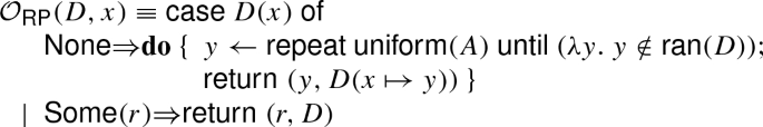
is formalised using a loop, where \({\textsf {repeat}}\ p\ {\textsf {until}}\ P\) satisfies
$$\begin{aligned} {\textsf {repeat}}\ p\ {\textsf {until}}\ P \equiv \mathbf{do }\ \{\ x \leftarrow p;\ {\textsf {if}}\ P(x)\ {\textsf {then}}\ {\textsf {return}}_{}\ x\ {\textsf {else}}\ {\textsf {repeat}}\ p\ {\textsf {until}}\ P\ \} \end{aligned}$$and \({\textsf {ran}}(D)\) denotes the range of the map \(D\). CryptHOL and EasyCrypt use \(y \leftarrow {\textsf {uniform}}(A - {\textsf {ran}}(D))\) instead of the loop. This requires an additional game hop, which accounts for 44 and 93 lines, respectively. These lines are included in the line counts in Table 1.
As observed already by Bellare and Rogaway [12], the intermediate games in a sequence of game hops need not meet any computability or efficiency constraints. It is only when we apply a hardness assumption that we must show that the reduction runs in polynomial time. Thus, by treating run-time constraints independently of the advantages, we avoid cluttering the proofs with unnecessary details about run time. This demonstrates that it is important that the semantic domains of games, adversaries, and reductions are not artificially restricted, e.g. by termination or efficiency constraints, as these constraints would have to be proven whenever a game is written down formally.

References
G. Asharov, A. Beimel, N. Makriyannis, E. Omri, Complete characterization of fairness in secure two-party computation of boolean functions, in Dodis, Y., Nielsen, J.B. (eds.) TCC 2015. LNCS, vol. 9014, (Springer, 2015), pp. 199–228
P. Audebaud, C. Paulin-Mohring, Proofs of randomized algorithms in Coq. Sci. Comput. Program. 74(8), 568–589 (2009)
F. Baader, T. Nipkow, Term Rewriting and All That. Cambridge University Press (1998)
M. Backes, M. Berg, D. Unruh, A formal language for cryptographic pseudocode, in LPAR 2008. LNCS, vol. 5330, (Springer, 2008), pp. 353–376
G. Barthe, C. Fournet, B. Grégoire, P.Y. Strub, N. Swamy, S. Zanella Béguelin, Probabilistic relational verification for cryptographic implementations. in POPL 2014. (ACM, 2014) pp. 193–205
G. Barthe, B. Grégoire, S. Heraud, S. Zanella Béguelin, Computer-aided security proofs for the working cryptographer. in CRYPTO 2011. LNCS, vol. 6841, (Springer 2011), pp. 71–90
G. Barthe, B. Grégoire, J. Hsu, P.Y. Strub, Coupling proofs are probabilistic product programs. in POPL 2017. (ACM, 2017), pp. 161–174
G. Barthe, B. Grégoire, S. Zanella Béguelin, Formal certification of code-based cryptographic proofs. in POPL 2009. (ACM, 2009), pp. 90–101
D. Basin, M. Kaufmann, The Boyer-Moore prover and Nuprl: An experimental comparison. in Huet, G., Plotkin, G. (eds.) Logical Frameworks. (Cambridge University Press, 1991), pp. 89–119
M. Bellare, A. Boldyreva, S. Micali, Public-key encryption in a multi-user setting: Security proofs and improvements. in Preneel, B. (ed.) EUROCRYPT 2000. LNCS, vol. 1807, (Springer, 2000), pp. 259–274
M. Bellare, P. Rogaway, Optimal asymmetric encryption. in Workshop on the Theory and Application of Cryptographic Techniques. (Springer, 1994), pp. 92–111
M. Bellare, P. Rogaway, Code-based game-playing proofs and the security of triple encryption. Cryptology ePrint Archive, Report 2004/331 (2004), http://eprint.iacr.org/2004/331
M. Bellare, P. Rogaway, The security of triple encryption and a framework for code-based game-playing proofs. in EUROCRYPT 2006. LNCS, vol. 4004, (Springer, 2006), pp. 409–426
J. Bengtson, K. Bhargavan, C. Fournet, A.D. Gordon, S. Maffeis, Refinement types for secure implementations. ACM Trans. Program. Lang. Syst. 33(2), 8:1–8:45 (2011)
M. Berg, Formal verification of cryptographic security proofs. Ph.D. thesis, Universität des Saarlandes (2013)
S. Berghofer, M. Wenzel, Logic-free reasoning in Isabelle/Isar. in Autexier, S., Campbell, J., Rubio, J., Sorge, V., Suzuki, M., Wiedijk, F. (eds.) CICM 2008. LNCS, vol. 5144, (Springer, 2008), pp. 355–369
K. Bhargavan, C. Fournet, M. Kohlweiss, A. Pironti, P.Y. Strub, Implementing TLS with verified cryptographic security. in S&P 2013. (IEEE, 2013), pp. 445–459
B. Blanchet, A computationally sound mechanized prover for security protocols. IEEE Trans. Dependable Secure Comput. 5(4), 193–207 (2008)
J.C. Blanchette, A. Bouzy, A. Lochbihler, A. Popescu, D. Traytel, Friends with benefits: Implementing corecursion in foundational proof assistants. in Yang, H. (ed.) ESOP 2017. LNCS, (Springer 2017), pp. 111–140
J.C. Blanchette, J. Hölzl, A. Lochbihler, L. Panny, Popescu, A., D. Traytel, Truly modular (co)datatypes for Isabelle/HOL. in ITP 2014. LNCS, vol. 8558, (Springer, 2014), pp. 93–110
D. Butler, D. Aspinall, A. Gascon, How to simulate it in Isabelle: Towards formal proof for secure multi-party computation (2017), accepted at ITP 2017
D. Butler, D. Aspinall, A. Gascón, On the formalisation of \(\varSigma \)-protocols and commitment schemes. in Nielson, F., Sands, D. (eds.) POST 2019. LNCS, vol. 11426, (Springer, 2019), pp. 175–196
R. Canetti, Universally composable security: A new paradigm for cryptographic protocols. in Proceedings of 42nd IEEE Symposium on Foundations of Computer Science, 2001. (IEEE, 2001), pp. 136–145
A. Church, A formulation of the simple theory of types. J. Symb. Log. 5(2), 56–68 (1940)
R. Cohen, S. Coretti, J. Garay, V. Zikas, Probabilistic termination and composability of cryptographic protocols. in Robshaw, M., Katz, J. (eds.) CRYPTO 2016. LNCS, vol. 9816, (Springer ,2016), pp. 240–269
Easycrypt: Reference manual. https://www.easycrypt.info/documentation/refman.pdf (2018), version 1.x, 19 February 2018
T. Elgamal, A public key cryptosystem and a signature scheme based on discrete logarithms. IEEE Transactions on Information Theory 31(4), 469–472 (1985)
S. Goldwasser, S. Micali, Probabilistic encryption. Journal of Computer and System Sciences 28(2), 270–299 (1984)
S.D. Gordon, C. Hazay, J. Katz, Y. Lindell, Complete fairness in secure two-party computation. J. ACM 58(6), 24:1–24:37 (2011)
O. Grumberg, N. Francez, S. Katz, Fair termination of communicating processes. in PODC 1984. (ACM, 1984), pp. 254–265
S. Halevi, A plausible approach to computer-aided cryptographic proofs. Cryptology ePrint Archive, Report 2005/181 (2005)
M. Hofmann, A. Karbyshev, H. Seidl, What is a pure functional? in Abramsky, S., Gavoille, C., Kirchner, C., Meyer auf der Heide, F., Spirakis, P.G. (eds.) ICALP 2010. LNCS, vol. 6199, (Springer 2010), pp. 199–210
J. Hölzl, A. Lochbihler, D. Traytel, A formalized hierarchy of probabilistic system types. in ITP 2015. LNCS, vol. 9236, (Springer, 2015), pp. 203–220
B. Huffman, O. Kunčar, Lifting and Transfer: A modular design for quotients in Isabelle/HOL. in CPP 2013. LNCS, vol. 8307, (Springer, 2013), pp. 131–146
J. Hurd, A formal approach to probabilistic termination. in TPHOLs 2002. LNCS, vol. 2410, (Springer, 2002), pp. 230–245
J. Kilian, P. Rogaway, How to protect DES against exhaustive key search (an analysis of DESX). Journal of Cryptology14(1), 17–35 (2001)
D.E. Knuth, A.C. Yao, The complexity of nonuniform random number generation. in Traub, J.F. (ed.) Algorithms and Complexity—New Directions and Recent Results. (Academic Press, Inc., 1976), pp. 357–428
N. Koblitz, A.J. Menezes, Another look at “provable security”. Journal of Cryptology 20(1), 3–37 (2007)
A. Krauss, Automating Recursive Definitions and Termination Proofs in Higher-Order Logic. Ph.D. thesis, Technische Universität München (2009)
A. Krauss, Recursive definitions of monadic functions. in PAR 2010. EPTCS, vol. 43, pp. 1–13 (2010)
O. Kunčar, A. Popescu, A consistent foundation for Isabelle/HOL. in Urban, C., Zhang, X. (eds.) ITP 2015. LNCS, vol. 9236, (Springer, 2015), pp. 234–252
O. Kunčar, A. Popescu, Comprehending Isabelle/HOL’s consistency. in Yang, H. (ed.) ESOP 2017. LNCS, vol. 10201, (Springer, 2017), pp. 724–749
O. Kunčar, A. Popescu, Safety and conservativity of definitions in HOL and Isabelle/HOL. in POPL 2018. Proc. ACM Program. Lang., vol. 2, (ACM, 2017), pp. 24:1–24:26
P. Lammich, Automatic data refinement. in ITP 2013. LNCS, vol. 7998, (Springer, 2013), pp. 84–99
K.G. Larsen, A. Skou, Bisimulation through probabilistic testing. Inf. Comp. 94(1), 1–28 (1991)
T. Lindvall, Lectures on the Coupling Method. Dover Publications, Inc. (2002)
A. Lochbihler, A formal proof of the max-flow min-cut theorem for countable networks. Archive of Formal Proofs (2016), http://isa-afp.org/entries/MFMC_Countable.shtml, Formal proof development
A. Lochbihler, Probabilistic functions and cryptographic oracles in higher order logic. in Thiemann, P. (ed.) Programming Languages and Systems (ESOP 2016). LNCS, vol. 9632, (Springer, 2016), pp. 503–531
A. Lochbihler, CryptHOL. Archive of Formal Proofs (2017), http://isa-afp.org/entries/CryptHOL.shtml, Formal proof development
A. Lochbihler, Probabilistic while loop. Archive of Formal Proofs (2017), http://isa-afp.org/entries/Probabilistic_While.html, Formal proof development
A. Lochbihler, S.R. Sefidgar, A tutorial introduction to CryptHOL. Cryptology ePrint Archive, Report 2018/941 (2018), https://eprint.iacr.org/2018/941
A. Lochbihler, S.R. Sefidgar, D.A. Basin, U. Maurer, Formalizing constructive cryptography using CryptHOL. in CSF 2019. (IEEE Computer Society, 2019), pp. 152–166
A. Lochbihler, S.R. Sefidgar, B. Bhatt, Game-based cryptography in HOL. Archive of Formal Proofs (2017), http://isa-afp.org/entries/Game_Based_Crypto.shtml, Formal proof development
A. Lochbihler, M. Züst, Programming TLS in Isabelle/HOL. Isabelle Workshop 2014 (2014)
J. Lumbroso, Optimal discrete uniform generation from coin flips, and applications. CoRR arXiv:1304.1916 (2013)
U. Maurer, Constructive cryptography – a new paradigm for security definitions and proofs. in Moedersheim, S., Palamidessi, C. (eds.) Theory of Security and Applications (TOSCA 2011). LNCS, vol. 6993, (Springer, 2011), pp. 33–56
D. Micciancio, S. Tessaro, An equational approach to secure multi-party computation. in ITCS 2013. (ACM, 2013), pp. 355–372
R. Milner, Processes: A mathematical model of computing agents. in Rose, H.E., Shepherdson, J. (eds.) Logic Colloquium 1973, Studies in Logic and the Foundations of Mathematics, vol. 80, (Elsevier, 1975), pp. 157–173
R. Milner, A theory of type polymorphism in programming. Journal of Computer and System Sciences 17(3), 348–375 (1978)
J.C. Mitchell, Representation independence and data abstraction. in POPL 1986. (ACM, 1986), pp. 263–276
T. Nipkow, G. Klein, Concrete Semantics. Springer (2014)
T. Nipkow, L.C. Paulson, M. Wenzel, Isabelle/HOL — A Proof Assistant for Higher-Order Logic, LNCS, vol. 2283. Springer (2002)
R. Pass, E. Shi, F. Tramer, Formal abstractions for attested execution secure processors. Cryptology ePrint Archive, Report 2016/1027 (2016), http://eprint.iacr.org/2016/1027
A. Petcher, G. Morrisett, The foundational cryptography framework. in POST 2015. LNCS, vol. 9036, (Springer, 2015), pp. 53–72
A. Petcher, G. Morrisett, A mechanized proof of security for searchable symmetric encryption. in CSF 2015. (IEEE 2015), pp. 481–494
M. Piróg, J. Gibbons, The coinductive resumption monad. in Jacobs, B., Silva, A., Staton, S. (eds.) MFPS 2014. ENTCS, vol. 308, (2014), pp. 273–288
A.M. Pitts, The HOL logic. in Gordon, M.J.C., Melham, T.F. (eds.) Introduction to HOL: a theorem proving environment for higher order logic, (Cambridge University Press, 1993), pp. 191–232
N. Ramsey, A. Pfeffer, Stochastic lambda calculus and monads of probability distributions. in POPL 2002. (ACM, 2002), pp. 154–165
J.C. Reynolds, Types, abstraction and parametric polymorphism. in IFIP 1983. Information Processing, vol. 83, (North-Holland/IFIP, 1983), pp. 513–523
J. Sack, L. Zhang, A general framework for probabilistic characterizing formulae. in VMCAI 2012. LNCS, vol. 7148, (Springer, 2012), pp. 396–411
N. Schirmer, M. Wenzel, State spaces – the locale way. in Huuck, R., Klein, G., Schlich, B. (eds.) SSV 2009. Electronic Notes in Theoretical Computer Science, vol. 254, (2009), pp. 161–179
R. Segala, Modeling and Verification of Randomized Distributed Real-Time Systems. Ph.D. thesis, Department of Electrical Engineering and Computer Science, Massachusetts Institute of Technology (1995)
V. Shoup, OAEP reconsidered. in Annual International Cryptology Conference. (Springer, 2001), pp. 239–259
V. Shoup, Sequences of games: A tool for taming complexity in security proofs. Cryptology ePrint Archive, Report 2004/332 (2004), http://eprint.iacr.org/2004/332
N.P. Smart, Cryptography Made Simple. Information Security and Cryptography, Springer (2016)
A. Sokolova, Coalgebraic Analysis of Probabilistic Systems. Ph.D. thesis, Technische Universiteit Eindhoven (2005)
J. Stern, D. Pointcheval, J. Malone-Lee, N.P. Smart, Flaws in applying proof methodologies to signature schemes. in Annual International Cryptology Conference. (Springer, 2002), pp. 93–110
P.Y. Strub, Some questions. Easycrypt Mailing list, post 383. https://lists.gforge.inria.fr/pipermail/easycrypt-club/2016-March/000383.html (2016)
N. Swamy, J. Chen, C. Fournet, P.Y. Strub, K. Bhargavan, J. Yang, Secure distributed programming with value-dependent types. J. Funct. Program. 23(4), 402–451 (2013)
P. Wadler, Theorems for free! in FPCA 1989. (ACM, 1989), pp. 347–359
P. Wadler, The essence of functional programming. in POPL 1992. (ACM, 1992), pp. 1–14
F. Wiedijk, A synthesis of the procedural and declarative styles of interactive theorem proving. Logical Methods in Computer Science 8(1:30), (2012)
L. Xi, K. Yang, Z. Zhang, D. Feng, DAA-related APIs in TPM 2.0 revisited. in (International Conference on Trust and Trustworthy Computing). (Springer, 2014), pp. 1–18
A.C. Yao, Theory and application of trapdoor functions. in FOCS 1982. (IEEE Computer Society, 1982), pp. 80–91
S. Zanella Béguelin, Formal Certification of Game-Based Cryptographic Proofs. Ph.D. thesis, École Nationale Supérieure des Mines de Paris (2010)
Acknowledgements
Andreas Lochbihler and S. Reza Sefidgar were supported by the Swiss National Science Foundation Grant 153217 “Formalising Computational Soundness for Protocol Implementations”.
Author information
Authors and Affiliations
Corresponding author
Additional information
Communicated by Ran Canetti.
Publisher's Note
Springer Nature remains neutral with regard to jurisdictional claims in published maps and institutional affiliations.
A preliminary version of this paper appeared at ESOP 2016 [48].
Appendices
Appendix A Further Background
This appendix provides further background to make the paper more accessible to cryptographers missing background in languages and logic. It is intended to enable them to convince themselves that cryptographic formalisations using CryptHOL have the indented meaning.
1.1 A.1 Justifying Recursive Function Definitions
Recursive function definitions must be justified to avoid inconsistencies. For example, the recursive specification  for a function \({\textsf {bad}} \mathrel {:}\mathbbm {1}\mathbin {\Rightarrow }\mathbb {N}\) must not be admitted. If it were, we could derive
  , a contradiction. So, the justification must prove that the recursion equation has a solution.
The recursive definitions in this paper are justified using three principles: well-founded recursion, least fixpoints, and primitive corecursion. Each definition principle yields a corresponding proof principle.
For well-founded recursion, the specification must be accompanied by a proof that the recursion terminates. Then, there is always a solution. Proofs about functions defined by well-founded recursion proceed by well-founded induction. In Isabelle/HOL, the \(\mathbf{function }\) package [39] is based on well-founded recursion.
For least fixpoints, a recursive specification \(f(x) \equiv \ldots f(\ldots ) \ldots x \ldots \) of a function \(f \mathrel {:}\tau _1 \mathbin {\Rightarrow }\tau _2\) is transformed into the associated functional \(F(f,x) \equiv \ldots f(\ldots ) \ldots x \ldots \), which is not recursive. If \(f\)’s codomain \(\tau _2\) is a chain-complete partial order (i.e. there is a partial order \(\sqsubseteq \) on \(\tau _2\) in which every totally ordered subset has a least upper bound) and \(F \mathrel {:}(\tau _1 \mathbin {\Rightarrow }\tau _2) \mathbin {\Rightarrow }(\tau _1 \mathbin {\Rightarrow }\tau _2)\) is monotone, then the transfinite iteration of \(F\) starting at the least element leads to the least fixpoint of \(F\), which is taken as the definition of \(f\) [40]. Proofs about least fixpoints use fixpoint induction, i.e. the property \(P\) must hold for the least element and be preserved by the functional \(F\). Fixpoint induction also demands that \(P\) be admissible, i.e. whenever \(P\) holds for all elements of a non-empty, totally ordered subset \(A\) of \(\tau _1 \mathbin {\Rightarrow }\tau _2\), then \(P\) must also hold for the least upper bound of \(A\).
In Isabelle/HOL, the \(\mathbf{partial }\text{- }\mathbf{function }\) command [40] is built on the least fixpoint principle. For example, suppose that \({\textsf {bad}}\) had the type \(\mathbbm {1}\mathbin {\Rightarrow }\mathbb {N}^\infty \) where \(\mathbb {N}^\infty \) denotes the natural numbers extended with infinitely. The least fixpoint principle could then justify \({\textsf {bad}}\)’s definition because \(\mathbb {N}^\infty \) with the usual order is a chain-complete partial order. We would get the solution  for the recursive specification. The recursive definitions in Fig. 3 are all justified by the least fixpoint principle.
Primitive corecursion is explained in Appendix A.2.
1.2 A.2 Corecursion and Coinduction
CryptHOL heavily uses coinductive definitions and proofs to handle finite and infinite objects uniformly. To make the formalisation and proofs more accessible, we briefly review the coinductive concepts that we use and compare them to their inductive counterparts using a simple example. In a nutshell, coinduction is the dual to induction.
Coinductive Datatypes. To compare inductive and coinductive definitions, consider the construction rules for binary trees with integers at the leaves:
- (a)
If \(n \mathrel {:}\mathbb {Z}\), then \({\textsf {Leaf}}(n)\) is a tree.
- (b)
If \(l\) and \(r\) are trees, then \({\textsf {Node}}(l, r)\) is a tree.
If we want to define the set \(\mathbb {T}\) of trees inductively, we say that \(\mathbb {T}\) is the smallest set that is closed under the construction rules (a) and (b). This means that every tree in \(\mathbb {T}\) is built in finitely many steps according to the above rules. Thus, \(\mathbb {T}\) contains all finite binary trees. This yields an (inductive) datatype:

Conversely, in a coinductive definition, we say that \(\overline{\mathbb {T}}\) is the largest set that is consistent with the rules (a) and (b). This means that \(\overline{\mathbb {T}}\) contains everything where we cannot rule out in finitely many steps that it was not built according to the above rules. Thus, every tree can be decomposed into either a leaf or a node with two child trees. Additionally, we identify all elements in \(\overline{\mathbb {T}}\) that cannot be distinguished by finitely many decomposition steps, i.e. bisimilar trees are considered identical. Then, \(\overline{\mathbb {T}}\) is the set of all finite and infinite binary trees. This gives a coinductive datatype (or codatatype):

Codatatypes provide a natural way to model computations. One can only observe finite parts of a computation’s behaviour, just like one can only decompose codatatypes to a finite depth. In contrast, datatypes model finite objects that can be completely analysed.
Corecursion Recursion is the primary definition principle for functions that take a datatype value as an argument, and corecursion is for functions that return a codatatype value. For example, the function \({\textsf {d}}\) below on the left computes the depth of a finite binary tree as a natural number, which is modelled as a datatype in Peano style. The function \({\textsf {max}}\) (not shown) returns the maximum of its two arguments. This recursive definition is acceptable because the recursion terminates: the subtrees \(l\) and \(r\) given to the recursive calls are strictly smaller than \({\textsf {Node}}(l, r)\) since all trees in \(\mathbb {T}\) are finite. In fact, it is even primitively recursive, because the recursive calls are on the direct arguments \(l\) and \(r\) of the constructor \({\textsf {Node}}\). In this view, \({\textsf {d}}\) destructs its argument.

On the right, \(\overline{{\textsf {d}}}\) computes the depths of trees in \(\overline{\mathbb {T}}\). As these trees may be infinite, \(\overline{{\textsf {d}}}\)’s return type is the natural numbers extended with infinity, which we model as the Peano codatatype (the infinite term \({\textsf {Suc}}({\textsf {Suc}}({\textsf {Suc}}(\ldots )))\) represents infinity). This recursive definition cannot be justified by a termination argument because the recursion does not terminate for infinite trees. Instead, corecursion on \(\mathbb {N}^\infty \) is the right definition principle. To this end, one must check that \(\overline{{\textsf {d}}}\) is productive, i.e. whenever we want to inspect \(\overline{{\textsf {d}}}\)’s output to some finite depth, \(\overline{{\textsf {d}}}\) decomposes its argument \(t \mathrel {:}\overline{\mathbb {T}}\) only to some finite depth. Here, to produce one \({\textsf {Suc}}\) constructor, \(\overline{{\textsf {d}}}\) peels off one \({\textsf {Node}}\) constructor. This definition is not primitively corecursive, because the context of the corecursive calls \(\overline{{\textsf {d}}}(l)\) and \(\overline{{\textsf {d}}}(r)\) does not consist of only one \({\textsf {Suc}}\) constructor, but also includes the \({\textsf {max}}\) function.
Coinduction. Induction requires an inductive assumption like “\(t\) is a finite tree”: If we can prove that a property \(P\) holds for all \({\textsf {Leaf}}(n)\) and is preserved by \(Node\)s, i.e. \(P\) is closed under the tree construction rules (a) and (b), then \(P\) holds for all finite trees. This proof principle is valid because \(\mathbb {T}\) is the smallest set closed under the construction rules.
In contrast, coinduction establishes a coinductive conclusion like “two trees are equal”. If we can prove that a relation \(R\) is consistent with the tree construction rules (a) and (b), then \(R\)-related trees are equal. This proof principle is valid because equality is the largest relation consistent with the construction rules (as bisimilar trees are identified).
For example, let \({\textsf {mirror}}\) be a function which swaps all left and right subtrees of all nodes in a tree. We prove \(\forall t \mathrel {:}\mathbb {T}.\ {\textsf {d}}({\textsf {mirror}}(t)) = {\textsf {d}}(t)\) by induction on the inductive assumption \(t \mathrel {:}\mathbb {T}\). Conversely, \(\forall t \mathrel {:}\overline{\mathbb {T}}.\ \overline{{\textsf {d}}}({\textsf {mirror}}(t)) = {\textsf {d}}(t)\) is proven by coinduction on the coinductive equality relation on \(\mathbb {N}^\infty \).
1.3 A.3 Relational Parametricity and Representation Independence
A function like \(\pi _1\mathrel {:}\alpha \mathbin {\times }\beta \mathbin {\Rightarrow }\alpha \) is polymorphic in a type variable \(\alpha \) if its behaviour does not depend on the actual type of the argument, i.e. the function behaves uniformly for all type instances. Reynolds [69] and Wadler [80] formalised this notion of independence using relational parametricity. They interpret the type of a function as a relation between values instead of a set of values. Type constructors without type arguments like \(\mathbb {B}\), \(\mathbb {N}\), and \(\mathbb {R}\) become the identity relation on the set of values, which we denote by \({\widetilde{\mathbb {B}}}\), \({\widetilde{\mathbb {N}}}\), and \({\widetilde{\mathbb {R}}}\), respectively. Type constructors with type arguments like \(\mathbin {\times }\) and \(\mathbin {\Rightarrow }\) become relation transformers, i.e. functions from relations to relations, which we write with a \(\widetilde{~}\) over the type constructor. For example, \((\mathbin {{\widetilde{\mathord {\mathbin {\times }}}}}) \mathrel {:}\mathbb {P}(\alpha \mathbin {\times }\alpha ') \mathbin {\Rightarrow }\mathbb {P}(\beta \mathbin {\times }\beta ') \mathbin {\Rightarrow }\mathbb {P}((\alpha \mathbin {\times }\beta ) \mathbin {\times }(\alpha ' \mathbin {\times }\beta '))\) lifts two relations component-wise to pairs. Formally, \((x, y) \mathrel {(A \mathbin {{\widetilde{\mathord {\mathbin {\times }}}}}B)} (x', y')\) iff \(x \mathrel {A} x'\) and \(y \mathrel {B} y'\). Similarly,  for the function space relates two functions \(f\) and \(g\) iff they transform relatedness in \(A\) into relatedness in \(B\). Formally,
  iff \(f(x) \mathrel {B} g(y)\) whenever \(x \mathrel {A} y\). Now, a function is relationally parametric in a type variable \(\alpha \) iff it is related to itself in the relation that corresponds to its type where \(\alpha \) is interpreted by an arbitrary relation \(A\). For example, \(\pi _1\) being parametric in \(\alpha \) and \(\beta \) is expressed by

Note the similarity between \(\pi _1\)’s type and the relation. We list the relators for further type constructors:
Sums\({\textsf {Left}}(x) \mathrel {(A \mathbin {{\widetilde{\mathord {\mathord {+}}}}}B)} {\textsf {Left}}(y)\) iff \(x \mathrel {A} y\), and \({\textsf {Right}}(x) \mathrel {(A \mathbin {{\widetilde{\mathord {\mathord {+}}}}}B)} {\textsf {Right}}(y)\) iff \(x \mathrel {B} y\), but \(\mathbin {{\widetilde{\mathord {\mathord {+}}}}}\) does not relate \({\textsf {Left}}(\_)\) and \({\textsf {Right}}(\_)\).
Sets\(X \mathrel {{\widetilde{\mathbb {P}}}(R)} Y\) iff \(R[X] \subseteq Y\) and \(R^{-1}[Y] \subseteq X\).
Maybe\({\widetilde{\mathbb {M}}}(A)\) relates \({\textsf {None}}\) to \({\textsf {None}}\), and \(\textsf {Some}(x)\) to \(\textsf {Some}(y)\) whenever \(x \mathrel {A} y\), and nothing else.
Wadler [80] proved that all functions definable in the polymorphic lambda calculus are parametric. He also demonstrated that adding polymorphic equality destroys this property. Higher-order logic has polymorphic equality \((\mathord {=})\) and description operators, so not all HOL functions are parametric. Thus, parametricity is not a free theorem in our setting; we must prove it for every constant. Fortunately, function application and function composition preserve parametricity. Hence, functions defined in terms of parametric functions are parametric too.
Wadler also showed that if all types are \(\omega \)-ccpos, all functions are continuous and all relations are admissible and strict, then the fixpoint operator (defined by countable iteration) is parametric [80]. We do not consider the fixpoint operator as part of the language itself, but as a definition principle for recursive user-specified functions. That is, we assume that \({\textsf {fix}}\) is always applied to a monotone function. Thus, preservation of parametricity (Theorem 1) suffices and we do not need Wadler’s restrictions of the semantic domains. So, monotonicity (instead of continuity as discussed in Sect. 4.2) is expressed as a precondition on the given functions.
Wadler’s free theorems express that parametric functions commute with the lift operation \(\widehat{~}\). For example, we get \(\pi _1( xy \rhd (f \mathbin {\widehat{\mathbin {\times }}}g)) = f(\pi _1( xy ))\) from (18) by instantiating \(A\) and \(B\) with the graphs of the functions \(f\) and \(g\), respectively, and by unfolding the definitions of \(\mathbin {\widehat{\mathbin {\times }}}\) and the relators. Wadler calls this a free theorem because we do not need any property of \(\pi _1\) other than (18); in particular, we do not need to unfold \(\pi _1\)’s definition. In this tiny example, it might have been easier to unfold the definition, but for complicated function definitions, proofs by parametricity are more systematic and therefore automatic.
Representation independence [60] expresses that changing the implementation of a module in a program does not affect the overall result. Mitchell uses parametricity to formalise this notion as follows. If we can find a bisimulation relation for all functions in the interface of the module being changed, and the remainder of the program is parametric in the type defined by the module, then the change does not affect the program. That is, representation independence lifts bisimilarity over contexts using parametricity. For example, consider a deterministic transducer given by its transition function \(\delta \mathrel {:}\sigma \mathbin {\Rightarrow }\alpha \mathbin {\Rightarrow }\beta \mathbin {\times }\sigma \), which, given a state \(s \mathrel {:}\sigma \) and a input letter \(x \mathrel {:}\alpha \), computes an output letter from the output alphabet \(\beta \) and the successor state. This is the interface of the module. The recursive function \({\textsf {run}}_{\delta }\) given below computes a run of the transducer with transition function \(\delta \) from state \(s\) on the input word \(w \mathrel {:}\mathbb {L}(\alpha )\).
This is the context of the transducer module. Note that \({\textsf {run}}_{}\) is parametric in the state space, i.e.

for all \(S\). Now, representation independence says that we can replace the transducer \(\delta _1\) by a bisimilar one \(\delta _2\) (and the initial state \(s_1\) by \(s_2\)) without changing the overall result. Here, bisimilarity means that we find a bisimulation relation \(S\) between the states of the two transducers, i.e. (i) \(S\) relates the initial states \(s_1\) and \(s_2\), and (ii) whenever \(S\) relates two states \(s_1\) and \(s_2\) and for all inputs \(x\), the transition functions \(\delta (s_1, x)\) and \(\delta (s_2, x)\) return the same output and successor states which \(S\) relates. As parametricity is compositional, this result scales to arbitrarily large contexts, not just a small function like \({\textsf {run}}_{}\).
In Isabelle, the transfer package [34] implements representation independence as a proof engine. That is, having proven bisimilarity of two particular transition functions, a single invocation of this engine lifts the bisimilarity property over arbitrarily large contexts.
B Proofs
1.1 B.1 Subprobabilities are a CCPO
Proof of Proposition 1
We have to show that \(\mathrel \sqsubseteq \) is a partial order and that \(\bigsqcup {Y}\) is well defined and the least upper bound for every chain \(Y\), i.e. every set of spmfs all of whose elements are comparable in \(\mathrel \sqsubseteq \). The difficult part is to show that \(\bigsqcup {Y}\) is well defined. In particular, we must show that the support of \(\bigsqcup Y\) is countable even if \(Y\) is uncountable. Then, it is not hard to see that \(\bigsqcup {Y}\) sums up to at most 1.
Clearly, we have \({\textsf {support}}\left( \bigsqcup Y\right) = \cup _{p \in Y} {\textsf {support}}(p)\). Yet, the union of an uncountable sequence of increasing countable sets need not be countable in general. In the following, we show that even for uncountable chains \(Y\) of spmfs, the union of the supports remains countable. To this end, we identify a countable sub-sequence of \(Y\) whose lub has the same support. The key idea is that for \(\mathrel \sqsubseteq \)-comparable spmfs \(p\) and \(q\), the order can be decided by looking only at the assigned probability masses, namely \(p \mathrel \sqsubseteq q\) iff \(\Vert p\Vert \le \Vert q\Vert \). So suppose without loss of generality that \(Y\) does not contain a maximal element (otherwise, the lub is the maximal element and we are done). The set of assigned probability masses \(A = \{\,\Vert p\Vert \mid p \in Y\,\}\) has a supremum \(r \le 1\), as \(1\) bounds the set from above. The closure of \(A\) contains the supremum \(r\), so \(A\) must contain a countable increasing sequence which converges to \(r\). This sequence gives rise to a countable sub-sequence \(Z\) of \(Y\), for which we show \((\cup _{p \in Y} {\textsf {support}}(p)) \subseteq (\cup _{q \in Z} {\textsf {support}}(q))\). For any \(p \in Y\), there is a \(q \in Z\) such that \(\Vert p\Vert \le \Vert q\Vert \), as the assigned probability masses in \(Z\) converge to \(r\) from below and \(p\) is not maximal. Hence, \(p \mathrel \sqsubseteq q\) as \(p\) and \(q\) are related in \(\mathrel \sqsubseteq \), and therefore \({\textsf {support}}(p) \subseteq {\textsf {support}}(q)\) as \({\textsf {support}}\) is monotone. \(\square \)
The attentive reader might wonder why we need transfinite iteration for the fixpoint despite having shown that uncountable chains can be reduced to countable ones for the purpose of lubs. Countable fixpoint iteration, which defines the least fixpoint as \(\bigsqcup \{\,f^i(\mathord {\bot }) \mid i \in \mathbb {N}\,\}\), does not suffice. (Here, function iteration is defined by \(f^0 = {\textsf {id}}\) and \(f^{n+1} = f \circ f^n\).) The reason is that the chain \(\{\,f^i(\mathord {\bot }) \mid i \in \mathbb {N}\,\}\) might stop before the least fixpoint is reached. Consider, e.g. the monotone spmf transformer \(f \mathrel {:}\mathbb {D}(\mathbbm {1}) \mathbin {\Rightarrow }\mathbb {D}(\mathbbm {1})\) given by
The countable iteration of \(f\) starting at \(\mathord {\bot }\) yields a sequence of spmfs which assign to  the masses \(0\), \(\frac{1}{4}\), \(\frac{3}{8}\), \(\frac{7}{16}\), \(\frac{15}{32}\), ... The least upper bound of this sequence assigns \(\frac{1}{2}\) to
  . That is, the iteration has not yet reached \(f\)’s fixed point, which assigns the mass \(1\) to
  . This is because \(f\) is not (chain) continuous, i.e. it does not preserve lubs.
1.2 B.2 Fixpoints Preserve Parametricity
A relation \(R \mathrel {:}\mathbb {P}(A \mathbin {\times }B)\) is admissible w.r.t. two ccpos iff for any chain \(Y \subseteq R\) of pairs in the product ccpo (the ordering is component-wise), \(R\) relates the component-wise lubs of \(Y\).
Proof of Theorem 1
We prove Theorem 1 by parallel induction on the two fixpoints. Both inductive cases are trivial. The base case requires \({\widetilde{\mathbb {D}}}(R)\) to be strict, i.e. it relates the least elements, which holds trivially. The step case is precisely the relatedness condition of \(f\) and \(g\), which the theorem assumes. Parallel fixpoint induction is a valid proof principle because \({\widetilde{\mathbb {D}}}(R)\) is admissible by Proposition 4. \(\square \)
Proposition 4
\({\widetilde{\mathbb {D}}}(\_)\) is admissible.
Proof
We exploit the characterisation of \({\widetilde{\mathbb {D}}}\) in terms of  . We must show \((\bigsqcup {(Y \rhd ^{\widehat{\mathbb {P}}} \pi _1)}) \mathrel {{\widetilde{\mathbb {D}}}(R)} (\bigsqcup {(Y \rhd ^{\widehat{\mathbb {P}}} \pi _2)})\) for all chains \(Y\) of pairs in \({\widetilde{\mathbb {D}}}(R)\). By the characterisation of \({\widetilde{\mathbb {D}}}\) (Lemma 1), this holds as follows: The first and last steps exploit that the lub commutes with
  , and the inequality follows from monotonicity of \({\textsf {SUP}}\) and the characterisation of \({\widetilde{\mathbb {D}}}\) for elements of the chain.

\(\square \)
Note that it is not clear how to prove admissibility via the characterisation in terms of couplings. The problem is that the couplings for the pairs in the chain need not form a chain themselves. So we cannot construct the coupling for the lubs as the lub of the couplings.
Admissibility of relators is preserved by the function space (ordered point-wise) and products (ordered component-wise).
C Guide for CryptHOL source syntax
The notation in this article is intended to make the presentation easy to follow. The CryptHOL source code and examples in the Archive of Formal Proofs [49, 53] use a somewhat different notation that follows Isabelle/HOL conventions. To help the reader to navigate the sources, this appendix relates the different notations.
Type constructors are written as a single letter in blackboard style in this article, whereas they are spelled out in words in the sources. Table 2 lists the correspondences. The notation for infix type constructors (products \(\mathbin {\times }\), sums \(\mathbin {+}\), and function space \(\mathbin {\Rightarrow }\)) remains the same. Moreover, type constructors are written in postfix in Isabelle and type variables start with a prime \({}'\), and type annotations use a double colon \(\mathbin {::}\) instead of a single colon \(\mathrel {:}\). For example, what is written \(p \mathrel {:}\mathbb {D}(\mathbb {L}(\alpha ) \mathbin {\times }\beta )\) in this article becomes \(p \mathbin {::} ({}'\!\alpha \ {\textsf {list}} \mathbin {\times }{}'\beta )\ {\textsf {spmf}}\) in the sources.
Function application is written without parentheses in Isabelle, but compound arguments must be parenthesised. Forward function application is rarely used. For example, \(f( arg _1, arg _2, g(x, y), arg _4) \rhd h\ z\) becomes \(h\ z\ (f\ arg _1\ arg _2\ (g\ x\ y)\ arg _4)\). Indices and function parameters in superscripts become ordinary function arguments, too. For instance, \(\mathcal {O}_{{\textsf {enc}}}^{k, b}(L, (m_1, m_0))\) in Sect. 6.1 is a HOL function applied to four arguments: \({\textsf {oracle\text{- }encrypt}}\ k\ b\ L\ (m_1, m_0)\), namely a key \(k\), a bit \(b\), a storage \(L\), and a pair of messages \((m_1, m_0)\). In this article, we have moved the first two into superscripts to indicate that they are actually function parameters. Relations are modelled as binary predicates, i.e. functions of type \(\alpha \mathbin {\Rightarrow }\beta \mathbin {\Rightarrow }\mathbb {B}\), rather than sets of pairs, and are usually written prefix instead of infix.
Locale instantiation in Isabelle marks the name prefix with a single colon : instead of \(\equiv \) and locale parameters are not parenthesised, like for functions. For example, \( \mathbf{sublocale }\ {\textsf {concrete}} \equiv {\textsf {ELGAMAL}}(\mathcal {G}(\eta ))\ \mathbf{for }\ \eta \) from Fig. 2 is actually written as \( \mathbf{sublocale }\ {\textsf {concrete}}:{\textsf {ELGAMAL}}\ \text {``}\mathcal {G}\ \eta \text {''}\ \mathbf{for }\ \eta \).
Lifting of functions and relations over type constructors is expressed as ordinary HOL functions with the following naming convention. A function \({\textsf {map}}\text{- }\tau \) lifts functions over the type constructor \(\tau \), and the operator \({\textsf {rel}}\text{- }\tau \) does so for relations. For example, \(\widehat{\mathbb {D}}(f)\) and \({\widetilde{\mathbb {D}}}(R)\) are written as \({\textsf {map}}\text{- }{\textsf {spmf}}\ f\) and \({\textsf {rel}}\text{- }{\textsf {spmf}}\ R\), respectively. The exception are lists with \({\textsf {map}}\) and \({\textsf {list}}\text{- }{\textsf {all2}}\), pairs with \({\textsf {map}}\text{- }{\textsf {prod}}\) and \({\textsf {rel}}\text{- }{\textsf {prod}}\), sums with \({\textsf {map}}\text{- }{\textsf {sum}}\) and \({\textsf {rel}}\text{- }{\textsf {sum}}\), and functions with \((\mathbin {\mathord {-}\mathord {-}\mathord {-}\mathord {>}})\) and \((\mathbin {\mathord {=}\mathord {=}\mathord {=}\mathord {>}})\). For example, relational parametricity of the first projection on pairs (18) is written as \( \forall A\ B.\ ({\textsf {rel}}\text{- }{\textsf {prod}}\ A\ B \mathbin {\mathord {=}\mathord {=}\mathord {=}\mathord {>}} A)\ {\textsf {fst}}\ {\textsf {fst}} \), where \({\textsf {fst}}\) is Isabelle’s notation for \(\pi _1\).
Some functions have different names and notation in the CryptHOL sources. Table 3 lists the most important differences. Changes in capitalisation and for definitions in the examples and case studies are not shown. Table 4 lists the files where the examples can be found in the sources.
Rights and permissions
About this article

Cite this article
Basin, D.A., Lochbihler, A. & Sefidgar, S.R. CryptHOL: Game-Based Proofs in Higher-Order Logic. J Cryptol 33, 494–566 (2020). https://doi.org/10.1007/s00145-019-09341-z
Received:
Revised:
Published:
Issue Date:
DOI: https://doi.org/10.1007/s00145-019-09341-z