
Abstract
We take advantage of the interpretation of stochastic capacity expansion problems as stochastic equilibrium models for assessing the risk exposure of new equipment in a competitive electricity economy. We develop our analysis on a standard multistage generation capacity expansion problem. We focus on the formulation with nonanticipativity constraints and show that their dual variables can be interpreted as the net margin accruing to plants in the different states of the world. We then propose a procedure to estimate the distribution of the Lagrange multipliers of the nonanticipativity constraints associated with first stage decisions; this gives us the distribution of the discounted cash flow of profitable plants in that stage.


Notes
Traditionally (Eisner and Olsen 1975; Rockafellar and Wets 1976; Shapiro et al. 2009), nonanticipativity constraints have been introduced for the nested formulation of the stochastic problem, i.e., letting \(x_t(\cdot )\) depend on the whole data vector \(\xi _{[T]}\). This formulation is not well suited for our purposes because it destroys the recursive pattern of the cost-to-go functions.
Based on the fact that \(\mathbb E _{\vert \xi _{[t]}} \{x_t(\xi _{[t+1]})- \mathbb E [x_t(\xi _{[t+1]})] \} =0\) and hence replacing \(\lambda _t(\xi _{[t+1]})\) with \(\lambda _t(\xi _{[t+1]})- \mathbb E [\lambda _t(\xi _{[t+1]})\vert \xi _{[t]}]\) does not change the Lagrangian (2.11) (Shapiro et al. 2009, p. 83).
The interchangeability of the operators is valid because the cost-to-go functions are convex and finite valued (Shapiro et al. 2009, Theorem 7.46)
The estimation of the Lagrange multipliers does not require a specific algorithm to compute \(\bar{x}_t(\xi _{[t]})\).
The load duration curve measures the number of hours per year the total load is at or above any given level of demand (definition taken from Steven Stoft 2002).
The complementarity notation \(0 \le x \bot y \ge 0\) stands for \(x \ge 0, y \ge 0\) and \(x \cdot y=0\).
This contrasts with the now standard missing money argument (Paul Joskow 2007) that pure market operations cannot spontaneously develop the required capacity because of an insufficient remuneration of plant in case of high demand or high plant failure. The response of the proponents of the energy only market is that one must price electricity in every state of the world at the cost that it implies, whether this is the cost of the most expensive operating unit or the cost of demand curtailment.
The risk implied by renewable policy stems from the ambitious objectives of the EU and the historical record that its plans do not always materialize as expected.
The number and the duration of the time segments are identical for all the time period \(t=1,\ldots ,T\)
The wind regimes are obtained from actual wind speed measured in 2010 in the center of Germany (\(51^\circ \) N, \(9^\circ \) E) by the National Centre for Environmental Prediction (NCEP) and applying the output function of an offshore wind turbine. Our model neglects spatial smoothing effects and exacerbates the difference between the wind efficiency regimes.
Table 2 Initial demand We used SAA and quasi-Monte Carlo sampling to solve the stochastic programs. A sample of 196 scenario is used for the transition from one stage to the next one (in total \(196^2\) states of the world in the third stage) in the computation of the first stage solution. The lower bound estimate was computed by solving 50 instances of problem.
Table 3 Wind regimes Table 4 Capacities invested in the different technologies These distribution are obtained as the distribution of the Lagrange multipliers of the nonanticipativity constraints. It is computationally convenient not to explicitly solve the extensive form of the nonanticipativity formulation but to compute the Lagrange multiplier using (2.17). We applied the procedure described in 2.2 to estimate \(\bar{\lambda }_1\), using a more extended sampling (\(77^2\)) for the second stage data vector \(\xi _2\).
Fig. 1 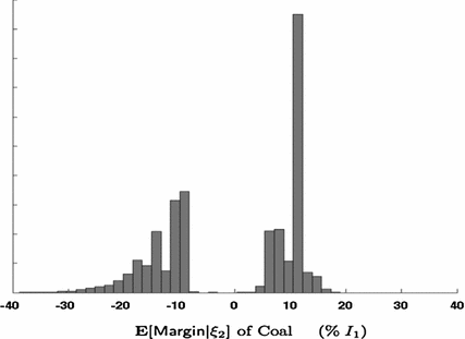
Histogram of coal margins
Fig. 2 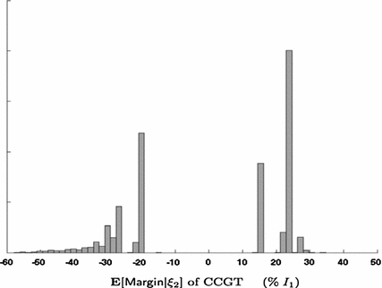
Histogram of CCGT margins
\(\mathsf CVaR ( \mathbb E [\mathrm Margin \vert \xi _2] \vert \xi 1)\) is a time-consistent risk measure


References
Ehrenmann A, Smeers Y (2011) Stochastic equilibrium models for generation capacity expansion. In: Consigli M Bertochi G, Dempster M (eds) Handbook on stochastic optimization methods in finance and energy. Springer, Berlin, pp 273–309
Eisner MJ, Olsen P (1975) Duality for stochastic programming interpreted as l.p. in \(l_p\)-space. SIAM J Appl Math 28:779–792
Joskow Paul (2007) Competitive electricity markets and investment in new generation capacity. In: Helm D (ed) The new energy paradigm. Oxford University Press, Oxford
Morlat G, Bessière F (eds) (1971) Vingt cinq ans d’Economie électrique. Dunod, Paris
Pereira MVF, Pinto LMVG (1991) Multi-stage stochastic optimization applied to energy planning. Math Program 52:359–375
Philpott AB, Guan Z (2008) On the convergence of sampling-based methods for multi-stage stochastic linear programs. Oper Res Lett 36:450–455
Rockafellar RT, Wets RJ-B (1976) Stochastic convex programming: basic duality. Pac J Math 62:173–195
Shapiro A (2003) Inference of statistical bounds for multistage stochastic programming problems. Math Methods Oper Res 58:57–68
Shapiro A (2006) On conplexity of multistage stochastic programs. Oper Res Lett 24:1–8
Shapiro A (2011a) Analysis of stochastic dual dynamic programming method. Eur J Oper Res 209(1):63–72
Shapiro A (2011b) Topics in stochastic programming. Universite Catholique de Louvain, CORE lecture series
Shapiro A, Dentcheva D, Ruszczynski A (2009) Lectures on stochastic programming: modeling and theory. SIAM, Philadelphia, PA
Stoft Steven (2002) Power system economics. Wiley-Interscience, London
Author information
Authors and Affiliations
Corresponding author
Additional information
Gauthier de Maere d’Aertrycke was partly supported by a grant from GDF-Suez. Alexander Shapiro was partly supported by the NSF award DMS-0914785 and ONR award N000140811104.
Appendix: Dual problem
Appendix: Dual problem
The optimal solutions of the Lagrangian dual problem (\(\bar{\beta }_t(\xi _{[t]}),\bar{\pi }_t(\xi _{[t]}),\bar{\mu }_t(\xi _{[t]})\) ) are obtained by solving
Rights and permissions
About this article
Cite this article
de Maere d’Aertrycke, G., Shapiro, A. & Smeers, Y. Risk exposure and Lagrange multipliers of nonanticipativity constraints in multistage stochastic problems. Math Meth Oper Res 77, 393–405 (2013). https://doi.org/10.1007/s00186-012-0423-4
Received:
Accepted:
Published:
Issue Date:
DOI: https://doi.org/10.1007/s00186-012-0423-4