
Abstract
As the human–robot interaction is catching eye day by day with the increase in need of automation in every field, personal robots are increasing in every area which may be coping needs of elderly people, treating autistic patients or child therapy, even in the area of babysitting the child. As robots are helping human being in all such cases, robots need to understand human emotion in order to treat human in a more customized manner. Predicting human emotion has been a difficult problem which is being solved over a decade’s time. In this paper, we have built a model which can predict human emotion from an image in real time. The network build is based on convolutional neural network which has reduced parameters by 90× from that of Vanilla CNN and also 50× from the latest state-of-the-art research carried out to the best of our knowledge. The network build is tested robustly on 8 different datasets, namely Fer2013, CK and CK+, Chicago Face Database, JAFFE Dataset, FEI face dataset, IMFDB, TFEID and custom dataset build in our laboratory having different angles, faces, backgrounds and age groups. The network achieves 74% accuracy which is an improved accuracy from the state-of-the-art accuracy with reduced computation complexity.
We’re sorry, something doesn't seem to be working properly.
Please try refreshing the page. If that doesn't work, please contact support so we can address the problem.
1 Introduction
Human–robot interaction is very important in this developing era of robots. Personal robots are built to help elderly people and educate children; many psychological counseling such as treating autistic patient is being conducted by personal robot. Personal robots are built such that it can work in a customized manner to gain the confidence of the person who it is dealing with. This interaction with robot requires communication with robots via speech and/or gestures. Such type of interaction can be made more fruitful once robots are able to understand human emotions. Human brain builds a facial emotion and manipulates it in a very crucial manner where emotion changes instantly as per the human mood or sentiment of the statement said or heard by the person. Human mind also predicts the emotion of the other person very efficiently depending on the mood of the person in front of her/him.
Deep learning is trying to mimic human brain to an extent closest possible. Convolutional neural network works very well on vision-based applications. When a personal robot will be able to closely understand human emotion, human will attain more confidence when interacting with robots or when relying on robots.
Human body gestures are very crucial as well as very difficult part with lots of meaning to it, out of which human facial emotion is the most crucial. It tells exactly how the person responds to any situation. So when a robot understands human emotion, it will be able to connect with human on their sentiments and hence can educate, or perform counseling in a better way.
Research tells for a human to understand other human’s emotion is still as effective as 65 ± 5% which was tested over FER 2013 dataset [1]. Research has been carried out using various methods to predict human emotion. Achieving real-time accuracy is still a challenge. Complexity of predicting human emotion can be judged simply by manually predicting the emotion from the dataset FER 2013.
In the past research, network using CNN, SVM and even probabilistic techniques has been built to predict the emotion. Problem faced in those solutions is sometimes meeting accuracy constraints, and most of the time deep learning network built has such huge parameter requirements, which made it nearly impossible to be implementable in real-time systems.
In order to be able to make instant predictions, real-time implementable system is needed in people’s daily life. Even people with development disabilities need some assistance in their daily routines. Authors in [2] have described a Canadian Survey on Disability (CSD), 2012, which states 90% of the disabled Canadian adults need assistance in daily life and 72% of them are not able to meet their need in at least one of their activities. All such daily needs and regular counseling require customizable personal robots that can interact with human by gaining their trusts and the person can rely on them. People with development disabilities are in a need for social robots which can assist the person in every phase of her/his life. An attempt is made in [2] to achieve such kind of robots. One such application is implemented for prediction of target location using the dataset of images which has finger pointing direction for robotics domain [3].
Also for normal human beings, in their daily routines the idea of smart homes can be created smarter when robots themselves can analyze human emotion and maintain the environment accordingly. Adjusting home lights, music genre and music volumes can be maintained by robots to increase human ease.
For all such application requirements, we have built a CNN model mostly inspired by inception module [4] and targeting to make it feasible for implementing in real-time system like personal robots. We have created a robust model to be used in embedded systems or robots as we have tested it in 8 different datasets, namely Fer2013, CK and CK+ , Chicago Face Database, JAFFE Dataset, FEI face dataset, IMFDB, TFEID and custom dataset build in our laboratory. We have incorporated various methods in our network to reduce computational complexity and achieve state-of-the-art accuracy. In short, we have mainly emphasized on making a robust system real time implementable on a robot.
Further, in Sect. 2, we have discussed the related work stating the state of the art carried out so far and techniques used to achieve expression detection. Section 3 discusses the methods used to build our network and make it computationally less expensive, thereby achieving state-of-the-art accuracy. In Sect. 4, we have described the analysis of our network including dataset details, experiment details, computational details and result obtained. Conclusion and future work are discussed in Sect. 5.
2 Related work
Deep learning has resolved problems in various domains [5], where earlier methods required extracting information from data manually and accordingly make decision based on a set of rules. In the earlier methods, human-prone error is very much liable to occur, and also after that, decision is made based on a human-built set of rules, which also might not be all time correct. In the case of classifying human facial emotion, researchers have built many networks using many techniques like support vector machine [6], principal component analysis [9], convolutional neural networks [7, 8].
Many sensors are also used for facial emotion recognition. Some researchers have used EEG signals [10] to predict human emotion. It recorded signals using wavelet entropy to classify human emotions. Authors are using wireless signals to predict human emotion and work accordingly. Their system works by extracting heartbeat from the wireless signals, thereby achieving accuracy equivalent to that from the ECG signals. This required infrastructure like base stations, wireless access points and reachable signals. But facial expressions play a vital role in deciding human emotion. Emotions are classified using neurophysiological data [11] where brain wave bands are used to categorize different emotions.
Lopes et al. [12] have built a convolutional network to predict emotion of the person. This proposed method requires few preprocessing of the data before predicting the emotion like spatial normalization, synthetic sample generation, image cropping, down sampling, intensity normalization. After all these steps, the resultant image is fed to CNN Network to predict the emotion which would be difficult for a robot to be feasible in real time. Authors in [13] have also implemented sentiment analysis network for a group of people using CNN and LSTM network, thereby achieving 62% accuracy approximately. In [14], authors have built a deep convolutional network to classify the emotions.
In [7], a network of convolutional layers and fully connected layers was built for emotion classification which required some preprocessing of the data before training or testing it in real time. In [8], authors have built a CNN model over raw pixel data combined with HOG (histogram of oriented gradients) features. Progressively by adding layers and varying parameters, they have come up to a stable model for classifying emotions. Dropout and regularization techniques were used to generalize the training. As fully connected layers require huge parameters, authors in [15] have replaced classification part of the CNN model with SVM to reduce parameters and the network will be more feasible for implementation in real-time applications. CNN model and representational auto encoders are also used to build a model for classifying 7 emotions in [16]. Here the authors have built a Vanilla CNN model with three layers of convolution and 2 fully connected layers to classify the emotion and have tested their system on JAFEE dataset. Such a network has millions of parameters, thereby restricting their train time, and has higher computational complexity. In [17], authors have built a deep convolutional neural network to take care of physiological data and its corresponding facial expression dataset to detect human emotion using DEAP dataset.
CNN with SVM model is built and tested over 9 different datasets to validate its robustness in [15]. In [18], authors have built a network using Alex Net to extract the features and SVM classifier to classify the emotion in the image. A survey in various emotion detection systems built is carried out in [19] to compare efficiency and complexity of the systems. They have provided a brief review about all the networks built for facial emotion recognition including traditional approaches and deep learning techniques. Various networks built include inception module and CNN network including ResNet combined with LSTM and RNN. Octavio et al. [20] have created two models based on CNN architecture to reduce hyperparameter requirement and met state-of-the-art accuracy to be feasible to run in real-time systems. Models built have reduced parameters and hence reduced computational complexity. They have worked on reducing parameters by using separable convolutions and by replacing dense layers in CNN with global average pooling.
In [21], authors have built emotion classifier by building some patterns by gradients of the neighboring pixels. Classifying the emotion in this system needs facial image to be preprocessed to a specific size, and also light effects and environment might bring changes in the pattern, thus creating ambiguity in the emotion prediction. Though this method is also achieving good results, it can be clubbed with deep learning networks to perform better. In [22], Hamdi et al. have built a deep learning network to classify features and SVM classifier to predict the taste liking through facial expressions in taste-induced expressions. Song et al. [10] have built a dynamical graph convolutional neural network to train emotion classifier on EEG dataset where they have built adjacency matrix for different EEG channels for a particular emotion and trained the CNN over it.
Authors in [23] have built a network using 3DCNN to learn spatiotemporal features, and then, convolutional LSTM is implemented to learn semantic information using longer spatiotemporal dependencies.
We have built a model based on inception module [4] and focused on reducing the network complexity, thereby achieving the state-of-the-art accuracy. Many work around was carried out before finalizing on the network architecture in order to maintain a trade-off between network complexity and accuracy. The network was trained, tested and validated on 8 different datasets to validate its robustness. The network has 90× reduced trainable parameters as compared to normal CNN model and 50× reduced parameters as compared to the best state-of-the-art network created in [20]. To the best of our knowledge, this work is not build or published elsewhere. The network was finally implemented to test in real-time environment to verify its feasibility in robotics domain.
3 Methods
We have proposed a CNN-based model and compared its computation cost and efficiency over 8 different datasets to ensure its robustness. Reason for using multiple datasets is to validate our proposed network rigorously and make a benchmark for emotion classifier over efficiency and computation cost of the system. Computational cost is reduced to an extent of up to 90% from Vanilla CNN network. And from the latest research in [15] the parameter requirement is reduced to 1.4 lakhs which is 50% reduction from the most efficient network build for emotion classification to the best of our knowledge.
3.1 Convolutional neural network
Convolution neural network is used to process image dataset and extract features in the form of edges to be able to perform classification tasks over the edge features without depending on the human-predicted features. Performing convolutions help share parameters (filter values) and are translation invariant and hence can detect features with lesser computation [24] as compared to fully connected networks and are able to detect translated features as well.
Convolutional neural network proves to be one of the best networks to process static images, given achieved accuracy, computational cost, ability to handle variable size images, not required to change network when your dataset changes, and process data in batches. CNN can manage variable kind of dataset (variable in size and quality) with requirement of least preprocessing as compared to other networks like multi-layer perceptron and recurrent neural network [25].
3.2 Inception module
Inspired by the inception module [4] shown in Fig. 1, we have implemented 1 × 1 convolutions in our model in order to reduce the dimensionality before undergoing bigger convolutions. This helps reduce the multiplications by a factor of 10 [4], hence reducing the computational complexity of the network.

Inception module to reduce dimensionality and showing use of 1 × 1 convolutions
In our network to improve upon the performance, we need not to decide which convolution to use to be able to extract the best features, use various convolutions and let the network decide what will work best. This concept is used to build our network shown in Fig. 2, inspired by inception module shown in Fig. 1.

Network architecture built to detect human emotions
4 Experiment details and result analysis
Here, we will be discussing all the datasets used to train, test and validate our network and the experiment details including parameters and various layers included in our model. We will be describing what all techniques are used to minimize the parameter requirement, thereby achieving the state-of-the-art accuracy. Finally, the result obtained is discussed.
To reduce the hyperparameter requirement, various measures are used in the network which is discussed later in this section. Mathematically, it is explained what measures are causing the network to be computationally less expensive while achieving the state-of-the-art accuracy.
4.1 Dataset used
Robust analysis is carried out to verify the network efficiency using 8 different annotated datasets. Datasets used are: Fer2013 [26], CK and CK+ [27], Chicago Face Database [28], JAFFE dataset [29], FEI face dataset [30], IMFDB [31], TFEID [32] and custom dataset build in our laboratory.
FER2013 dataset has 28,709 images for training and 3589 test images. Emotion labels and the number of images in each label are: 4593 images for angry, 5121 for fear, 547 for disgust, 8989 images for happy, 6077 for sad, 4002 images for surprise, and 6198 images are neutral emotion. Cohn-Kanade+ (CK+) dataset consists of 593 sequence of images showing 7 emotions from 123 targets.
Chicago face database consists of black and white images of various individuals. Targets in the database have 5 labels: neutral, angry, happy (with open mouth), happy (with closed mouth) and fearful. The database includes Asian, Black, Latino and white male and female targets. JAFFE consists of 213 images of 7 facial expressions (6 facial expressions + 1 neutral) of 10 Japanese female models.
FEI face dataset consists of 2800 images of people from age group of 19–40 years taken from different angles and different light conditions. Indian Movie Face Database (IMFDB) consists of 34,512 images of 100 different Indian actors collected from more than 100 videos. The database has variability in scale, pose, expression, illumination, age, occlusion and makeup.
Taiwanese Facial Expression Image Database (TFEID) consists of 7200 images of 40 different people capturing 8 emotions (6 facial emotions + 1 neutrals + 1 additional contempt expression). Here each emotion is captured from 2 different angles (0 and 45). Custom dataset consists of variant of spontaneous and posed 4800 images of 35 people having 7 different emotions out of which 3400 images are spontaneous and 1400 are posed images with various emotions. Images of targets of almost all age groups with different backgrounds are collected.
4.2 Network structure
The network contains 20 layers of convolution operation with ReLU and pooling as shown in Fig. 2. The network was trained on NVIDIA GeForce GTX 680 GPU Server for 8–9 h each time before changing any hyperparameters and multiple such trainings were carried out before finalizing on the final network. The network was finalized by maintaining a trade-off between hyperparameter requirement (can be also thought as computational complexity) and efficiency achieved.
4.3 Key concepts used to further reduce computational complexity
-
1 × 1 Convolution: As described above, 1 × 1 convolutions reduce the dimension to a large extent, thereby reducing the parameters. Another good reason to incorporate 1 × 1 convolutions is to introduce non-linearity in the beginning of the network by adding ReLU just after 1 × 1 convolution result.
-
Batch Normalization: Once the input is normalized using batch normalization, we don’t need to worry about the scale of input features to be very different. So while doing convolution operation, multiplications are not to be carried out with a large range of values, hence leading to lesser computations.
-
Separable Convolutions: We have used depthwise separable convolutions [33] in our network. Let’s explain the computational effect with an example. When simple convolution is implemented as shown in Fig. 3a, number of multiplications required for this convolution can be computed as:
Fig. 3 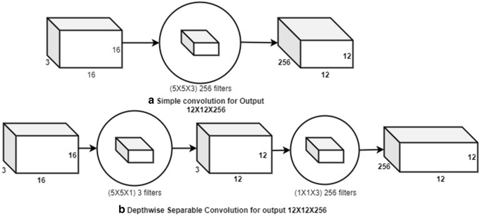
a Simple convolution for output 12 × 12 × 256 and b depthwise separable convolution for output 12 × 12 × 256

-
Input image size, N = 16 × 16 × 3
-
Size of the filter, f = 5 × 5×3
-
Stride, s = 1,
-
Padding, p = 0
-
Number of filters, n = 256
-
So output size, o = 12 × 12 × 3
-
256 filters will move for 12 × 12 times; hence, the number of multiplications required is:
When for the same instance, depthwise separable convolution is implemented as shown in Fig. 3b, number of multiplications required for such convolution can be computed as:
Step 1:
-
Input image size, N = 16 × 16 × 3
-
Size of the filter, f = 5 × 5×1
-
Stride, s = 1,
-
Padding, p = 0
-
Number of filters, n = 3
-
So output size, o = 12 × 12 × 3
-
3 filters will move for 12 × 12 times; hence, the number of multiplications required is:
Step 2:
-
Input image size, N = 12 × 12 × 3
-
Size of the filter, f = 1 × 1×3
-
Stride, s = 1,
-
Padding, p = 0
-
Number of filters, n = 256
-
So output size, o = 12 × 12 × 256
-
256 filters will move for 12 × 12 times; hence, the number of multiplications required is:
So the total multiplications required to perform the same task as shown in Fig. 3a using the separation shown in Fig. 3b are:
Hence, the computation for this example is reduced from 2,764,800 to 121,392, (as shown in Eqs. 1 and 4), which is approximately 22 times reduction, thereby giving the same result.
-
Global Average Pooling: This pools the average value of a feature map obtained after the convolution operations. It reduces the parameters to a large extent as compared to when using fully connected layers and thus avoids overfitting which may have occurred due to huge parameter learning.
-
Down sample the image size late in the network to extract more information: down sample the images gradually so that most of the relevant features are extracted out for better accuracy.
The network architecture build is shown in Fig. 2, which has 20 layers including 1 × 1 convolution, ReLU, pooling, batch normalization, depthwise separable convolution and global average pooling. Many variations in this network were built before finalizing on this architecture and trade-off was calculated between accuracy achieved and parameters required to be trained (or which is directly proportional to computation cost or memory requirement for the network). Each time the built network was trained on an NVIDIA GeForce GTX 680 GPU Server to perform exhaustive hyperparameter search. The final model took 8 h of training to stabilize on the loss and the accuracy. The network is trained on FER 2013 dataset and then robustly tested on different datasets including different backgrounds, different levels of emotions recorded spontaneous and posed which have different categories of people across the globe.
4.4 Reduction comparison in complexity order
As discussed in [34], authors have compared time complexity of different variants of convolutional neural network. The time complexity of all the convolutional layers in a network is:
Here \(n_{l - 1}\) is the number of filters in (l–1)th layer, \(s_{l}\) the length of the filter (3 for 3 × 3 filter size), \(n_{l}\) the number of filters in the lth layer, \(m_{l}\) the spatial size of the output feature map.
Based on this formula, we will be computing complexity for convolution operation, as classification part is kept same to avoid complexity in analysis. To further simplify this comparison, other parameters like pooling operation, batch normalization, etc., are kept same or checked if they are nullifying the complexity in the two models; hence, they are avoided. Also, considering the theoretical complexity, feature map size ml is temporarily omitted [34], hence computing it as
Also training time per image is three times its test time, as we have one forward propagation for testing and two extra backward propagations for training.
4.4.1 Time complexity for Vanilla CNN model
This model has 9 layers of convolution operation with batch normalization and ReLU activation function with each. Using each of the layers inputted and outputted number of filters, its time complexity (T(n)) is:
4.4.2 Time complexity of our proposed model
Our model has 10 layers of convolution operation as shown in Fig. 2 (architecture). The convolution operations here are consisting of 1 × 1 filters for three times, 3 × 3 filters for seven times. Time complexity (T(n′)) is computed below using the number of filters inputted and outputted to each layer.
Time complexity of our network is reduced to more than half of Vanilla CNN model that too when classification part was not considered. When fully connected layers are used in Vanilla CNN model, that would further increase its complexity to many folds. Hence, computationwise our model outperforms to be able to implement in real-time application like humanoid robots predicting human emotion.
5 Results
The network obtained for emotion recognition is robust in nature, works at a real-time speed and can be incorporated in real world. The loss obtained by the model is around 0.712 as shown in Fig. 4. Figure 5 shows the validation accuracy of the model which stabilizes to 74%. The accuracy obtained is improved over the state-of-the-art work carried out so far with reduced parameters to an extent of 50% as compared to the latest research to the best of our knowledge. This improvement in the accuracy is obtained by varying filter size, network convolution layers, down sampling the image size late in the network, so that the network can extract the best features over deep layers.

Loss plot of the network achieved while training the model. Here y-axis shows the loss and x-axis is the number of iterations

Validation accuracy of the network obtained while training the model. Here y-axis shows the accuracy on the validation data and x-axis is the number of iterations
Also using different datasets provides robustness to the network as all the possible variations are encountered by the network, like non-face image, illumination, age, occlusion, makeup, different backgrounds, Asian faces, black faces, Latino and white male and female variations.
Once the network was tested over all the above-mentioned datasets, confusion matrix for JAFFE dataset is shown in Fig. 6. As we can see from the table, most of the false predictions are in disgust emotion where disgust is mostly predicted as sad or sometimes neutral which is pretty much similar to human prediction as well. The second largest false predictions are in neutral face of JAFFE dataset where neutral is predicted as sad, surprise and sometimes fear which can be justified by the fact that the network here is dealing with Japanese faces.

Normalized confusion matrix for JAFFE dataset using the Vanilla CNN model is shown. Accuracy obtained for each emotion is mentioned in the diagonal entries; thereby, the average accuracy is 41.14%
Few images of dataset FER2013 are shown in Fig. 7. It shows variants in faces with different age groups, light effects, angles of the face. The dataset contains all the types of faces and even non-face images so that the network can generalize well.

Few samples from FER2013 dataset, showing that it contains all variants in the images, even images with no face (the first image in the second row)
Figure 8 shows the result of few images from JAFFE dataset with true positives and false positives expressions predicted. And Fig. 9 shows the result of images from custom dataset with the predicted labels. Network detects the faces from the group images and predicts the emotion for each face.

Test results on JAFFE dataset, out of which the first image in the second row is false prediction

Results from our custom dataset predicting the emotion in group images
Individual accuracy obtained for each emotion using Vanilla CNN, baseline model and our proposed model is shown in Figs. 6, 10 and 11, respectively. Figures 6 and 10 clearly show it lacks in prediction of angry and disgust emotion and less accuracy for other emotions as compared to Fig. 11 for our proposed model. Figure 11 shows highest accuracy obtained in sad emotion which is 86.67% and lowest is with fear emotion which is 46.67%. Average accuracy on JAFFE dataset (entirely new for the network) is 64.32%.

Normalized confusion matrix for JAFFE dataset using baseline model is shown. Accuracy obtained for each emotion is mentioned in the diagonal entries; thereby, the average accuracy is 61.85%

Normalized confusion matrix for JAFFE dataset using the Vanilla CNN model is shown. Accuracy obtained for each emotion is mentioned in the diagonal entries; thereby, the average accuracy is 64.32%
Improvement in the performance on our proposed network as compared to Vanilla convolution neural network and baseline model proposed in [20] is shown in Fig. 12. It shows the bar graph of accuracy value for each emotion using all the three models, and this indicates our model outperforms the benchmark model and also Vanilla CNN to be implemented on real-time systems. As shown in the bar graph, no successful prediction was found for angry and disgust emotion for other two methods. Also for other emotions, our model outperforms the baseline and Vanilla CNN models.

Comparison bar chart for three models is shown
6 Summary
The need for robot to understand human emotion is increasing with the increase in human–robot interaction. Robots, especially humanoid robots, and among them the personal humanoid robots, require to be more social in order to know the human sentiment and hence can gain confidence of the person to whom the robot is talking. When robot knows the human emotion, robots can customize the conversation ahead, in a better way. So here we are summarizing our research.
6.1 Conclusion
Real-time robust emotion classifier is built by reducing computational cost and achieving near human accuracy. This model built required 146,000 parameters and took 8 h’ time for getting trained to an accuracy of 65% on training and 74% on validation. Robustness of the model was verified over 8 datasets for emotions. Personal robots can be made more familiar after incorporating such emotion classifier and hence can be made more customized to the user. Through the sentiments, the person can stay more connected to the robot, and hence, the therapy, treatment to person via robots, will be more realistic.
6.2 Future work
The parameter requirement, memory requirement and hence the computation cost are reduced in our proposed method. In future, we will be integrating the same with NaO robot which is a humanoid robot. Such robots can be made more social when they will react in a realistic manner with the person.
Further, future work may include integrating more emotions which a human can understand. Now many mixed emotions are also being created which are just a merger of two existing standard emotions; for example, “happily surprised” and “fearfully surprised” can be further distinguished in order to make the conversation more realistic and customized.
References
Goodfellow IJ, et al. (2013) Challenges in representation learning: a report on three machine learning contests. arXiv e-prints
Wu X, Bartram L (2018) Social robots for people with developmental disabilities: a user study on design features of a graphical user interface. arXiv e-prints
Jaiswal S, Mishra P, Nandi GC (2018) Deep learning based command pointing direction estimation using a single RGB Camera. In: 2018 5th IEEE Uttar Pradesh section international conference on electrical. Electronics and Computer Engineering (UPCON)
Szegedy C, et al. (2014) Going deeper with convolutions. arXiv e-prints
Semwal VB et al (2017) Robust and accurate feature selection for humanoid push recovery and classification: deep learning approach. Neural Comput Appl 28(3):565–574
Chen L, Zhou C, Shen L (2012) Facial expression recognition based on SVM in E-learning. IERI Procedia 2:781–787
Chen X, et al. (2017) Convolution neural network for automatic facial expression recognition. In: 2017 International conference on applied system innovation (ICASI)
Alizadeh S, Fazel A (2017) Convolutional neural networks for facial expression recognition. arXiv e-prints
Ren X, et al. (2016) Convolutional neural network based on principal component analysis initialization for image classification. In: 2016 IEEE first international conference on data science in cyberspace (DSC)
Song T, Zheng W, Song P, Cui Z (2018) EEG emotion recognition using dynamical graph convolutional neural networks. IEEE Trans Affect Comput. https://doi.org/10.1109/TAFFC.2018.2817622
Samara A, Menezes MLR, Galway L (2016) Feature extraction for emotion recognition and modelling using neurophysiological data. In: 2016 15th international conference on ubiquitous computing and communications and 2016 international symposium on cyberspace and security (IUCC-CSS)
Lopes AT et al (2017) Facial expression recognition with convolutional neural networks: coping with few data and the training sample order. Pattern Recogn 61:610–628
Bawa VS, Kumar V (2018) Emotional sentiment analysis for a group of people based on transfer learning with a multi-modal system. Neural Comput Appl. https://doi.org/10.1007/s00521-018-3867-5
Mohammadpour M, et al. (2017) Facial emotion recognition using deep convolutional networks. In: 2017 IEEE 4th international conference on knowledge-based engineering and innovation (KBEI)
Anwar I, Islam NU (2017) Learned features are better for ethnicity classification. arXiv e-prints
Dachapally PR (2017) Facial emotion detection using convolutional neural networks and representational autoencoder units. arXiv e-prints
Tripathi S, et al. (2017) Using deep and convolutional neural networks for accurate emotion classification on DEAP dataset. 2017
Pilla V, Zanellato A, Bortolini C, Gamba HR, Borba GB, Medeiros H (2016) Facial expression classification using convolutional neural network and support vector machine. In: Conference proceedings
Ko BC (2018) A brief review of facial emotion recognition based on visual information. Sensors, 2018. In: Conference proceedings
Arriaga O, Valdenegro-Toro M, Plöger P (2017) Real-time convolutional neural networks for emotion and gender classification. arXiv e-prints
Iqbal MTB, Wadud MA, Ryu B, Makhmudkhujaev F, Chae O (2018) Facial expression recognition with neighborhood-aware edge directional pattern (NEDP). IEEE Trans Affect Comput. https://doi.org/10.1109/TAFFC.2018.2829707
Dibeklioglu H, Gevers T (2018) Automatic estimation of taste liking through facial expression dynamics. IEEE Trans Affect Comput. https://doi.org/10.1109/TAFFC.2018.2832044
Al Chanti DA, Caplier A (2018) Deep learning for spatio-temporal modeling of dynamic spontaneous emotions. IEEE Trans Affect Comput. https://doi.org/10.1109/TAFFC.2018.2873600
Ding S et al (2017) Extreme learning machine with kernel model based on deep learning. Neural Comput Appl 28(8):1975–1984
Williams RJ, Zipser D (1989) A learning algorithm for continually running fully recurrent neural networks. Neural Comput 1(2):270–280
Pierre-Luc Carrier AC (2013) Challenges in representation learning: facial expression recognition challenge
Lucey P, et al. (2010) The extended Cohn-Kanade dataset (CK +): a complete dataset for action unit and emotion-specified expression. In: 2010 IEEE computer society conference on computer vision and pattern recognition—workshops
Ma C (2015) Wittenbrink, The Chicago face database: a free stimulus set of faces and norming data. Behav Res Methods 1122–1135:47
Lyons MJ, Akamatsu S, Kamachi M, Gyoba J (1998) Coding facial expressions with gabor wavelets. In: 3rd IEEE international conference on automatic face and gesture recognition, 200–205
Thomaz CE FEI face database
Setty S, et al. (2013) Indian movie face database: A benchmark for face recognition under wide variations. In: 2013 fourth national conference on computer vision, pattern recognition, image processing and graphics (NCVPRIPG)
Li-Fen C, Taiwanese Y-SY (2007) Facial expression image database. Brain Mapping Laboratory, Institute of Brain Science, National Yang-Ming University, Taipei, Taiwan
Wang C-F (2018) A basic introduction to separable convolutions
He K, Sun J (2015) Convolutional neural networks at constrained time cost. In: CVPR
Acknowledgement
We are highly grateful to all our laboratory members for providing their consent for photographs for our custom dataset. Thanks to all the emotion dataset providers over internet which we have used in our project.
Author information
Authors and Affiliations
Corresponding author
Ethics declarations
Conflict of interest
The authors declare that they have no conflict of interest.
Additional information
Publisher's Note
Springer Nature remains neutral with regard to jurisdictional claims in published maps and institutional affiliations.
Rights and permissions
About this article

Cite this article
Jaiswal, S., Nandi, G.C. Robust real-time emotion detection system using CNN architecture. Neural Comput & Applic 32, 11253–11262 (2020). https://doi.org/10.1007/s00521-019-04564-4
Received:
Accepted:
Published:
Issue Date:
DOI: https://doi.org/10.1007/s00521-019-04564-4