Abstract
Nowadays, skin cancer is considered a serious disorder in which early identification and treatment of the disease are essential to ensure the stability of the patients. Several existing skin cancer detection methods are introduced by employing deep learning (DL) to perform skin disease classification. Convolutional neural networks (CNNs) can classify melanoma skin cancer images. But, it suffers from an overfitting problem. Therefore, to overcome this problem and to classify both benign and malignant tumors efficiently, the multi-stage faster RCNN-based iSPLInception (MFRCNN-iSPLI) method is proposed. Then, the test dataset is used for evaluating the proposed model performance. The faster RCNN is employed directly to perform image classification. This may heavily raise computation time and network complications. So, the iSPLInception model is applied in the multi-stage classification. In this, the iSPLInception model is formulated using the Inception-ResNet design. For candidate box deletion, the prairie dog optimization algorithm is utilized. We have utilized two skin disease datasets, namely, ISIC 2019 Skin lesion image classification and the HAM10000 dataset for conducting experimental results. The methods’ accuracy, precision, recall, and F1 score values are calculated, and the results are compared with the existing methods such as CNN, hybrid DL, Inception v3, and VGG19. With 95.82% accuracy, 96.85% precision, 96.52% recall, and 0.95% F1 score values, the output analysis of each measure verified the prediction and classification effectiveness of the method.
Keywords: Skin cancer prediction, Prairie dog optimization, Intelligent signal processing lab inception, Region proposal networks
Introduction
The growth of abnormal cells in the body leads to the generation of skin cancer, further depending upon their features, nature, and seriousness may spread to various organs of the human body. The visible part obtained in the human body is the skin which is easily affected by environmental infections, and this leads to generating skin cancer. Each year 46,000 new people were affected by skin cancer in the UK. Melanoma and non-melanoma are the types of skin cancer. Non-melanoma is divided into two types that are basal cell skin cancer (BCC) and squamous cell skin cancer (SCC). The melanoma type is lethal [1]. Melanoma-type skin cancer is caused by a variety of factors such as the radiation of ultraviolet (UV) and genetic aspects. Melanoma starts from skin melanocytes and which yield dark pigment on the body [2]. BCC and SCC perform metastasize infrequently. So, they have a low level of risk and it causes a low-level death rate. But the occurrence of non-melanoma type is rare. In 2017, WHO reports two to three million people were affected by non-melanoma [3]. Skin cancer melanoma is complex, so early identification of this type is most important because of the decreasing death rate and also supports saving the patient’s life. The visual image of melanoma and non-melanoma is the same. So, identification of which type of skin cancer occurs is a challenging work which is why the lesion representation for the successful classification of lesions is developed [4].
To detect skin cancer, various methods are there. To obtain the skin images on the lesion, the Dermatoscope device is used. The technique of classification of dermoscopy image is used to identify the issues and mainly to identify the boundary characteristics, to measure the shape of the lesion [5]. Artificial intelligence (AI) and machine learning (ML) algorithms are best to detect skin can cancer accurately and also better for hospital decisions. However, in UK, AI/ML algorithms are currently not used for detecting doubtful skin lesions. There is a variety of reasons, but one of the most things is the need for powerful evidence. The CanTest framework established the new diagnostic tests and the clinical training and offered guideline developers and rule makers to connect from development to implementation [6]. The CNN and the physicians classified the skin lesion of dermoscopic images into five categories than the relevant skin cancer. This approach independently detects each other. Then, the result will be merged with all classifiers. Ninety percent of lesions were found in this examination. If any errors will be occurring, both systems were related weakly [7]. To identify the classification of multi-class skin cancer, the CNN classifier was used, which used four groups of methods for the best classification on the dataset, namely, HAM10000. Transfer learning was performed to learn the features of the skin cancers in the particular domain and did not consider the lesion parts to generate the work common.
The DL approach is more effective for large inputs [8–12]. It is based on the computerized diagnosis. This approach is employed in feature extraction and fusion. The ABCDE approach also detects skin cancer through lesion classification. The features should be extracted correctly to detect skin cancer automatically and also extract the features from the correct lesion parts [13]. The ABCDE rule identifies the general sign of melanoma such as irregularity, asymmetry, multi-color, and dermoscopic structure. The ABCDE rule performs three stages. First, detect and remove the hair and generate the skin lesion to be clearly visible and then color normalization will be performed [14]. For skin cancer target detection, the CNN-based target detection technique is introduced. Faster RCNN is chosen as the default detection network due to its high detection speed and accuracy. The traditional model relies on features and pixels. The pixel-based detection method is used to identify the target by determining if each pixel’s level of gray exceeds a predetermined threshold. The lack of an accurate model, the high rate of false alarms, and the difficulty in threshold selection are the limitations of the skin cancer detection approach [15].
The growth of skin cancer melanoma is generated deeper into the skin, and the delay in diagnosis leads to reaching severity level as well as spreading to other parts of the body. It is complex to treat skin cancer when spread to other parts. The non-invasive technique called dermoscopy is obtained for treating skin cancer by oil immersion and incident light which makes visualization of the skin surface. The dermoscopy diagnosis of skin cancer depends on training the dermatologist. Hence, the diagnosis of skin cancer in an automated way is significant for less-experienced physicians. The automatic detection of skin cancer restricts the segmentation process by utilizing texture analysis. Texture analysis is highly applicable for the automatic detection of skin cancer. The texture measures are determined by gray-level co-occurrence matrix (GLCM) [16]. In this paper, a modified faster RCNN model is proposed for skin cancer prediction. The algorithm lays the base for additional skin cancer real-time status detection by concurrently increasing computational accuracy and operation speed. The faster RCNN and iSPLInception algorithm-based two-stage classification model is then developed. The main contribution of the paper is described below:
The faster RCNN is mainly selected as the base detection network due to its higher detection speed and accuracy. The faster RCNN is integrated with the iSPLInception model to prevent it from overfitting the features.
The skin lesion information is identified using the region proposal network (RPN) of the faster RCNN model. In this way, the operation speed and computational accuracy are improved to support real-time skin cancer prediction.
The faster RCNN and the iSPLInception form a two-stage classification model where the skin cancer features such as border, color, diameter, and asymmetry are extracted by the faster RCNN architecture to differentiate between the normal and abnormal classes. The iSPLInception improves the classification accuracy of the proposed model.
The accuracy of the proposed approach is proven to be superior to traditional methods, and the efficiency is determined in analyses of the result.
Related Works
For early prediction of skin cancer, Zhang et al. [2] presented optimized CNN. The Whale Optimization algorithm is used to optimize the developed CNN. It determines the difference obtained between the network and desired output. Performance metrics specificity, accuracy, and sensitivity were used to evaluate the result but CNN required more training data for effective results. Imran et al. [17] introduced the ensemble of deep learners for predicting skin cancer. The three deep learning models VGG, Caps-Net, and ResNet were utilized to develop it. An ISIC dataset was used for getting input images. The ensemble had a 106-s categorization training time and a 93.5% average accuracy. The established method enhanced the performance but ResNet required more training time.
Maniraj and Maran [18] developed a hybrid deep learning (HDL) in skin cancer detection. Unnecessary information, including nose and hair, was eliminated using a simple median filter. The developed method was used to conduct multi-class classification utilizing the fused subband, but it needed more computational time. A CNN stacked ensemble framework was presented by Shorfuzzaman [19] for the early detection of melanoma skin cancer. The transfer learning concept was obtained to classify the skin cancer types (i.e., malignant or benign). However, this model was unable to make use of the segmented melanoma images created by segmentation networks.
Narunsky-Hazzia et al. [20] utilized cancer-type-specific fungal ecologies bacteriome interaction for pan-cancer analyses. The illustrated model analyzed the characteristics of cancer mycobiome within 17,401 patient tissue, blood, and plasma samples. The established model developed prognostic and diagnostic capacities of tissue and plasma microbiomes, in stage 1. On the other hand, the analyzed model only focuses on the fungal kingdom and does not focus on any real-world data which supports increasing the accuracy of the classification. Kausar et al. [21] utilized to categorize multi-class skin cancer using a deep learning–based ensemble model. The performance was validated by CNN and attained 98% and 98.6% accuracy when evaluating deep learning–based ensembles. Meanwhile, the majority of the skin cancer classification was not included in this approach.
Sripada and Mohammed [22] utilized a deep CNN model to predict and classify multi-class skin cancer. This model has differences in the skin lesion between squamous cell carcinoma, basal cell carcinoma, and malignant melanoma. This model offers an accuracy value of 97.156% when evaluating dermoscopic images. However, this model does not improve the medical image in the image processing system. Ali et al. [23] utilized a multi-class skin cancer classification by efficient Nets for preventing skin illustrated model. Analyze the influence of transfer learning on pre-trained weights of Image Net variants on an imbalanced multi-class classification problem. This model offers accuracy, precision, recall, accuracy, and F1 score when evaluated at HAM10000. The experimentation results reviewed that the established method attained a superior performance when compared with the existing method. On the other hand, the method did not include any real-world data which supports increasing the accuracy of classification.
Proposed Model
Faster RCNN
An excellent work in the field of target detection is the faster RCNN algorithm [24]. The convolution network is the RPN which the input images are prognosticated based on the position of every candidate box. The RPN network is a determined alternative to the conventional selective search approach; it essentially eliminates the time overhead associated with candidate region selection.
Loss Function
The mathematical expression for the loss function is:
| 1 |
where j represents an anchor’s index in this mini-batch. is the target’s anchor’s prediction probability.
| 2 |
The classification loss function is given as:
| 3 |
The offset detected by this anchor is represented by the vector . The actual offset of the ground-truth box is represented by , which is a vector of the same dimension as . The box regression loss function can be stated as:
| 4 |
the function is represented by the term W:
| 5 |
The adversarial network is denoted as B (M), and the original target detection network is shown as A (M). Where M stands for the candidate region for B, assume that C is B’s actual category. The adversarial network’s loss function can be written as:
| 6 |
Region Proposal Networks (RPNs)
Instead of conducting a select search, the sliding window mechanism is utilized to create the region for the RPN candidate [25]. An eigenvector in 256 dimensions is provided to the layer of the convolution feature in which the median portion is determined as an anchor. At each position, the anchor boxes are obtained. The scores are then utilized to determine whether the candidate region contains detection targets, and throughout 2 full connections, 2 scores are obtained by one connection and 4 scores by the other connection. The potential region’s coordinates, including its width and length. The coordinates of the central position. The network’s output performance can be impacted by the configuration of the size, width, and length.
| 7 |
| 8 |
| 9 |
From the above equation, the loss equation is denoted as generated by regression and classification of bounding boxes and .
In the above equation, the loss function is denoted by where is smooth and derived using the below equation.
| 10 |
Both and are normalized weight parameters that represent how many anchor positions are obtained in total and then determine the input in the low image. The sample label is denoted by , the probability that the anchor box contains the target is represented by . The mathematical equation for and , the real and predicted bounding box coordinates is shown in the below equation.
| 11 |
where , , and are the predicted candidate, and real target bounding box coordinate.
Prairie Dog Optimization
The prairie dog spends most of its days feeding, watching out for predators, digging new burrows, or maintaining those that already exist [26]. The behavior of animals based on AI is focused on disease monitoring, processing, and growth estimation. In AI the cost and the accuracy are enhanced. The behavior of each individual is operated by the function of the brain and the animal behavior is validated by AI for providing an appropriate response to disease.
Initialization
Each prairie dog (PD) in a coterie is a member of one of the m coteries. The position of a jth prairie dog inside a specific coterie can be determined by a vector because PD exists and work as a coterie or unit. The entire coteries (C) location present in the colony is described in the below equation.
| 12 |
Here, depicted the colony’s coterie's dimension. The entire prairie dog position in the coterie is described in the below equation:
| 13 |
From the above equation, where is the prairie dog in a coterie’s dimension, and . Utilizing the below uniform distribution equation, the position of the prairie dog and each coterie is assigned:
| 14 |
| 15 |
The dimensions upper and lower bound in the optimization issue is represented as and , the uniform distribution in the range (0,1), and its random number is depicted as and , and
Evaluation of Fitness Function
The solution vector is fed into the specified fitness function to determine the value of the fitness function for each position of the prairie dog. The below array present in Eq. 16 saved the outcomes.
| 16 |
The food quality available at a certain source, the capacity to dig new burrows, and the ability to react appropriately to anti-predation alarms are all described by the fitness function values for each prairie dog. The fitness function values are stored in an array that is sorted, and the minimal fitness value that is received is deemed the best answer thus far to the specified minimization problem. The following three are taken into account along with the best value when creating burrows to aid in predator avoidance.
Exploration
The PDO exploratory process is explained in this section. Based on four criteria, the PDO might choose between exploration and exploitation. The maximum iteration number is separated into four equal sections, with the exploration taking up the first two and the exploitation taking up the final two. For exploitation, we utilized two tactics based on and . For exploration, we utilized two tactics based on and .
They produce characteristic noises to alert other individuals of the discovery of food sources. In accordance with the food source quality, the best is accessed, chosen for foraging, and new burrows are constructed. In the stage of exploration, the position upgraded for foraging is expressed in Eq. 17. The second tactic is to examine the strength of the digging and the quality of the available food sources. Depending on the concept that digging strength will decrease as the iteration number rises, new burrows are constructed. This circumstance aids in limiting the potential number of burrows. For the building burrow, the position is upgraded in Eq. 18
| 17 |
| 18 |
The global best-obtained solution is represented as . The effect of the most recent best solution, as given in Eq. 19, is evaluated by , The experiment’s specialized food source alarm, , is set to 0.1 kHz. The random solution position is depicted as . Equation 20 defines as the randomized cumulative effect of entire prairie dog present in the colony. The strength of the coterie’s digging, denoted by , is determined by the characteristic of the food source and has a random value determined by Eq. 21.
| 19 |
| 20 |
| 21 |
Here, the stochastic property is introduced to assure exploration. Although the PDO implementation was based on the assumption that all prairie dogs were the same, represents a tiny number that accommodates variations in the prairie dogs.
Exploitation
The PDO exploitation behavior is explained in this section. These two distinct behaviors cause the prairie dogs to congregate at a particular position or determine an extra exploitation phase to evaluate the optimal solution. In the case of PDO implementation, a prospective position, where additional search (exploitation) is conducted to identify optimal solutions nearly. The purpose of the PDO’s exploitation mechanisms is to thoroughly seek the promising areas discovered throughout the phase of exploration. As mentioned in the previous section, the PDO travels between two tactics, namely and , to balance its exploration and exploitation behaviors.. The two approaches Eqs. 22 and 23 are models that have been adopted for this phase.
| 22 |
| 23 |
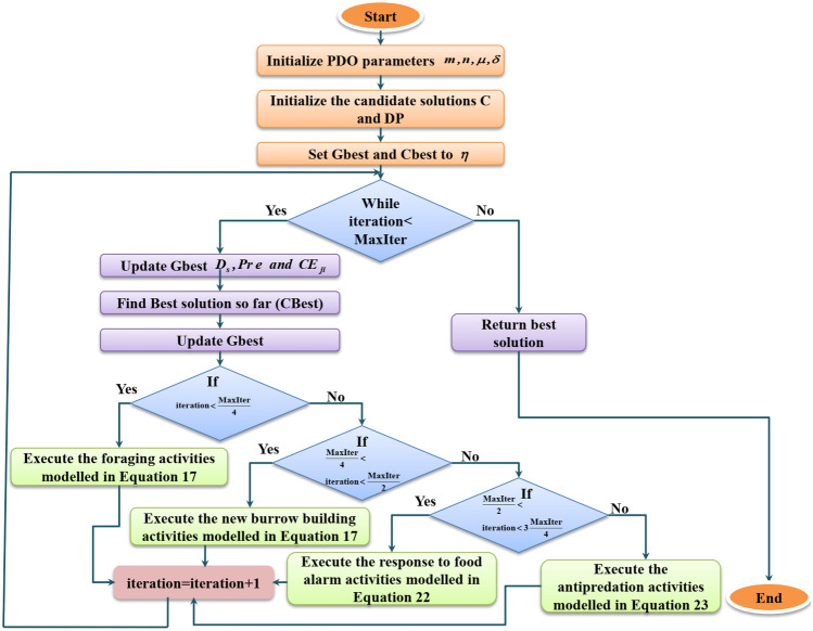
The global best-obtained solution is represented as . The effect of the most recent best solution, as given in Eq. 19, is evaluated by , the source of food quality described . The entire prairie dog cumulative effect in the colony is expressed as . The predator effect is represented as the number lying in the interval [0, 1]. Figure 1 depicts the flowchart for PDO algorithm.
| 24 |
Fig. 1.
PDO algorithm flowchart
RPN Optimization
The ratio of skin disease lesions to images does not change when lesion positioning is done utilizing skin cancer detection images. As opposed to conventional target identification issues, there is no need to create many anchor boxes at each anchor point that is of various sizes, and when RPN is used to select candidate regions, ratios are at each anchor point. The skin disease lesion distribution information and location in the image can be utilized to optimize the anchor boxes’ ratios, overlaps, and sizes. Here, relative coordinates rather than absolute ones are used to optimize the anchor box scale because the image’s size and skin disease lesions vary with scaling ratios and acquisition parameters.
Assume that the training data set contains skin disease features that have been labeled, and that the skin lesion’s candidate region has coordinates for its width , center , and length . and are the image’s overall width and length. The ratio of length to width and relative scale is defined as follows because they are consistent for both images and lesions.
| 25 |
| 26 |
Overlaps could occur when creating candidate boxes. Here, for candidate box deletion, the prairie dog optimization algorithm is utilized. Here, 0 is chosen as the threshold value because for practical lesions there is no overlap, and the computation process is given below.
Phase 1: The candidate box employing the best rating should be selected.
Phase 2: The intersection of the union’s (IOUs) value between the one selected in phase (1) and each of the remaining boxes should be evaluated. The related candidate box is eliminated and considered invalid if the threshold value is higher than the predetermined.
Phase 3: Phases (1) and (2) given above are repeated until there are no more candidate boxes to remove, and among the boxes that have not been deleted yet, pick the one with the best score is continued.
To speed up model optimization in the experiment, the adaptive vectors are utilized to validate the updating rate and best performance. 0.001 is chosen as the starting point. The current model’s precision and loss are assessed in the validation set after each training epoch. Every other epoch shows the changes in loss value when they are less than 0.0001. The following equation is used to modify the learning rate.
| 27 |
The adjustment coefficient is denoted by gamma and the gamma value is 0.1.
A Model of Intelligent Signal Processing Lab Inception (iSPLInception)
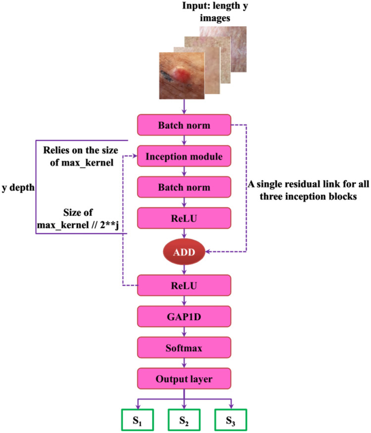
The performance of skin cancer detection (SCD) systems is enhanced by the earlier DL methods, but the overfitting problem is not solved properly [27]. To focus on the process of SCD, based on the Inception-ResNet design, the iSPLInception model is designed. Particularly, the inception block and residual link of the Inception-ResNet design are considered. When constructing extremely wide and deep models, the inception blocks were mostly helpful. The convolutions containing different sizes of a kernel are operated parallel within every inception block, and then those parallel processes provided outputs are combined. Here, the input is returned by the instant preceding layer of this inception module. It is linked with the max pooling function (MaxPool1D) and the Conv1D (1D convolution layer). For the input characteristics, the dimensionality reduction layer is operated by the Conv1D which is an inexpensive process. Input channels are decreased to one by the Conv1D, and for the three convolution layers (, , Conv1D), it serves as the input. The hyperparameter of max_kernel size establishes and Conv1D layers’ kernel size. With the Conv1D layer, the layer of Maxpool1D is linked, which is then linked with the concatenation layer or residual node.
The architecture of iSPLInception is depicted in Fig. 2. A set of images of even length, i.e., the size of the window, is the input for the SCD issue. (Size of window, number of images, batch size) is the input sequence format. R defines the number of samples in the input array which is expressed below:
| 28 |
Fig. 2.
Architecture of iSPLInception
The spatial frequency is represented as is expressed in cycles per meter, and every window size is . Here, based on the utilized dataset, the size of the window changes. The BatchNorm layer (Batch normalization) gets these input images, and it performs like the preceding layer of the 1st inception module. Then, before rectified linear unit (ReLU), the inception block produced output is taken by the next BatchNorm layer. The depth hyperparameter decides the number of ReLU layers, BatchNorm, and inception block. Without raising the size of the model concerning parameters, this iSPLInception model can be made deeper and wider by adding several inception modules. The BatchNorm layer is connected to the activation layer output using the add layer by establishing one residual link to all three modules.
The ReLU activation layer activates the residual function’s output. The model’s depth hyperparameter determines the residual link’s existence. Whether or not the residual link is present in the inception block is verified by the 2nd ReLU activation to activate. A shortcut is formed by using the residual link, and the new data can be given to subsequent layers via the skip link. A large amount of data can also be learned by the subsequent layers like the previous layers from similar input data. The GAP1D (1-D Global Average Pooling) module is placed after the last ReLU activation layer. Here, the ReLU provided output passes via GAP1D.
Classification Layer
For the HAM10000 dataset, a categorical cross-entropy (CE)-based Softmax classifier is utilized, and for ISIC 2019 dataset, a binary CE-based sigmoid classifier is utilized. Normally, the expression for cross-entropy loss is given by:
| 29 |
For class within classes, the predicted values (model scores) and actual values are represented as and . Prior to evaluating the CE loss, the activation functions such as Sigmoid or Softmax are used for scores. Hence, the activations can be denoted using . The binary classification difficulty arises when working on ISIC 2019 dataset. So, an activation function of the sigmoid is employed, which divides the input vector within intervals, and it was used separately toward each component of scores ,. The below equation describes the activation function of the sigmoid as:
| 30 |
For input , the sigmoid function is denoted as , and Euler’s number is represented as . Binary CE loss for a sigmoid function is acquired by integrating Eqs. (29) and (30). It is expressed as:
| 31 |
| 32 |
In addition, an activation function of Softmax is employed, which divides the input vector within the interval. Then, every resultant component is added together to form one. Since the Softmax function relies on every vector element, it does not be calculated separately for every input value. Softmax function converts the input values such as negative, positive, > 1, or zero into values from 0 to 1. They can therefore be taken like probabilities. For every input vector, the model is trained to produce the probability within classes . For the input vector, the Softmax function is expressed as:
| 33 |
For an output and input vector, a standard exponential operation is referred to as and , and an input vector is indicated as . The normalization expression is defined by , which sums up the output values into one. Categorical CE loss for Softmax function is acquired by integrating Eqs. (29) and (33). It is expressed as:
| 34 |
For a positive class , the Softmax score is denoted as in the above equation. If there are one-hot encoded labels, then just a positive class maintains its loss expression in the classification of multi-class.
Proposed Multi-Stage Classification Approach Using Faster RCNN and iSPLI
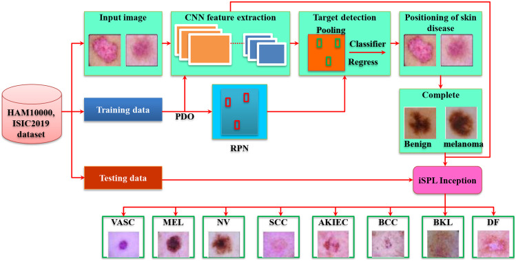
Faster RCNN gives the complete skin disease and its associated matches. The normal and abnormal classes of the entire skin disease are determined. During the application of a conventional multi-class classification algorithm for training, the dissimilarity between abnormal samples is more compared to the dissimilarity between abnormal samples and normal skin disease containing low-level divergence. This is mainly due to the changes in the dissimilarity levels for abnormal skin disease. The faster RCNN is employed directly to perform classification. This may heavily raise computation time and network complications. So, the iSPLInception model is applied in the multi-stage classification. Here, training utilizes the normal skin disease samples, and then the skin disease that is abnormal or normal is decided using the iSPLInception architecture. During the classification, abnormal skin diseases are observed when the decision condition does not fulfill. VASC, MEL, NV, SCC, AKIEC, BCC, BKL, and DF are the classification of abnormal skin diseases. Figure 3 depicts the architecture of the faster RCNN-iSPLInception model.
Fig. 3.
Faster RCNN-iSPLInception model
Preprocessing is the initial and essential step for restricting redundant data and removing noise. This scenario is applied in medical images for removing air bubbles, artifacts, and noise and enhances the datasets to obtain real images. The noises obtained in the images are removed to perform a superior classification of skin cancer types. The features of the images are extracted to classify malignant and benign types [28].
Once the process of training is completed, subsequently the faster RCNN created entire skin disease images are obtained to perform feature extraction of regional images. The changes in the skin disease image are efficiently indicated by the image histogram data. Therefore, feature extraction is executed with the help of histogram data. The below-mentioned equation is utilized for evaluating gray histogram data.
| 35 |
From the above equation denotes the pixel values, grayscale is indicated as , the highest gray scale value of an image is indicated as, and the total pixels within an image containing gray scale is represented as . To classify skin disease images, the iSPLInception model is applied. Then, for achieving the features of images, the normal skin disease images are processed initially within the training dataset. In the testing dataset, the image features that need to test are computed and given to the iSPLInception model. As a result, both the normal and abnormal skin cancer images are classified by this model.
Figure 4 depicts the flow chart for the proposed method with optimization methods. The images are considered as input and faster RCNN is obtained with ISIC 2019 and HAM10000 datasets for target detection. The RPN is determined by a sliding window mechanism to evaluate the candidate region based on the detection target. The regression and classification weight parameters are employed in RPN to validate the anchor positions. The overlapping of multiple images is controlled by the PDO approach and validated AI based on animal behavior. The features are extracted, and the images are classified to determine whether it is a benign or malignant stage.
Fig. 4.
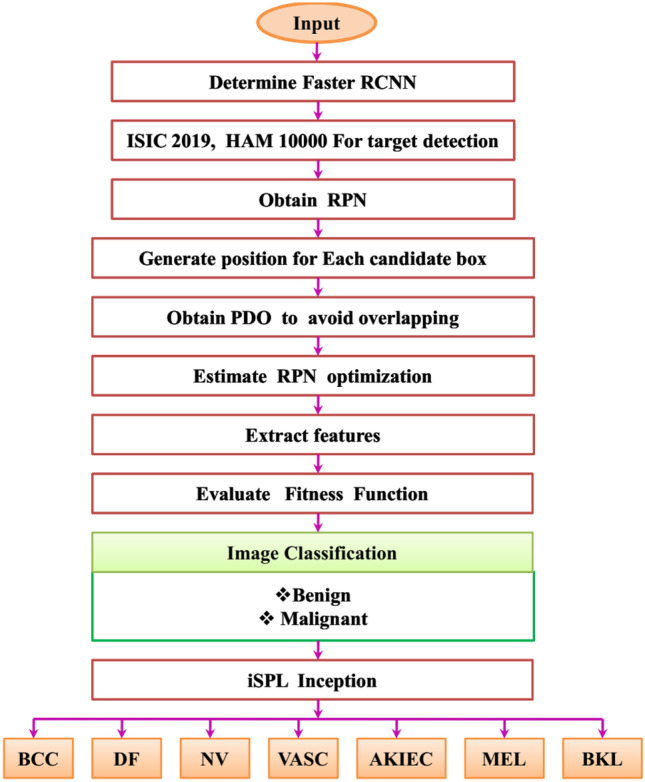
Flow chart of the proposed method
Results and Discussion
For tackling the challenges posed by the skin cancer diagnosis and classification model, this paper presents the MFCRNN-is PLI method. For proving the influence of the MFCRNN-isPLI method, two skin diseases datasets like the ISIC 2019 Skin lesion image dataset and the HAM10000 dataset were utilized. The accuracy of ISIC 2019, the HAM10000 dataset, and the speed of image processing have all somewhat improved when compared to another target identification system called faster RCNN. The network distributes the convolution elements when training is performed based on faster RCNN and RPN which significantly decreases the number of parameters required for training and increases training effectiveness. The four existing classification methods like optimized CNN HDL, Inception v3, and VGG19 were chosen for comparing the output values of accuracy, precision, recall, ROC, and F1 score values. The lesion identification model used in this study works on hardware that includes an Intel i7 9700 processor, NVIDIA RTX2080 GPU, and 32 GB of RAM. The performance of the proposed method is evaluated using Windows 10, Python 3.6, CUDA 9.0, Tensorflow, and Cuda Deep Neural Network (cuDNN) 7.3 software environments. In this paper’s training process, the number of iterations is arranged to 4000 times. To acquire the skin lesion detection result. The training images are obtained in the image dataset to determine the faster result.
Evaluation Measures
The ratio of precisely classified images and whole images is represented as accuracy. The effectiveness of the model is directly evaluated. The validity of the accuracy is justified when all the class distributions are simultaneous. The predicted classes should match the actual class for accurate prediction. The proportion of images precisely marked as the belongings of the positive class to the whole images marked under the positive class is called precision. The fraction of true positives precisely predicted using the model over the images belonging to the positive class amounts to the recall metric. Since the F1 score () is the trade-off between precision and recall, we might have to increase one over the other depending on the user requirements and application domain. The model’s higher classification power is shown by the higher F1 score values.
Dataset Description
ISIC 2019 Skin Lesion Images for Classification
It includes 25,331 dermoscopic images with nine various categories of cancer [29]. They are given as follows: basal cell carcinoma, melanoma, benign keratosis (solar lentigo/seborrheic keratosis/lichen planus-like keratosis), vascular lesion, squamous cell carcinoma, melanocytic nevus, dermatofibroma, actinic keratosis, and none of the above.
The HAM10000 Dataset
Factors such as lack of diversity and the small size of the dermatoscopic image dataset impact to detection of skin disease automatically in neural networks [30]. To tackle these issues, human against machine with 10,000 training images (HAM10000) dataset was utilized which was acquired from varied populations and stored using various modalities. It comprises 10,015 dermoscopic images for training. The various pigmented lesion diagnostic categories included in this dataset are basal cell carcinoma (bcc), dermatofibroma (df), melanocytic nevi (nv), vascular lesions (angiomas, angiokeratomas, and hemorrhage, vasc), actinic keratoses and intraepithelial carcinoma and Bowen’s disease (akiec), melanoma (mel), and benign keratosis-like lesions (solar lentigines and lichen-planus-like keratoses, bkl).
The training and testing are performed in the ratio of 80:20. The training of the image is performed with the HAM10000 dataset and testing with ISIC 2019 skin lesion image.
Table 1 depicts the number of images of two datasets ISIC 2019 and HAM 10000 and classified the images with training and testing mechanisms for evaluation. The images of training will be high compared to testing.
Table 1.
Dataset comparison
| Dataset | Number of images | Training | Testing |
|---|---|---|---|
| ISIC 2019 | 25,331 | 20,265 | 5,066 |
| HAM 10000 | 10,015 | 8,012 | 2,003 |
The comparison of ISIC 2019 and HAM 10000 datasets based on AKIEC, BCC, BKL, DF, MEL, NV, SCC, and VASC classes are delineated in Tables 2 and 3. These are evaluated by training, testing, and validation method. The total number of images determined for training, testing, and validation is 20,267, 2532, and 2532. The overall class images are determined by 25,331.
Table 2.
Different class comparison of the ISIC 2019 dataset
| Class | Training | Testing | Validation |
|---|---|---|---|
| AKIEC | 693 | 87 | 87 |
| BCC | 2659 | 332 | 332 |
| BKL | 2100 | 262 | 262 |
| DF | 191 | 24 | 24 |
| MEL | 3618 | 452 | 452 |
| NV | 10,301 | 1287 | 1287 |
| SCC | 502 | 63 | 63 |
| VASC | 203 | 25 | 25 |
| Total images | 20,267 | 2532 | 2532 |
| Overall images | 25,331 | ||
Table 3.
Comparison of various classes of the HAM 10000 dataset
| Class | Training | Testing | Validation |
|---|---|---|---|
| AKIEC | 261 | 33 | 33 |
| BCC | 412 | 51 | 51 |
| BKL | 879 | 110 | 110 |
| DF | 91 | 12 | 12 |
| MEL | 891 | 111 | 111 |
| NV | 5363 | 671 | 671 |
| VASC | 114 | 14 | 14 |
| Total images | 8011 | 1002 | 1002 |
| Overall images | 10,015 | ||
Comparative Analysis
The proposed MFCRNN-isPLI technique evaluates the accuracy of the optimized CNN, HDL, Inception v3, and VGG19 while validating with ISIC 2019 Skin Lesion images dataset. Among them, the MFCRNN-isPLI method has higher accuracy of 96.25% which is 25% higher than CNN, 29% higher than hybrid DL, and 19% higher than the Inception v3. Similarly, the proposed MFCRNN-isPLI method achieves higher accuracy while examining the HAM10000 dataset the accuracy attained by the proposed method is 95.74%. The gained accuracies of existing methods are as follows: CNN gained 88.52%, hybrid DL gained 84.31%, and Inception v3 gained 89.41%. Thus, the proposed MFCRNN-isPLI method has better performance in terms of accuracy in both datasets.
VGG19, Inception v3, CNN, and hybrid DL are the existing methods compared with the proposed MFCRNN-isPLI method. Our proposed method achieved high precision of 97.6% than the existing methods VGG19, Inception v3, CNN, and hybrid DL. For the HAM10000 dataset, the MFCRNN-isPLI method is compared with existing methods such as VGG19, Inception v3, CNN, and hybrid DL. Comparing existing methods, the proposed MFCRNN-isPLI method has high precision of 95.55%
The recall performance of the proposed MFCRNN-isPLI and existing methods utilizing the ISIC 2019 Skin Lesion images dataset and HAM10000 dataset. The MFCRNN-isPLI method has a recall value of 95.25%, and recall values of CNN, hybrid DL, and Inception v3 are 94.52%, 84.41%, and 86.51%, respectively. During training and evaluating with the HAM10000 dataset, the MFCRNN-isPLI method achieved a 97.52% recall value and CNN acquired a 90.25% recall value which is 15.25% lesser than the proposed method. The hybrid DL has 84.25% recall which is 22.52% lesser. Inception v3 and VGG19 acquired 83.52% and 89.31% accuracies.
Table 4 depicts the existing CNN, hybrid DL, Inception v3, VGG19, and the proposed MFCRNN-isPLI method comparison with ISIC 2019 skin lesion image and HAM10000 dataset. The comparison is performed with different parameter metrics for evaluating the performance.
Table 4.
Dataset comparison with different parameters for the proposed method
| Datasets | Methods | Accuracy (%) | Precision (%) | Recall (%) |
|---|---|---|---|---|
| ISIC 2019 skin lesion image | CNN | 87.32 | 86.82 | 94.52 |
| Hybrid DL | 84.91 | 94.54 | 84.41 | |
| Inception v3 | 89.93 | 86.72 | 86.51 | |
| VGG19 | 94.62 | 83.18 | 89.95 | |
| MFCRNN-isPLI | 96.25 | 97.6 | 95.25 | |
| HAM 10000 | CNN | 88.52 | 91.83 | 90.25 |
| Hybrid DL | 84.31 | 85.62 | 84.25 | |
| Inception v3 | 89.41 | 83.41 | 83.52 | |
| VGG19 | 91.45 | 87.48 | 89.31 | |
| MFCRNN-isPLI | 95.74 | 95.55 | 97.52 |
Table 5 summarizes the outputs of testing the proposed MFCRNN-isPLI, CNN, hybrid DL, Inception v3, and VGG19 on both skin disease dermatoscopic image datasets. The proposed model performs greatly in both datasets. With 95.824% accuracy, it attained the highest accuracy of all methods. The loss is 0.17523 which is the lowest among all the existing models. The accuracy validation for the proposed and existing methods is 5% higher than the CNN and 14% higher than the hybrid deep learning method. The other measures like the F1 score, recall, and precision scores of the proposed MFCRNN-isPLI methods exceed the existing methods with the mean F1 score value of 0.95%, recall value of 96.520, and 96.852 precision values.
Table 5.
Performance analysis of the proposed method
| Method | Accuracy (%) | loss | F1-score | Recall (%) |
Precision (%) |
|---|---|---|---|---|---|
| Proposed | 95.824 | 0.17523 | 0.95 | 96.520 | 96.852 |
| CNN | 93.852 | 0.2574 | 0.90 | 92.522 | 90.841 |
| Hybrid DL | 86.238 | 0.29635 | 0.87 | 83.529 | 88.365 |
| Inception v3 | 88.851 | 0.28635 | 0.85 | 81.963 | 86.742 |
| VGG19 | 87.825 | 0.27584 | 0.89 | 89.417 | 85.254 |
Figure 5 shows the Receiver Operating Characteristic (ROC). The level of separability is represented by the ROC score. It shows how well the model can differ across classes. The ROC score has a range of 0 to 1. The best model is one with a ROC score of close to 1. We compare the MFCRNN-isPLI method to existing methods VGG19, Inception v3, CNN, and hybrid DL. Comparing the proposed MFCRNN-isPLI method to existing methods, the MFCRNN-isPLI method has a high value of ROC 0.97.
Fig. 5.
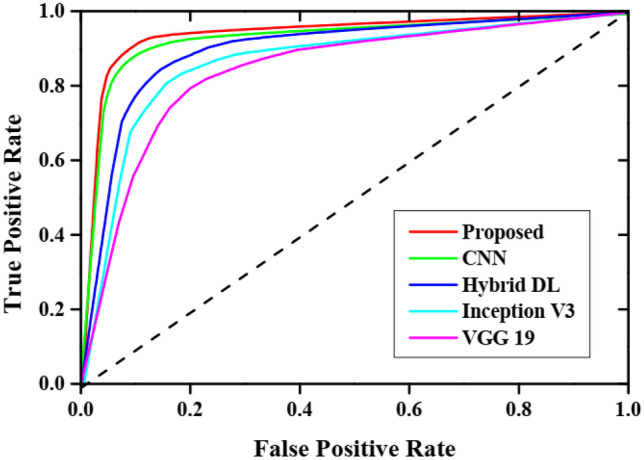
ROC curve
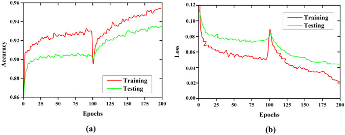
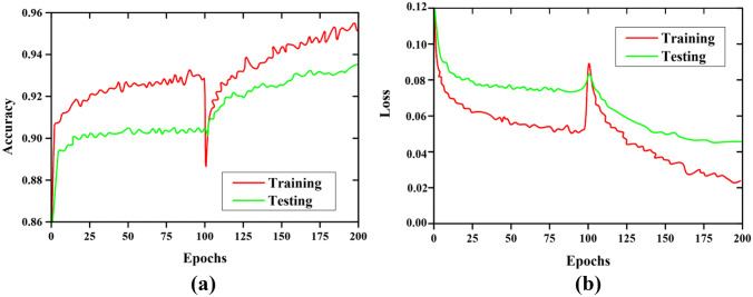
The training and testing accuracy and loss curve for MFCRNN-isPLI and VGG19 method is delineated in Figs. 6a, b and 7a, b. The presence of two curves represents the training and testing curves. Initially, the accuracy for testing is higher than training for a few epochs. The loss curve achieved for different epochs is presented in Figs. 6b and 7b. The lower loss rate depicts the improved generalization capability and faster convergence within a few epochs without getting struck.
Fig. 6.
Accuracy and loss curve validation of VGG19
Fig. 7.
Accuracy and loss curve evaluation for the proposed MFCRNN-isPLI method
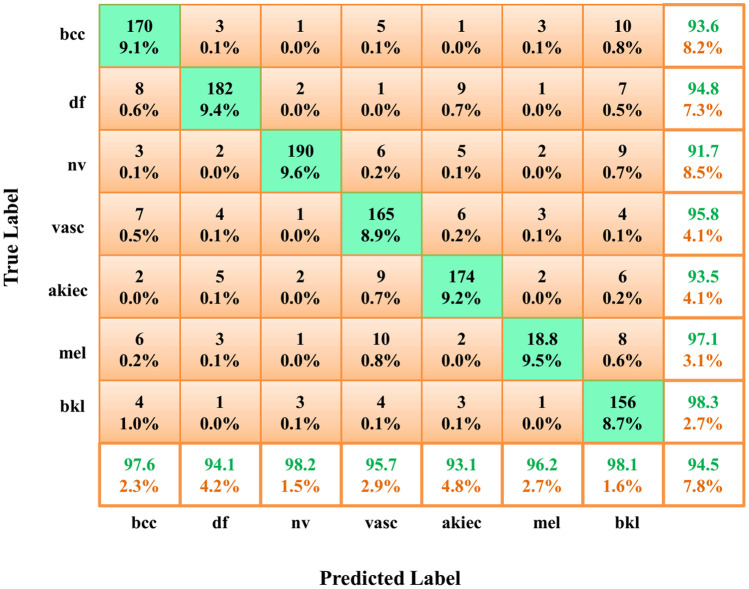
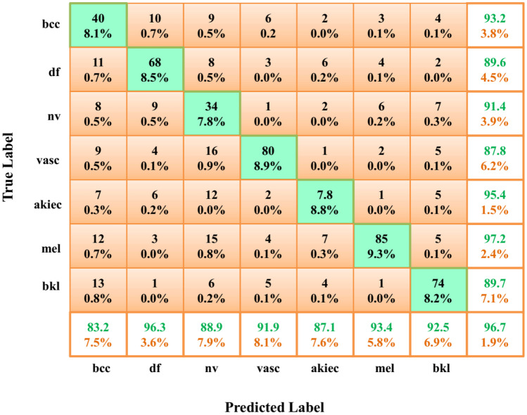
To understand the results more clearly, the confusion matrix helps. The confusion matrix incorporates more details about the accuracy and performance of the MFCRNN-isPLI method as it is a correlation between the predicted values and the true label of the classification method. The confusion matrix of the ISIC 2019 Skin Lesion images dataset and HAM10000 dataset is depicted in Figs. 8 and 9, respectively. The output of the classification is categorized as four. The misclassified positive image is called a false positive, and if it is predicted correctly, it is referred to as a true positive. If the healthy image is classified correctly as negative, it is called a true negative else it is called a false negative. The confusion matrix clearly explains the misclassification and accurate classification percentage values for the eight output classes of the ISIC 2019 skin lesion image dataset and eight classes of the HAM10000 dataset. The misclassification falls below 2% in all datasets. So the confusion matrix further confirms the diagnosing and classification accuracy of the model.
Fig. 8.
Confusion matrix of the ISIC 2019 Skin lesion image dataset
Fig. 9.
Confusion matrix of the HAM10000 dataset
Statistical Analysis Using Friedman–Nemenyi Test
The differences among the different skin cancer classification models are analyzed using the standard statistical test called Friedman–Nemenyi test. The analysis performance is based on accuracy while testing with the ISIC 2019 Skin Lesion images dataset and HAM10000 dataset. The analysis outputs are plotted in Fig. 10. Every dataset distinctly classified all the classifiers based on their ranks, and the average ranks are compared in the Friedman test. According to the null hypothesis, the classifiers which have similar values are not taken into consideration. The postdoc test of Nemenyi compared all the classifiers through critical distance (CD). The CD is computed in Eq. 36,
| 36 |
where q is the critical value obtained from the Nemenyi distribution table for a specific significance level (e.g., 0.05 for a 5% significance level) , k is the number of classifiers being compared, n is the number of samples or observations (e.g., number of instances in the dataset).
Fig. 10.
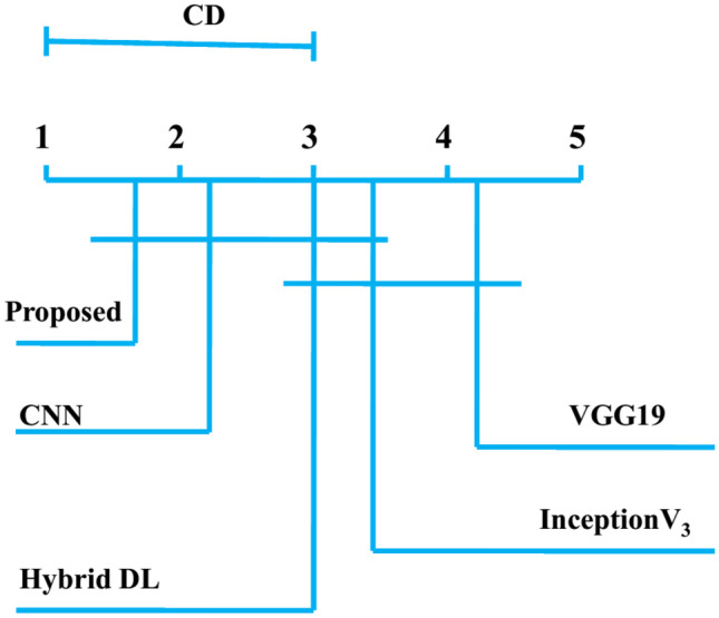
Friedman–Nemenyi test
If the average value of the two classifiers exceeds their critical distance, then there is a difference between the same classifiers. The existing CNN has also greater accuracy, but it is lesser than the MFCRNN-isPLI method. VGG19 attained less accuracy among all the methods.
Statistical Analysis
The statistical analysis of the proposed method is determined by using Statistical Package for Social Science (SPSS) on IBM PC. The data is evaluated independently by ANOVA. Tables 6 and 7 depict the statistical analysis of ISIC 2019 and HAM 10000 datasets. When compared with F ratio values, the combined dataset generates high dispersion result.
Table 6.
Statistical result analysis for ANOVA test for ISIC 2019 dataset
| DF | Sum of Sq | Mean Sq | F ratio | P value | |
|---|---|---|---|---|---|
| Model | 2 | 1.036 | 0.624 | 2.985 | 0.0636284 |
| Error | 197 | 36.642 | 0.196 | ||
| Total | 198 | 37.618 |
Table 7.
Statistical result analysis for ANOVA test for HAM 10000 dataset
| DF | Sum of Sq | Mean Sq | F ratio | P value | |
|---|---|---|---|---|---|
| Model | 2 | 2.927 | 1.428 | 2.393 | 0.100948 |
| Error | 75 | 40.728 | 0.587 | - | - |
| Total | 78 | 43.452 | - | - | - |
Discussion
Skin cancer affection is determined based on various issues, and a huge number of people are affected due to environmental conditions. The additional growth of abnormal cells in the skin leads to skin cancer. Based on their features and seriousness, it classifies the type. To categorize the type of skin cancer, various methods are discussed by the authors for accurate classification [16, 28, 31]. So it is significant to detect skin cancer at an early stage, and this helps to prevent the serious affection of cancer. To perform better classification, the deep learning method is more effective and it validates with multiple images. CNN, HDL, deep CNN, and VGG are some of the existing methods to detect and classify the type of skin cancer. But these methods were not detecting skin cancer accurately due to some of the limitations. To attain better performance, it requires huge training data sets as well as maximized consumption time. The multi-class classification is performed with high computational time as well as it does not satisfy real-world applications. So MFRCNN-iSPLI method is proposed to classify the type of skin cancer as well as the stage such as malignant or benign. The classification of the image is performed with faster RCNN. The datasets such as ISIC 2019 skin lesion image classification and HAM10000 are obtained to evaluate the efficiency of the proposed method with the existing method. The overfitting of the data features is prevented by the faster RCNN method by integrating with iSPLInception. The accuracy and the computational speed are enhanced which supports real-time skin cancer prediction.
Usually, when dealing with a class-imbalanced dataset in multi-class classification, enhancing stability for the method becomes a significant challenge. To address this, a two-CNN model is generated in parallel to analyze the performance of MFRCNN-iSPLI based on ResNet50 and VGG16 architectures. To enhance the training dataset, various augmentation techniques such as flipping, scaling, and traditional rotation methods are employed. This enlarged dataset is then used for training the model. For testing, both labeled and unlabeled data are used.
The classification of skin cancer is employed by the deep learning method. The proposed MFRCNN-iSPLI method is used to classify the type of skin cancer and also it reduces the overfitting issue. The datasets ISIC 2019 and HAM10000 are obtained to evaluate the performance. The proposed method is validated with various metrics and the comparison is performed with existing methods CNN, hybrid DL, Inception v3, and VGG19. The existing method requires more training time, the segmented images are not able to classify the type of skin cancer, as well as the presence of multiple images was not able to detect the skin cancer type accurately. This diminished the performance of the state-of-the-art methods. The increase in accuracy will improve the efficiency of the proposed method and obtain superior results.
After validating the accuracy of the proposed method attained 95.824% and the existing methods reduced the accuracy by 93.852%, 86.238%, 88.851%, and 87.825%, respectively. However, the proposed model does not perform feature extraction using different biomarkers such as pathological data, genomic profiles, and protein sequences. Another limitation of this model is that it is not evaluated using skin cancer images with low illumination and complex background retrieved from smartphones. So in the future, this method is extended to identify other disorders with large samples and we also plan to incorporate a lightweight security technique for efficient information sharing.
Conclusion
Over recent years, skin cancer incidences are growing rapidly. Thus, there is an urgent necessity to resolve this health challenge. Existing skin disease classification models poses various challenge in terms of accuracy, time taken, etc. Thus, an efficient method called MFCRNN-isPLI is presented in this paper. Instead of using the traditional selective search approach, the RPN is utilized by the FRCNN which reduces time overhead while selecting candidate regions, thus enhancing detection speed. For justifying this approach two skin disease datasets of ISIC 2019 Skin lesion image classification (includes eight classes and a normal class) and the HAM10000 dataset (includes seven different skin diseases) are taken. Accuracy, precision, recall, and F1-score values of the method are computed, and the outputs are compared with those of the four existing methods of CNN, hybrid DL, Inception v3, and VGG19. The output analysis of every measure confirmed the prediction and classification efficiency of the method with 95.82% accuracy, 96.85% precision, 96.52% recall, and 0.95% F1 score values. The Friedman–Nemenyi test is conducted to further analyze the performance which again confirms the proposed method’s accuracy. Thus, MFCRNN-isPLI is a promising approach for the classification and diagnosis of skin cancer. In the future, this technique expanded to varied diseases including more output classes which will increase the accuracy of the method.
Author Contribution
All authors agreed on the content of the study. JR, RRPBV, AS, and KS collected all the data for analysis. JR agreed on the methodology. JR, RRPBV, AS, and KS completed the analysis based on agreed steps. Results and conclusions are discussed and written together. The author read and approved the final manuscript.
Availability of Data and Material
The data that support the findings of this study are available from the corresponding author upon reasonable request.
Code Availability
Not applicable.
Declarations
Ethics Approval
This article does not contain any studies with human participants.
Consent to Participate
Not applicable.
Consent for Publication
Not applicable.
Informed Consent
Informed consent was obtained from all individual participants included in the study.
Human and Animal Rights
This article does not contain any studies with human or animal subjects performed by any of the authors.
Conflict of interest
The authors declare no competing interests.
Footnotes
Publisher's Note
Springer Nature remains neutral with regard to jurisdictional claims in published maps and institutional affiliations.
References
- 1.Bhatt H, Shah V, Shah K, Shah R, Shah M: State-of-the-art machine learning techniques for melanoma skin cancer detection and classification: a comprehensive review. Intelligent Medicine 2022
- 2.Zhang N, Cai YX, Wang YY, Tian YT, Wang XL, Badami B. Skin cancer diagnosis based on optimized convolutional neural network. Artificial intelligence in medicine. 2020;102:101756. doi: 10.1016/j.artmed.2019.101756. [DOI] [PubMed] [Google Scholar]
- 3.Pacheco AG, Krohling RA. The impact of patient clinical information on automated skin cancer detection. Computers in biology and medicine. 2020;116:103545. doi: 10.1016/j.compbiomed.2019.103545. [DOI] [PubMed] [Google Scholar]
- 4.Tan TY, Zhang L, Lim CP. Intelligent skin cancer diagnosis using improved particle swarm optimization and deep learning models. Applied Soft Computing. 2019;84:105725. doi: 10.1016/j.asoc.2019.105725. [DOI] [Google Scholar]
- 5.Murugan A, Nair SAH, Kumar KP. Detection of skin cancer using SVM, random forest and kNN classifiers. Journal of medical systems. 2019;43(8):1–9. doi: 10.1007/s10916-019-1400-8. [DOI] [PubMed] [Google Scholar]
- 6.Jones OT, Matin RN, van der Schaar M, Bhayankaram KP, Ranmuthu CKI, Islam MS, Behiyat D, Boscott R, Calanzani N, Emery J, Williams HC. Artificial intelligence and machine learning algorithms for early detection of skin cancer in community and primary care settings: a systematic review. The Lancet Digital Health. 2022;4(6):e466–e476. doi: 10.1016/S2589-7500(22)00023-1. [DOI] [PubMed] [Google Scholar]
- 7.Hekler A, Utikal JS, Enk AH, Hauschild A, Weichenthal M, Maron RC, Berking C, Haferkamp S, Klode J, Schadendorf D, Schilling B. Superior skin cancer classification by the combination of human and artificial intelligence. European Journal of Cancer. 2019;120:114–121. doi: 10.1016/j.ejca.2019.07.019. [DOI] [PubMed] [Google Scholar]
- 8.Sankareswaran SP, Krishnan M: Unsupervised end-to-end brain tumor magnetic resonance image registration using RBCNN: rigid transformation, B-spline transformation and convolutional neural network. Current Medical Imaging 18(4):1, 2022. 10.2174/1573405617666210806125526 [DOI] [PubMed]
- 9.Senthil Pandi S, Senthilselvi A, Gitanjali J, ArivuSelvan K, Gopal J, Vellingiri J: Rice plant disease classification using dilated convolutional neural network with global average pooling. Ecological Modelling 474:110166, 2022 ISSN 0304-3800. 10.1016/j.ecolmodel.2022.110166
- 10.E., D., S., S.P., R., P. et al. Artificial humming bird optimization–based hybrid CNN-RNN for accurate exudate classification from fundus images. J Digit Imaging 36:59–72, 2023. 10.1007/s10278-022-00707-7 [DOI] [PMC free article] [PubMed]
- 11.Senthil Pandi S, Senthilselvi A, Maragatharajan M, Manju I: An optimal self adaptive deep neural network and spine-kernelled chirplet transform for image registration. Concurrency and Computation: Practice and Experience 34(27):e7297, 2022. 10.1002/cpe.7297
- 12.Kalpana B, Reshmy AK, Senthil Pandi S, Dhanasekaran S: OESV-KRF: optimal ensemble support vector kernel random forest based early detection and classification of skin diseases. Biomedical Signal Processing and Control, 85:104779 2023 ISSN 1746-8094. 10.1016/j.bspc.2023.104779
- 13.Chaturvedi SS, Tembhurne JV, Diwan T. A multi-class skin Cancer classification using deep convolutional neural networks. Multimedia Tools and Applications. 2020;79(39):28477–28498. doi: 10.1007/s11042-020-09388-2. [DOI] [Google Scholar]
- 14.Saba T, Khan MA, Rehman A, Marie-Sainte SL. Region extraction and classification of skin cancer: A heterogeneous framework of deep CNN features fusion and reduction. Journal of medical systems. 2019;43(9):1–19. doi: 10.1007/s10916-019-1413-3. [DOI] [PubMed] [Google Scholar]
- 15.Senan EM, Jadhav ME. Analysis of dermoscopy images by using ABCD rule for early detection of skin cancer. Global Transitions Proceedings. 2021;2(1):1–7. doi: 10.1016/j.gltp.2021.01.001. [DOI] [Google Scholar]
- 16.Sheha MA, Mabrouk MS, Sharawy A. Automatic detection of melanoma skin cancer using texture analysis. International Journal of Computer Applications. 2012;42(20):22–26. doi: 10.5120/5817-8129. [DOI] [Google Scholar]
- 17.Imran A, Nasir A, Bilal M, Sun G, Alzahrani A, Almuhaimeed A: Skin Cancer detection using Combined Decision of Deep Learners. IEEE Access 2022
- 18.Maniraj SP, Maran PS: A hybrid deep learning approach for skin cancer diagnosis using subband fusion of 3D wavelets. The Journal of Supercomputing 1–16,2022
- 19.Shorfuzzaman M. An explainable stacked ensemble of deep learning models for improved melanoma skin cancer detection. Multimedia Systems. 2022;28(4):1309–1323. doi: 10.1007/s00530-021-00787-5. [DOI] [Google Scholar]
- 20.Narunsky-Haziza L, Sepich-Poore GD, Livyatan I, Asraf O, Martino C, Nejman D, Gavert N, Stajich JE, Amit G, González A, Wandro S. Pan-cancer analyses reveal cancer-type-specific fungal ecologies and bacteriome interactions. Cell. 2022;185(20):3789–3806. doi: 10.1016/j.cell.2022.09.005. [DOI] [PMC free article] [PubMed] [Google Scholar]
- 21.Kausar N, Hameed A, Sattar M, Ashraf R, Imran AS, Abidin MZU, Ali A. Multiclass Skin Cancer Classification Using Ensemble of Fine-Tuned Deep Learning Models. Applied Sciences. 2021;11(22):10593. doi: 10.3390/app112210593. [DOI] [Google Scholar]
- 22.Sripada NK, Mohammed Ismail B: A Multi-Class Skin Cancer Classification Through Deep Learning. In Evolutionary Computing and Mobile Sustainable Networks (pp. 527–539). Springer, Singapore. 2022
- 23.Ali K, Shaikh ZA, Khan AA, Laghari AA: Multiclass skin cancer classification using EfficientNets–a first step towards preventing skin cancer. Neuroscience Informatics 100034,2021
- 24.Zeng L, Sun B, Zhu D. Underwater target detection based on Faster R-CNN and adversarial occlusion network. Engineering Applications of Artificial Intelligence. 2021;100:104190. doi: 10.1016/j.engappai.2021.104190. [DOI] [Google Scholar]
- 25.Bai T, Yang J, Xu G, Yao D. An optimized railway fastener detection method based on modified Faster R-CNN. Measurement. 2021;182:109742. doi: 10.1016/j.measurement.2021.109742. [DOI] [Google Scholar]
- 26.Ezugwu AE, Agushaka JO, Abualigah L, Mirjalili S, Gandomi AH. Prairie dog optimization algorithm. Neural Computing and Applications. 2022;34(22):20017–20065. doi: 10.1007/s00521-022-07530-9. [DOI] [PMC free article] [PubMed] [Google Scholar]
- 27.Ronald M, Poulose A, Han DS. iSPLInception: an inception-ResNet deep learning architecture for human activity recognition. IEEE Access. 2021;9:68985–69001. doi: 10.1109/ACCESS.2021.3078184. [DOI] [Google Scholar]
- 28.Ali MS, Miah MS, Haque J, Rahman MM, Islam MK. An enhanced technique of skin cancer classification using deep convolutional neural network with transfer learning models. Machine Learning with Applications. 2021;5:100036. doi: 10.1016/j.mlwa.2021.100036. [DOI] [Google Scholar]
- 29.Larxel: (2020, May 28). Skin lesion images for melanoma classification. Kaggle. Retrieved November 21, 2022, from https://www.kaggle.com/datasets/andrewmvd/isic-2019
- 30.Tschandl P: (2021, January 29). The HAM10000 dataset is a large collection of multi-source dermatoscopic images of common pigmented skin lesions. Harvard Dataverse. Retrieved November 21, 2022, from https://dataverse.harvard.edu/dataset.xhtml?persistentId=doi%3A10.7910%2FDVN%2FDBW86T [DOI] [PMC free article] [PubMed]
- 31.Srinivasu PN, SivaSai JG, Ijaz MF, Bhoi AK, Kim W, Kang JJ. Classification of skin disease using deep learning neural networks with MobileNet V2 and LSTM. Sensors. 2021;21(8):2852. doi: 10.3390/s21082852. [DOI] [PMC free article] [PubMed] [Google Scholar]
Associated Data
This section collects any data citations, data availability statements, or supplementary materials included in this article.
Data Availability Statement
The data that support the findings of this study are available from the corresponding author upon reasonable request.
Not applicable.


