Value of information for a leader–follower partially observed Markov game

Abstract

We consider a leader–follower partially observed Markov game (POMG) and analyze how the value of the leader’s criterion changes due to changes in the leader’s quality of observation of the follower. We give conditions that insure improved observation quality will improve the leader’s value function, assuming that changes in the observation quality do not cause the follower to change its policy. We show that discontinuities in the value of the leader’s criterion, as a function of observation quality, can occur when the change of observation quality is significant enough for the follower to change its policy. We present conditions that determine when a discontinuity may occur and conditions that guarantee a discontinuity will not degrade the leader’s performance. We show that when the leader and the follower are collaborative and the follower completely observes the leader’s initial state, discontinuities in the leader’s value function will not occur. However, examples show that improving observation quality does not necessarily improve the leader’s criterion value, whether or not the POMG is a collaborative game.

Appendices

Appendix 1: Proofs

Proof of Theorem 1

Proof of Theorem 1 is given in White and Harrington (1980).$\square$

Proof of Corollary 1

Proof of (a) follows from the fact that an optimal policy has a concave value function and can be found in White and Harrington (1980) and Zhang (2010). Proof of (b) follows from the facts that for any stochastic matrix $Q'$, there are stochastic matrices R and $R''$ such that $Q'R = Q$ and $Q''R'' = Q'$. $\square$

Proof of Proposition 1

Proof follows the proof of Proposition 2 in Chang et al. (2014). $\square$

Proof of Proposition 2

Proof follows from Lemma 1 in Ortiz et al. (2013) and Proposition 2 in Chang et al. (2014). $\square$

Proof of Corollary 2

(1) follows directly from Theorem 1 and Proposition 1. It is sufficient to show that $v^L(\pi ^L, \pi ^F, Q)(d^L(t,\tau ), y^L(t))$ is concave in $y^L(t)$ for (2) to hold. It follows from Proposition 2 that

$$\begin{aligned}&v^L(\pi ^L, \pi ^F, Q)(d^L(t,\tau ), y^L(t)) \\&\quad = \max _{\rho ^L} \sum _{d^F(t,\tau )}P(d^F(t,\tau )|d^L(t)) g^L(d(t,\tau ), \rho ^L, \pi ^*(\rho ^L, Q),Q), \end{aligned}$$

which is concave in $y^L(t)$. $\square$

Proof of Proposition 3

For any scalar valued function v dependent on $(d(t,\tau ))$, define

$$\begin{aligned}&[Hv](d(t,\tau )) = R^L(d(t,\tau ),\pi ^L, \pi ^F) \\&\quad +\beta \sum _{\varsigma (t+1)} P(\varsigma (t+1)|d(t,\tau ), \pi ^L, \pi ^F,Q) \times v(\{\varsigma (t+1), d(t,\tau -1)\}). \end{aligned}$$

Define $H'$ identically to H but replace Q by $Q'$, where we note:

$$\begin{aligned}&P(\varsigma (t+1)|d(t,\tau ),\pi ^L, \pi ^F,Q) \\&\quad = \sum _{a(t)}P(a(t)|d(t,\tau ))P(z^L(t+1)|s^F(t+1))P(z^F(t+1), s(t+1)|s(t),a(t)). \end{aligned}$$

Let g and $g'$ be the fixed points of H and $H'$, respectively [Existence and uniqueness of these fixed points are assured by Theorem 6.2.3 in Puterman (1994)]. Then,

$$\begin{aligned}&g(d(t,\tau )) \!-\! g'(d(t,\tau ))\!=\! [Hg](d(t,\tau )) - [H'g'](d(t,\tau )) \!-\! [Hg'](d(t,\tau )) \!+ \)\\&\quad =\beta \sum _{a(t)}P(a(t)|d(t,\tau )) \times X, \end{aligned}$$

where

$$\begin{aligned} X&=\sum _{z(t+1)}\sum _{s(t+1)}P(z(t+1),s(t+1)|s(t),a(t))\\&\quad \times \{g(\{\varsigma (t+1), d(t,\tau -1)\})-g'(\{\varsigma (t+1), d(t,\tau -1)\})\}\\&\quad +\sum _{z(t+1)}\sum _{s(t+1)}[P(z^L(t+1)|s^F(t+1))-P'(z^L(t+1)|s^F(t+1))]P(z^F(t+1),\\&\qquad s(t+1)|s(t), a(t))\times g'(\{\varsigma (t+1), d(t,\tau -1)\}) \end{aligned}$$

Note, $||g'|| \le \frac{M}{1-\beta }$, where $M = \max _{s}\max _a r^L(s,a)$. Then, it is straightforward to show that

$$\begin{aligned} ||g-g'|| \le \beta ||g-g'|| + \beta ||Q-Q'||\frac{M}{1-\beta } \end{aligned}$$

and hence,

$$\begin{aligned} ||g-g'|| \le \frac{\beta M}{(1-\beta )^2}||Q-Q'||. \end{aligned}$$

$\square$

Proof of Proposition 4

If Q is such that

$$\begin{aligned} v^F(\pi ^L, \pi ^F, Q)(d^F(0)) - v^F(\pi ^L, \rho ^F, Q)(d^F(0)) \ge 0 \end{aligned}$$

for all $\rho ^F \ne \pi ^F, \rho ^F, \pi ^F \in \Pi ^F$ and given $d^F(0)$, then $Q \in K(\pi ^L, \pi ^F)$. Note

$$\begin{aligned}&v^F(\pi ^L, \pi ^F, Q)(d^F(0)) - v^F(\pi ^L, \rho ^F, Q)(d^F(0))\\&\quad = v^F(\pi ^L, \pi ^F, Q)(d^F(0)) - v^F(\pi ^L, \pi ^F, Q')(d^F(0)) + v^F(\pi ^L, \rho ^F, Q')(d^F(0)) \\&\qquad - v^F(\pi ^L, \rho ^F, Q)(d^F(0)) + v^F(\pi ^L, \pi ^F, Q')(d^F(0)) - v^F(\pi ^L, \rho ^F, Q')(d^F(0)) \\&\quad \ge -\frac{2\beta M}{(1-\beta )^2} ||Q-Q'||+b, \end{aligned}$$

where the inequality follows from Proposition 3 and definitions of b and M. The result follows from the fact that $b -\frac{2\beta M}{(1-\beta )^2} ||Q-Q'|| \ge 0$ if and only if $||Q-Q'||\le \frac{b(1-\beta )^2}{2\beta M}$. $\square$

Proof of Lemma 1

The proof follows from Proposition 4.7.3 (Puterman, p. 106) and a standard limit procedure. $\square$

Proof of Proposition 5

Lemma 1 guarantees that $g^L(d^L(t,\tau ), Q^*, \pi ^L, \pi ')$ for $\pi ' \!\in \! \{\pi ^F, \rho ^F\}$ is isotone in $d(t,\tau )$. It follows from Lemma 4.7.2 (Puterman, p. 106) that

$$\begin{aligned}&\sum _{\varsigma (t+1)} P(\varsigma (t+1)|d(t,\tau ), Q^*, \pi ^L, \rho ^F) \times g^L(d(t,\tau )| Q^*, \pi ^L, \pi ^F) \\&\quad \ge \sum _{\varsigma (t+1)} P(\varsigma (t+1)|d(t,\tau ), Q^*, \pi ^L, \pi ^F) \times g^L(d(t,\tau )| Q^*, \pi ^L, \pi ^F). \end{aligned}$$

Thus,,

$$\begin{aligned}&g^L(d(t,\tau ), Q^*, \pi ^L, \pi ^F) \nonumber \\&\quad \le R^L(d(t,\tau ), \pi ^L, \rho ^F) +\beta \sum _{\varsigma (t+1)} P (\varsigma (t+1)|Q^*, \pi ^L, \rho ^F) \times g^L(d(t,\tau ), Q^*, \pi ^L, \pi ^F). \end{aligned}$$

(6)

Let

$$\begin{aligned}&[Hv](d(t,\tau )) \\&\quad = R^L(d(t,\tau ), \pi ^L, \rho ^F) + \beta \sum _{\varsigma (t+1)}P(\varsigma (t+1)|d(t,\tau ), Q^*, \pi ^L, \rho ^F)\\&\quad \times v(\{\varsigma (t+1), d(t,\tau -1)\}). \end{aligned}$$

Define the sequence $\{v^n\}$ as $v^{n+1} = Hv^n$, where $v^0(d(t,\tau )) = g^L(d(t,\tau ), Q^*, \pi ^L, \pi ^F)$. We remark that $\lim _{n \rightarrow \infty } ||v^n - v^*|| = 0$, where $v^*(d(t,\tau )) = g^L(d(t,\tau ), Q^*, \pi ^L, \rho ^F).$ It is straightforward to show that $v \le v'$ implies $Hv \le Hv'$. Eq. (6) has shown $v^0 \le v^1$. Lemma 1 guarantees that $v^n$ is isotone in $d(t,\tau )$ for $n \ge 1$. Hence, by induction, $v^n \le v^{n+1}$ and therefore $v^n \le v^*$ for all n. Thus, $g^L(d(t,\tau ), Q^*, \pi ^L, \pi ^F) \le g^L(d(t,\tau ), Q^*, \pi ^L, \rho ^F)$ for all $d(t,\tau )$ and hence $v^L(\pi ^L, \pi ^F, Q^*)(d^L(0)) \le v^L(\pi ^L, \rho ^F, Q^*)(d^L(0))$. $\square$

Proof of Proposition 6

Assumption (1) implies that $v^F(\pi ^L, \pi ', Q^*)(d^F(0)) = g^F(d(0,\tau ), Q^*, \pi ^L, \pi ')$ for $\pi ' \in \{\pi ^F, \rho ^F \}.$ Assumption (2) implies $v^F(\pi ^L, \pi ^F, Q^*)(d^F(0)) = v^F(\pi ^L, \rho ^F, Q^*)(d^F(0))$. Hence, $g^F(d(0,\tau ), \pi ^L, \pi ^F)=g^F(d(0,\tau ), \pi ^L, \rho ^F)$. Assumption (3) implies $g^L=g^F$. $\square$

Appendix 2: Parameters for the examples

The parameters in Example 1 are:

• transition probabilities:

  $$\begin{aligned} P^L(1)= & {} \begin{bmatrix} 0.6229&0.3771\\ 0.7506&0.2494 \end{bmatrix}, P^L(2)=\begin{bmatrix} 0.7531&0.2469\\ 0.1761&0.8239 \end{bmatrix}\\ P^F(1)= & {} \begin{bmatrix} 0.2232&0.7768\\ 0.5131&0.4869 \end{bmatrix}, P^F(2)=\begin{bmatrix} 0.9449&0.0551\\ 0.2663&0.7337 \end{bmatrix} \end{aligned}$$

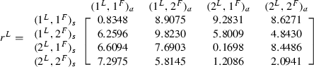
• reward structure $r^k(s^L,s^F,a^L,a^F), k \in \{L,F\}$:

  

  • (1) example(a):

    

  • (2) example(b):

    

  • (3) example(c):

    

  • (4) example(d):

    

  • (5) example(e):

    

  • (6) example(f):

    

The parameters in Example 2 are:

• transition probabilities: $P(s(t+1),z^F(t+1)|s(t),\pi ^L, \rho ^F)=$

  

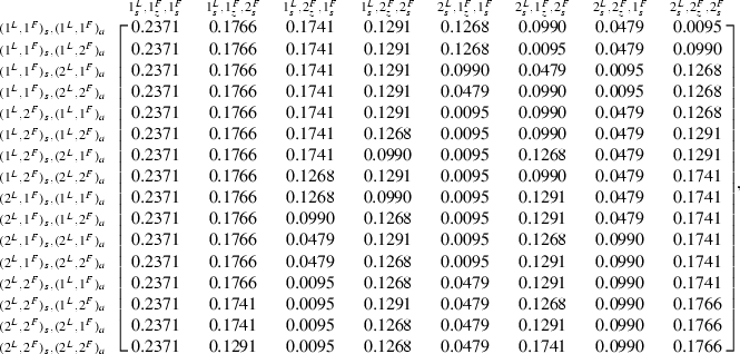
  $P(s(t+1),z^F(t+1)|s(t),\pi ^L, \pi ^F)=$

  
  $$\begin{aligned} Q^{L*} \in K(\pi ^L, \pi ^F) \cap K(\pi ^L, \rho ^F), Q^{L*}=\begin{bmatrix} 0.6&0.4\\ 0.4&0.6 \end{bmatrix} \end{aligned}$$

• reward structure: $R^F(d^F(t,\tau ),\pi ^L,\rho ^F)=[2.0944, -10, 9.1798, -10, 9.1768, -10, 9.1858,$ $-10,-10, 9.3521, -10, 9.3522, -10, 9.3620, -10, 2.8030]$ $R^F(d^F(t,\tau ),\pi ^L,\pi ^F)=[3.3540, 10, -9.3656, 10, -9.3656, 10, -9.3656, 10,$ $10, -9.3656, 10, -9.3656, 10, -9.3656, 10, -9.3656]$ $R^F(d^F(t,\tau ),\rho ^L,\rho ^{F'}) = -\infty , \forall \rho ^{F'} \in \Pi ^F$ $R^L(d^F(t,\tau ),\pi ^L,\rho ^F)=[2.9118,2.8947, 2.8725, 2.8715, 2.7401, 2.7174, 2.4442, 2.4008,$ 1.8971, 1.6406, 1.4561, 0.8355, 0.4728, 0.4257, 0.3810, 0.2926] $R^L(d^F(t,\tau ),\pi ^L,\pi ^F)=[2.0224, 1.9607, 1.9596, 1.9568, 1.9523, 1.9479, 1.7010, 1.6948,$ 1.2183, 0.9849, 0.8006, 0.4137, 0.3452, 0.2608, 0.2545, 0.0806]

The parameters in Example 3 are:

• (1) example(a):

  • transition probabilities:

    $$\begin{aligned} P^L(1)= & {} \begin{bmatrix} 0.3202&0.6798\\ 0.3044&0.6956 \end{bmatrix}, P^L(2)=\begin{bmatrix} 0.7624&0.2376\\ 0.3790&0.6210 \end{bmatrix}\\ P^F(1)= & {} \begin{bmatrix} 0.2593&0.7407\\ 0.6356&0.3644 \end{bmatrix}, P^F(2)=\begin{bmatrix} 0.5221&0.4779\\ 0.0994&0.9006 \end{bmatrix} \end{aligned}$$

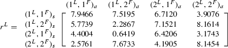
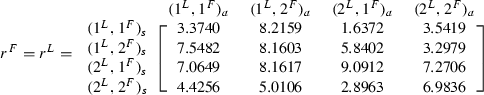
  • reward structure $r^k(s^L,s^F,a^L,a^F), k \in \{L,F\}$:

    

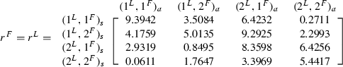
• (2) example(b):

  • transition probabilities:

    $$\begin{aligned} P^L(1)= & {} \begin{bmatrix} 0.3277&0.6723\\ 0.9623&0.0377 \end{bmatrix}, P^L(2)=\begin{bmatrix} 0.4723&0.5277\\ 0.4469&0.5531 \end{bmatrix}\\ P^F(1)= & {} \begin{bmatrix} 0.8815&0.1185\\ 0.6147&0.3853 \end{bmatrix}, P^F(2)=\begin{bmatrix} 0.0641&0.9359\\ 0.2062&0.7938 \end{bmatrix} \end{aligned}$$

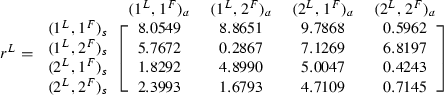
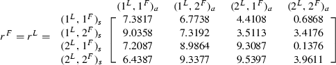
  • reward structure $r^k(s^L,s^F,a^L,a^F), k \in \{L,F\}$:

    

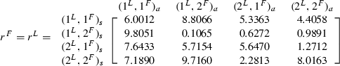
• (3) example(c):

  • transition probabilities:

    $$\begin{aligned} P^L(1)= & {} \begin{bmatrix} 0.7657&0.2343\\ 0.9270&0.0730 \end{bmatrix}, P^L(2)=\begin{bmatrix} 0.5570&0.4430\\ 0.8113&0.1887 \end{bmatrix}\\ P^F(1)= & {} \begin{bmatrix} 0.3594&0.6406\\ 0.0007&0.9993 \end{bmatrix}, P^F(2)=\begin{bmatrix} 0.4647&0.5353\\ 0.7964&0.2036 \end{bmatrix} \end{aligned}$$

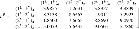
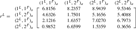
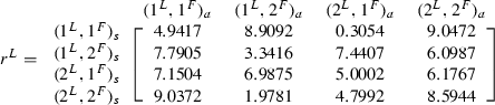
  • reward structure $r^k(s^L,s^F,a^L,a^F), k \in \{L,F\}$:

    

• (4) example(d):

  • transition probabilities:

    $$\begin{aligned} P^L(1)= & {} \begin{bmatrix} 0.5983&0.4017\\ 0.6592&0.3408 \end{bmatrix}, P^L(2)=\begin{bmatrix} 0.8785&0.1215\\ 0.3068&0.6932 \end{bmatrix}\\ P^F(1)= & {} \begin{bmatrix} 0.7036&0.2964\\ 0.5885&0.4115 \end{bmatrix}, P^F(2)=\begin{bmatrix} 0.0593&0.9407\\ 0.3593&0.6407 \end{bmatrix} \end{aligned}$$

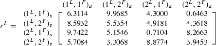
  • reward structure $r^k(s^L,s^F,a^L,a^F), k \in \{L,F\}$:

References

Bassan, B., Gossner, O., Scarsini, M., & Zamir, S. (2003). Positive value of information in games. Internal Journal of Game Theory, 32, 17–31.
Bertsekas, D. P. (1976). Dynamic programming and stochastic control. New York: Academic Press.
Bernstein, D. S., Givan, R., Immerman, N., & Zilberstein, S. (2002). The complexity of decentralized control of Markov decision processes. Mathematics of Operations Research, 27(4), 819–840.
Bier, V. M., Oliveros, S., & Samuelson, L. (2007). Choosing what to protect: Strategic defensive allocation against an unknown attacker. Journal of Public Economic Theory, 9(4), 563–587.
Cassandra, A. R., Kaelbling, L. P., & Littman, M. L. (1994). Acting optimally in partially observable stochastic domains. In Proceedings twelfth national conference on artificial intelligence (AAAI-94) (pp. 1023–1028). WA: Seattle.
Cassandra, A. R., Littman, M. L., & Zhang, N. L. (1997). Incremental pruning: A simple, fast, exact method for partially observable Markov decision processes. In Proceedings thirteenth annual conference on uncertainty in artificial intelligence (UAI-97) (pp. 54–61). San Francisco, CA: Morgan Kaufmann.
Chang, Y. L., Erera, A.L., & White, C. C. (2014). A leader–follower partially observed multiobjective Markov game, submitted for publication.
Chu, W. H. J., & Lee, C. C. (2006). Strategic information sharing in a supply chain. European Journal of Operational Reserch, 174, 1567–1579.
Ezell, B. C., Bennett, S. P., von Winterfeldt, D., Sokolowski, J., & Collins, A. J. (2010). Probabilistic risk analysis and terrorism risk. Risk Analysis, 30(4), 575–589.
Hansen, E. A., Bernstein, D. S., & Zilberstein, S. (2004). Dynamic programming for partially observable stochastic games. In Proceedings of the nineteenth national conference on artificial intelligence (pp. 709–715). San Jose: California.
Kamien, M. I., Tauman, Y., & Zamir, S. (1990). On the value of information in a strategic conflict. Games and Economic Behavior, 2, 129–153.
Kumar, A., & Zilberstein, S. (2009). Dynamic programming approximations for partially observable stochastic games. In Proceedings of the twenty-second international FLAIRS conference (pp. 547–552). Florida: Sanibel Island.
Lehrer, E., & Rosenberg, D. (2006). What restrictions do Bayesian games impose on the value of information? Journal of Mathematical Economics, 42, 343–357.
Lehrer, E., & Rosenberg, D. (2010). A note on the evaluation of information in zero-sum repeated games. Journal of Mathematical Economics, 46, 393–399.
Leng, M. M., & Parlar, M. (2009). Allocation of cost savings in a three-level supply chain with demand information sharing: A cooperate-game approach. Operations Research, 57(1), 200–213.
Li, L. (2002). Information sharing in a supply chain with horizontal competition. Management Science, 48(9), 1196–1212.
Lin, A. Z.-Z., Bean, J., & White, C. C. (1998). Genetic algorithm heuristics for finite horizon partially observed Markov decision problems, Technical report, University of Michigan, Ann Arbor.
Lin, A. Z.-Z., Bean, J., & White, C. C. (2004). A hybrid genetic/optimization algorithm for finite horizon partially observed Markov decision processes. Journal on Computing, 16(1), 27–38.
Littman, M. L. (1994). The Witness algorithm: solving partially observable Markov decision processes, Brown University, Department of Computer Science, Technical report, CS-94-40.
Lovejoy, W. S. (1991). A survey of algorithmic methods for partially observed Markov decision process. Annals of Operations Research, 28(1), 47–65.
Meuleau, N., Peshkin, L., Kim, K., & Kaelbling, L. P. (1999). Learning finite-state controllers for partially observable environments. In Proceedings of the fifteenth conference on uncertainty in artificial intelligence (pp. 427–436). Morgan Kaufmann Publishers.
Meyer, B. D., Lehrer, E., & Rosenberg, D. (2010). Evaluating information in zero-sum games with incomplete information on both sides. Mathematics of Operations Research, 35(4), 851–863.
Monahan, G. E. (1982). A survey of partially observable Markov decision processes: Theory, models, and algorithms. Management Science, 28, 1–16.
Ortiz, O. L., Erera, A. L., & White, C. C. (2013). State observation accuracy and finite-memory policy performance. Operations Research Letters, 41, 477–481.
Platzman, L. K. (1977). Finite memory estimation and control of finite probabilistic systems, PhD thesis, Cambridge, MA: Massachusetts Institute of Technology.
Platzman, L. K. (1980). Optimal infinite-horizon undiscounted control of finite probabilistic systems. SIAM Journal on Control and Optimization, 18, 362–380.
Poupart, P., & Boutilier, C. (2004). Bounded finite state controllers, Advances in Neural Information Processing Systems, 16. Cambridge, MA: MIT Press.
Puterman, M. L. (1994). Markov decision processes: Discrete dynamic programming. New York: Wiley.
Rabinovich, Z., Goldman, C. V., & Rosenschein, J. S. (2003). The complexity of multiagent systems: The price of silence. Proceedings of the second international joint conference on autonomous agents and multi-agent systems (AAMAS) (pp. 1102–1103). Australia, Melbourne.
Shapley, L. S. (1953). Stochastic games, Proceedings of the national academy of sciences of the USA, 39, 1095–1100.
Smallwood, R. D., & Sondik, E. J. (1973). The optimal control of partially observable Markov decision processes over a finite horizon. Operations Research, 21, 1071–1088.
Sondik, E. J. (1978). The optimal control of partially observable Markov processes over the infinite horizon: Discounted costs. Operations Research, 26, 282–304.
Wakker, P. (1988). Nonexpected utility as aversion of information. Journal of Behavioral Decision Making, 1, 169–175.
White, C. C., & Harrington, D. P. (1980). Application of Jensen’s inequality to adaptive suboptimal design. Journal of Optimization Theory and Application, 32, 89–99.
White, C. C., & Scherer, W. T. (1989). Solution procedures for partially observed Markov decision processes. Operations Research, 37, 791–797.
White, C. C. (1991). A survey of solution techniques for the partially observed Markov decision process. Annals of Operations Research, 32, 215–230.
White, C. C., & Scherer, W. T. (1994). Finite-memory suboptimal design for partially observed Markov decision processes. Operations Research, 42, 439–455.
Zhang, H. (2010). Partially observable Markov decision processes: A geometric technique and analysis. Operations Research, 58, 214–228.
Zhuang, J., & Bier, V. M. (2010). Reasons for secrecy and deception in homeland-security resource allocation. Risk Analysis, 30(12), 1737–1743.
Zhuang, J., Bier, V. M., & Alagoz, O. (2010). Modeling secrecy and deception in a multiple-period attacker-defender signaling game. European Journal of Operational Research, 203, 409–418.
Acknowledgments
This material is based upon work supported by the US Department of Homeland Security under Grant Award Number 2010-ST-061-FD0001 through a grant awarded by the National Center for Food Protection and Defense at the University of Minnesota. The views and conclusions contained in this document are those of the authors and should not be interpreted as necessarily representing the official policies, either expressed or implied, of the US Department of Homeland Security or the National Center for Food Protection and Defense.
Author information
Authors and Affiliations
Corresponding author