Handling uncertainty in SBSE: a possibilistic evolutionary approach for code smells detection

Abstract

Code smells, also known as anti-patterns, are poor design or implementation choices that hinder program comprehensibility and maintainability. While several code smell detection methods have been proposed, Mantyla et al. identified the uncertainty issue as one of the major individual human factors that may affect developer’s decisions about the smelliness of software classes: they may indeed have different opinions mainly due to their different knowledge and expertise. Unfortunately, almost all the existing approaches assume data perfection and neglect the uncertainty when identifying the labels of the software classes. Ignoring or rejecting any uncertainty form could lead to a considerable loss of information, which could significantly deteriorate the effectiveness of the detection and identification processes. Inspired by our previous works and motivated by the interesting performance of the PDT (Possibilistic Decision Tree) in classifying uncertain data, we propose ADIPE (Anti-pattern Detection and Identification using Possibilistic decision tree Evolution), as a new tool that evolves and optimizes a set of detectors (PDTs) that could effectively deal with software class labels uncertainty using some concepts from the Possibility theory. ADIPE uses a PBE (Possibilistic Base of Examples: a dataset with possibilistic labels) that it is built using a set of opinion-based classifiers (i.e., a set of probabilistic classifiers) with the aim to simulate human developers’ uncertainty. A set of advisors and probabilistic classifiers are employed in order to mimic the subjectivity and the doubtfulness of software engineers. A detailed experimental study is conducted to show the merits and outperformance of ADIPE in dealing with uncertainty in code smells detection and identification with respect to four relevant state-of-the-art methods, including the baseline PDT. The experimental study was performed in uncertain and certain environments based on two suitable metrics: PF-measure_dist (Possibilistic F-measure_Distance) and IAC (Information Affinity Criterion); which corresponds to the F-measure and Accuracy (PCC) for the certain case. The obtained results for the uncertain environment reveal that for the detection process, the PF-measure_dist of ADIPE ranges within [0.9047 and 0.9285], and its IAC lies within [0.9288 and 0.9557]; while for the identification process, the PF-measure_dist of ADIPE is in [0.8545, 0.9228], and its IAC lies within [0.8751, 0.933]. ADIPE is able to find 35% more code smells with uncertain data than the second best algorithm (i.e., BLOP). In addition, ADIPE succeeds to decrease the number of false alarms (i.e., misclassified smelly instances) with a rate equals to 12%. Our proposed approach is also able to identify 43% more smell types than BLOP and decreases the number of false alarms with a rate equals to 32%. Similar results were obtained for the certain environment, which demonstrate the ability of ADIPE to also deal with the certain environment.

Appendices

Appendix: A Description of the handled code smells

In this study, we tested our approach on eight different types of code smells presented by Table 12. The considered anti-patterns are among the most considered code smells within the field of software maintenance (Fowler and Beck 1999; Martin 2002; Wirfs-Brock and McKean 2003; Lanza and Marinescu 2007b; Fontana et al. 2012), (Ouni 2014):

Table 12 List of the most handled code smells for the detection task in the literature (Boutaib et al. 2020)

Appendix B: Description of the Used Metrics

Table 13 shows the list of the metrics that have been employed by GP (Ouni et al. 2013), BLOP (Sahin et al. 2014), and MOGP (Mansoor et al. 2017). To ensure a fair comparison, we have used all the listed metrics in Table 13.

Table 13 List of the considered measures (Boutaib et al. 2020)

Appendix C: Basic Concepts of Possibility Theory

1.1 The inconsistency metric

The inconsistency metric comes to measure the amount of conflict between the two opinions. More formally, we can calculate such degree by Inc(π₁ ∧ π₂) where the conjunction ∧ refers to the minimum (min) operator:

$$ Inc(\pi_{1},\pi_{2})=Inc(\pi_{1}\wedge\pi_{2})=1-max_{\omega_{i}\in{\Omega}}\{min_{\omega_{i}\in{\Omega}}\{\pi_{1}(\omega_{i}),\pi_{2}(\omega_{i})\}\} $$

(17)

1.2 The extreme knowledge forms of possibility theory

In possibility theory, we can differentiate the following two extreme knowledge forms of possibility distributions:

• Complete knowledge: ∃ ω_k ∈Ω, π(ω_k) = 1 and all remaining states ω: π(ω) = 0. In this case, there is only one fully possible element and the remaining ones are impossible. For example, in the case of identification, the complete knowledge occurs when a possibility degree of one smell type is equal to 1 and the possibility degrees of the other smell types are equal to 0 (π(Blob)= 0, π(Data Class)= 0, π(Feature Envy)= 0, π(Spaghetti Code)= 0, π(Functional Decomposition)= 1, π(Long Method)= 0, π(Long Parameter List)= 0).

• Total ignorance:π(ω_k)= 1, ∀ ω_k ∈Ω (i.e., all states ω_k are completely possible). In this case, all the elements in Ω are equally possible. In reality, the software engineer’s opinion sometimes shows ignorance regarding the smelliness of a software class, and hence the possibility distribution is π(Smelly)= 1, π(Non − smelly)= 1.

1.3 Conjunctive and Disjunctive fusion modes and operators in possibility theory

The conjunctive fusion: :

This mode is employed when all the information sources are in agreement. This mode was defined by Dubois and Prade (2000) and represented by the following formula as follows:

$$ \forall \omega \in {\Omega},~~\pi_{\wedge} (\omega)= \otimes_{j=1...n} \pi_{j} (\omega) $$

(18)

where ⊗ represents a [0,1]-valued operation specified on [0,1]×[0,1], π_∧ refers to the conjunctive fusion mode of the possibility distribution π.

The disjunctive fusion: :

This mode of combination is defined when the information sources are mainly conflicting. The disjunctive fusion mode was proposed by Dubois and Prade (2000) and represented formally as follows:

$$ \forall \omega \in {\Omega},~~\pi_{\vee} (\omega)= \oplus_{j=1...n} \pi_{j} (\omega) $$

(19)

where ⊕ represents a [0, 1]-valued operation specified on [0, 1] × [0, 1], and π_∨ refers to the disjunctive fusion mode of the possibility distribution π.

Various candidates relative to the conjunctive fusion operators, named triangular norms (t-norms) (Klement et al. 2000), are employed. The most used ones are the following:

$$ \left\{ \begin{array}{ll} Minimum: & \pi_{1}\otimes\pi_{2}=min(\pi_{1},\pi_{2}) \\ Product: & \pi_{1}\otimes\pi_{2}= \pi_{1} * \pi_{2}\\ Lukasievicz ~ ~t-norm: & \pi_{1}\otimes\pi_{2}=max(0, \pi_{1}+\pi_{2}-1) \end{array}\right. $$

Assuming that two experts (E₁ and E₂) provide two opinions (π₁ and π₂) for the case of detection as follows:

$$ \begin{array}{ccc} \pi_{1} (Smelly) = 1 & \text{ And } & \pi_{2} (Smelly) = 1 \\ \pi_{1} (Non-smelly) = 0.4 & & \pi_{2} (Non-smelly) = 0.23 \end{array} $$

One can notice that the two opinions are in agreement as they agree about the smelliness of the given software class (possibility degree equals to 1 over smelly class label in both opinions). The calculation of the conjunctive fusion operators is performed as follows:

• Minimum : min(π₁,π₂) = min([1 0.4], [1 0.23]) = [1 0.23]

• Product : π₁ ∗ π₂ = [1 0.4] ∗ [1 0.23] = [1 0.1]

• Lukasievicz t − norm : max(0,π₁ + π₂ − 1) = max([0 0], [1 0.4] + [1 0.23] − [1 1]) = [1 0]

The different disjunctive fusion operators are called the triangular conorms operation (t-conorms) (Klement et al. 2000). The duality relation leads to the following operators:

$$ \left\{ \begin{array}{ll} Max: & \forall \omega \in {\Omega},~~\pi_{\vee} (\omega)=max(\pi_{1}(\omega),\pi_{2}(\omega)) \\ Probabilistic: & \forall \omega \in {\Omega},~~\pi_{\vee} (\omega)= \pi_{1}(\omega) + \pi_{2}(\omega)-\pi_{1}(\omega)*\pi_{2}(\omega)\\ Lukasievicz ~ ~t-conorm: & \forall \omega \in {\Omega},~~\pi_{\vee} (\omega)=min(1, \pi_{1}(\omega)+\pi_{2}(\omega)) \end{array}\right. $$

Supposing we have two experts (E₁ and E₂) that provide two opinions (π₁ and π₂) in disagreement for the case of detection as follows:

$$ \begin{array}{ccc} \pi_{1} (Smelly) = 0.4 & \text{ And } & \pi_{2} (Smelly) = 1 \\ \pi_{1} (Non-smelly) = 1 & & \pi_{2} (Non-smelly) = 0.23 \end{array} $$

One can observe that the two opinions are in disagreement as they disagree about the smelliness of the passed software class. The calculation of the disjunctive fusion operators is performed as follows:

• Max : max(π₁,π₂) = max([0.4 1], [1 0.23]) = [1 1]

• Probabilistic : π₁+π₂−π₁∗π₂ = [0.4 1]+[1 0.23]−[0.4 1]∗[1 0.23] = [0.4 1]+[1 0.23]−[0.4 0.23] = [1 1]

1.4 The calculation of the Affinity distance

In order to compute the affinity distance, we need to calculate the Manhattan distance that is expressed as follows:

$$ d(\pi_{1}, \pi_{2})=\frac{{\sum}_{i=1}^{n}|\pi_{1}(\omega_{i})-\pi_{2}(\omega_{i})|}{n} $$

(20)

To better clarify the calculation process of the information Affinity measure, we take as an example the two possibility distributions π₁(0.4, 1) and π₂(1, 0.23)that represent the opinions of two experts for the case of detection. Therefore, the calculation of the Affinity is performed as follows:

• $d(\pi _{1},\pi _{2})~=~\frac {{\sum }_{i=1}^{n}|\pi _{1}(\omega _{i})-\pi _{2}(\omega _{i})|}{n}~=~\frac {|0.4-1|+|1- 0.23|}{2}~=~0.685$

• $Inc(\pi _{1},\pi _{2})~=~max_{\omega _{i}\in {\Omega }} (min_{\omega _{i}\in {\Omega }} (\pi _{1}(\omega _{i}), \pi _{2}(\omega _{i})))~=~1-max (min (0.4, 1),$ min(1, 0.23)) = 1 − max(0.4, 0.23) = 1 − 0.4 = 0.6

• $Aff(\pi _{1},\pi _{2})= 1-\frac {\kappa *d(\pi _{1},\pi _{2})+\lambda *Inc(\pi _{1},\pi _{2})}{\kappa +\lambda }=1-\frac {0.5*0.685+0.5*0.6}{0.5+0.5}=0.3575$

Appendix D: Demonstrating that PF-measure_dist and IAC Exactly Correspond to the F-measure and the Accuracy in the Certain Case, Respectively

This appendix is devoted to present examples illustrating the correspondence between the uncertain measures (i.e., PF-measure_dist and IAC) and the certain ones (i.e., F-measure and Accuracy).

• 1. Proof of correspondence between the PF-measure_dist and the F-measure:

  Fig. 19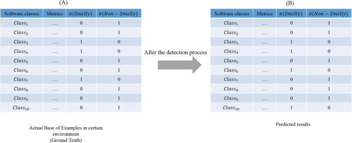

  

  Example of the obtained PBE after the detection process

  A certain PBE includes only one fully possible class label (i.e., its possibility degree is equal to 1) and the remaining class labels are impossible (i.e., their possibility degrees are equal to 0). In this appendix, we demonstrate that the PF-measure_dist working process corresponds to the conventional F-measure one in a certain environment. Figure 19 presents two PBEs (A) and (B), where PBE (A) is the ground truth and PBE (B) is the predicted one. It is important to note that the two PBEs (A) and (B) correspond to the detection process and their labels have the form of possibility distributions. The PF-measure_dist is calculated as follows. First, we start by measuring the closeness between the initial instance (from the ground truth) and the predicted one using sd(I_j) (cf. Equation 10). Then, we normalize the obtained sd(I_j) value using NSD(I_j) (cf. Eq. 11). Finally, based on the comparison between the predicted obtained class labels and the initial ones, we add the obtained NSD(I_j) value to one of these measures: TP_dist (if the actual Smelly classes correctly classified) or FP_dist (if the actual Smelly classes miss-classified as Non-smelly) or TN_dist (if the actual Non-smelly classes correctly classified) or FN_dist (Actual Non-smelly classes miss-classified as Smelly). One can see from Fig. 19 that the possibility distribution value of Class₁ in PBE (A) is similar to the predicted one in PBE (B). The sd(I_j) and NSD(I_j) values of Class₁ are calculated as follows: sd(I₁) = (0 − 0)² + (1 − 1) = 0 and NSD(I₁) = 1. TP_dist= NSD(I₁) +TP_dist, TN_dist= NSD(I₁) +TN_dist, FP_dist= NSD(I₁) +FP_dist, FN_dist= NSD(I₁) +FN_dist ⇒ TP_dist= 0, TN_dist= 1, FP_dist= 0, FN_dist= 0.

  Similarly, sd(I₆) and NSD(I₆) values of Class₆ are calculated as follows:

  sd(I₆) = (1 − 0)² + (0 − 1) = 2 and NSD(I₆) = 1 ⇒ TP_dist= 0, TN_dist= 0, FP_dist= 0, FN_dist= 1. TP_dist= NSD(I₆) +TP_dist, TN_dist= NSD(I₆) +TN_dist, FP_dist= NSD(I₆) +FP_dist, FN_dist= NSD(I₆) +FN_dist

  This process is continued until reaching the final instance. Thus, we will obtain the following values:

  ⇒ TP_dist= 2, TN_dist= 3, FP_dist= 0, FN_dist= 1.

  Based on the obtained values of TP_dist, TN_dist, FP_dist, FN_dist (which are equal to 2, 5, 1, and 2, respectively), we calculate the Precision_dist and Recall_dist values (which are equal to 0.6667 and 0, respectively). These latter are used to compute the PF-measure_dist (PF-measure_dist= 0.571). From this example, one can observe that the calculated PF-measure_dist value is equal to the F-measure one.

• 2. Proof of correspondence between the IAC and the Accuracy: The IAC measure (cf. Equation 16) is based on the distance d (cf. Equation 20) and the Inconsistency Inc (cf. Equation 17) and it is calculated as follows:

  $$ d\left( \pi_{1}^{ini},\pi_{1}^{pred}\right)=\frac{|0-0|+|1-1|}{2}=0 $$
  $$ Inc\left( \pi_{1}^{ini},\pi_{1}^{pred}\right)=1-max(min(0, 0), min(1, 1))=0 $$
  $$ Aff\left( \pi_{1}^{ini},\pi_{1}^{pred}\right)=1-\frac{0.5*0+0.5*0}{1}=1, $$

  where the two parameters κ and λ are set to 0.5. Similarly, d and Inc values of Class₆ are calculated as follows:

  $$ d\left( \pi_{6}^{ini},\pi_{6}^{pred}\right)=\frac{|0-1|+|1-0|}{2}=1 $$
  $$ Inc\left( \pi_{6}^{ini},\pi_{6}^{pred}\right)=1-max(min(0, 1), min(1, 0))=1 $$
  $$ Aff\left( \pi_{6}^{ini},\pi_{6}^{pred}\right)=1-\frac{0.5*1+0.5*1}{1}=0, $$
  $$ d\left( \pi_{6}^{ini},\pi_{6}^{pred}\right)=\frac{|0-0|+|1-1|}{2}=0 $$
  $$ Inc\left( \pi_{6}^{ini},\pi_{6}^{pred}\right)=1-max(min(0, 0), min(1, 1))=0 $$
  $$ Aff\left( \pi_{6}^{ini},\pi_{6}^{pred}\right)=1-\frac{0.5*0+0.5*0}{1}=1 $$

  This process is continued until reaching the final instance. Thus, we will obtain the following values:

  $$ \begin{array}{@{}rcl@{}} && Aff\left( \pi_{1}^{ini},\pi_{1}^{pred}\right)\ =\ 1, \quad Aff\left( \pi_{2}^{ini},\pi_{2}^{pred}\right)\ =\ 1, \quad Aff\left( \pi_{3}^{ini},\pi_{3}^{pred}\right)\ =\ 1, \\ && Aff\left( \pi_{4}^{ini},\pi_{4}^{pred}\right)\ =\ 1, \quad Aff\left( \pi_{5}^{ini},\pi_{5}^{pred}\right)\ =\ 1, \quad Aff\left( \pi_{6}^{ini},\pi_{6}^{pred}\right)\ =\ 0, \\ && Aff\left( \pi_{7}^{ini},\pi_{7}^{pred}\right)\ =\ 0, \quad Aff\left( \pi_{8}^{ini},\pi_{8}^{pred}\right)\ =\ 1, \quad Aff\left( \pi_{9}^{ini},\pi_{9}^{pred}\right)\ =\ 1, \\ && Aff\left( \pi_{10}^{ini},\pi_{10}^{pred}\right)\ =\ 0. \end{array} $$

  ⇒ $IAC=\frac {1}{n}\times {\sum }_{i=1}^{10}Aff\left (\pi _{i}^{ini},\pi _{i}^{pred}\right )=0.7$

  Table 14 AUC median values of ADIPE, DECOR, GP, MOGP, and BLOP for 31 runs of the detection task at the certain environment

  Table 15 AUC median values of ADIPE, DECOR, GP, MOGP, and BLOP for 31 runs of the identification task at the certain environment

  Based on the obtained values of the TP and TN (which are 2 and 5, respectively), the Accuracy value is calculated as follows: $Accuracy=\frac {TP+TN}{Total number of instances}=\frac {2+5}{10}=0.7$ Based on this example, one can conclude that the IAC measure corresponds to the Accuracy measure in a certain environment.

Appendix E: Comparison between ADIPE and the remaining approaches using the AUC and AURPC measures

In this appendix, we present the obtained results of ADIPE, DECOR, GP, MOGP, and BLOP for the detection and identification cases under a certain environment using the AUC (Area Under ROC Curve) metric. In order to ensure a fair comparison, we evaluate the performance of the five compared algorithms in the certain environment since DECOR, GP, MOGP, and BLOP are not conceived to deal with uncertainty. Tables 14 and 15 show the AUC values of the different considered approaches including ADIPE for the detection and identification tasks, respectively. Based on Table 14, one can see that ADIPE surpasses all the considered approaches with an AUC value that lies within [0.9225, 0.9452], while BLOP succeeds to obtain the second-best performance with an AUC value that ranges between 0.1923 and 0.3256. DECOR, GP, and MOGP have a lower performance since their obtained AUC values are equal to 0.114, 0.2382, and 0.2874, respectively. The outperformance of ADIPE could be explained by the fact that its fitness function (i.e., PF-measure_dist) is insensitive to the problem of imbalanced data. GP, MOGP, and BLOP have a lower performance since their fitness functions are not suitable to deal with imbalanced data, which may create ineffective detection rules. DECOR has the lowest AUC values since it is a rule-based algorithm characterized with a set of manually defined detection rules. Table 15 shows similar results for the identification case. The AUC values of ADIPE are slightly degraded, while the AUC values of DECOR, GP, MOGP, and BLOP are significantly degraded due to the high imbalance ratio over the identification process. It should be noted that the A-statistic results are similar to the obtained ones in Tables 6 and 8. Similar results are obtained for the AURPC (Area Under Recall Precision Curve) metric based on Tables 16 and 17. One can observe that ADIPE has the best performance in terms of AURPC in all the considered software projects, while BLOP has the second best performance. This observation clearly demonstrates the ability of our approach to deal with imbalanced data.

Table 16 AURPC median values of ADIPE, DECOR, GP, MOGP, and BLOP for 31 runs of the detection task at the certain environment

Table 17 AURPC median values of ADIPE, DECOR, GP, MOGP, and BLOP for 31 runs of the identification task at the certain environment

Appendix F: Motivations for the Evolutionary design of PDTs

Fig. 20

Illustration of the schema for PDT configuration of two local optima as well as one global optimum search using the PF − measure_dist

In this appendix, we highlight the advantages of using EAs in optimizing PDTs. In the literature, machine learning algorithms have been widely used in designing PDTs (Barros et al. 2012; Al-Sahaf et al. 2019). However, existing machine learning algorithms could lead the solution to got stack into local optima. One of the well-known EAs is the GA that has proven its ability to escape from local optima (Holland 1992). Figure 20 illustrates the schema for PDT configuration of two local optima as well as one global optimum search using the PF − measure_dist. Each point on the x-axis represents a PDT configuration for ease of visualization, while the y-axis displays the value of the PF − measure_dist (configuration quality). According to this schema, starting with solution (configuration) A, the greedy algorithm will converge to one of the two globally optimal PDT structures G₁ or G₂. Likewise, if it begins induction with solution B, it could approximate the global optimum G₃ or the local one G₂. As a result, the chance that a greedy PDT induction method finding a closer globally-optimal configuration is extremely low, whereas GAs do not have this problem due to two features. From one side, similarly to any EA approach, the GA has a global search capability because it can identify promising regions within the search space, more precisely,regions close to G₁, G₂, and G₃. This could be done by simultaneously evolving up an entire population (a number of configurations) rather than just a single configuration. On the other side, the binary tournament operator allows the acceptance of poor configurations (PF − measure_dist degradation). Based on this fact, the GA can avoid falling into local optima like solutions close to G₁ and G₂. Such operator carries out (N/2) iterations to pick up (N/2) offsprings for the reproduction process. Accordingly, when two PDT configurations are chosen from the mating pool as parents for crossover, these parents could include both good and bad PDT configurations. As a result, the GA permits the fitness function to deteriorate, allowing it to: (1) avoid local optima like solution G₂ and then (2) guide the search process through the globally optimal PDT configuration G₃. Another reason for the employment of the GA algorithm is that it has shown good performance in the certain environment (Boutaib et al. 2020). Motivated by the mentioned advantages of the GA, we have proposed to assess its performance over the uncertain environment.

Appendix G: Comparison based on the CPU time between the peer algorithms

In this Appendix, we compare the considered algorithms in our experimental study (i.e., GP, MOGP, BLOP, and ADIPE) from the CPU time viewpoint. In fact, all the algorithms under comparison were executed on machines with Intel Core i7 2.20 GHz processor and 8 GB RAM. We also note that we have used the simplest pseudo-parallel approach, which is the multi-threading. Table 18 shows the CPU times obtained in each software project for each induction algorithm (i.e., GP, MOGP, BLOP, and ADIPE). For fairness of comparison, we use the same number of evaluation for all the considered algorithms. This stopping criterion is set to 256,500 for all the used software projects. One can see from Table 18 that the CPU time consumed by ADIPE is higher than the ones of GP, MOGP, and BLOP since the update procedure of the reproduction operators, the building structure of our PDT, and the evaluation process are a little time consuming. Table 19 reports the CPU times obtained by PDT ensemble, DECOR, GP-Tree, MOGP-Tree, and BLOP-Tree on the unseen project (i.e., Lucene v1.4.1¹⁴ with 154 software classes and 41 smells). One can observe from Table 19 that the CPU time of ADIPE is slightly higher than the ones of its competitors since it uses a PDT ensemble instead of a single detector, which is the case of the other approaches.

Table 18 CPU time consumed in hours by GP, MOGP, BLOP, and ADIPE on the six considered software projects (i.e., GanttProject, ArgoUML, Xercess-J, JFreeChart, Apache Ant, Azureus)

Table 19 CPU time consumed in milliseconds by DECOR, GP-Tree, MOGP-Tree, BLOP-Tree, and PDT ensemble on the unseen project Lucene v1.4.1

Appendix H: Investigation of ADIPE performance on a cross-project

Fig. 21

Illustration of the application of the PDT ensemble on a cross-project problem

Table 20 PF-measure_dist and IAC (F-measure and Accuracy) median scores of ADIPE, DECOR, GP, MOGP, and BLOP for 31 runs of the detection task at the uncertain (and certain ) environments on the Lucene v1.4.1 unseen project

In this appendix, we show how the proposed approach is able to achieve good performance on cross-projects code smell detection. As shown in Fig. 21, ADIPE is trained based on the source projects that have been used to construct the PBE. In an industrial context, these software projects are labeled by software engineers that may have some uncertainty and doubtfulness regarding the smelliness of a number of software classes. The output of ADIPE is a PDT ensemble that are applied to the target project that is not considered in the training process. It is important to note that before the application of the PDT ensemble, a TCA (Transfer Component Analysis) (Pan et al. 2010) method is used as a Domain Adaptation module. This latter aims to have similar distributions between the source projects and the target one, since having different distributions between the source and target projects may have a negative influence on the performance of the classifiers. After the application of the Domain Adaptation module, the PDTs could be applied to predict the labels of the existing smelly instances of the target project. Therefore, the uncertainty of the software engineers are transferred from the source projects to the target ones through the application of the PDT detectors (PDT ensemble). In the validation step, the software engineers label the software classes of the target project to be able to compare it with the predicted software class labels obtained by the PDT detectors. It is worth noting that the labeling step is performed by the same software engineers that have constructed the BE of the source projects. An important threat that should not be ignored is that the validation of the results must be performed by the developers who developed the Lucene software project and not those who built the base of examples. Hence, since the training step, the environment nature (certain or uncertain) of the source and target projects is specified based on the opinions of the software engineers. This validation process allows us to evaluate the effectiveness of the constructed PDTs in transferring the uncertainty of the human experts when introducing unseen software cross-projects. In this appendix, we have investigated the performance of our approach on the unseen Lucene 1.4.1 software project using the PF-measure_dist and IAC measures in the uncertain environment and the F-measure and the Accuracy in the certain one. Table 20 shows that ADIPE outperforms the remaining approaches (DECOR, GP, MOGP, and BLOP) in both environments with respect to all the considered metrics. ADIPE achieves 0.9115 and 0.9273 in terms of PF-measure_dist and IAC, respectively. The second best performance is obtained by BLOP where it succeeds to obtain 0.2183 and 0.2330 in terms of PF-measure_dist and IAC measures. The same performance is obtained by the compared algorithms in the certain environment.

References

Al-Sahaf H, Bi Y, Chen Q, Lensen A, Mei Y, Sun Y, Tran B, Xue B, Zhang M (2019) A survey on evolutionary machine learning. J R Soc N Z 49(2):205–228
Alcalá-Fdez J, Fernández A, Luengo J, Derrac J, García S, Sánchez L, Herrera F (2011) Keel data-mining software tool: data set repository, integration of algorithms and experimental analysis framework. J Multiple-Valued Log Soft Comput 17
Amorim L, Costa E, Antunes N, Fonseca B, Ribeiro M (2015) Experience report: Evaluating the effectiveness of decision trees for detecting code smells. In: Proceedings of the 26th International Symposium on Software Reliability Engineering,. IEEE, pp 261–269
Arcuri A, Briand L (2014) A Hitchhiker’s guide to statistical tests for assessing randomized algorithms in software engineering. Softw Test Verif Reliab 24 (3):219–250
Azeem M I, Palomba F, Shi L, Wang Q (2019) Machine Learning Techniques for Code Smell Detection: A Systematic Literature Review and Meta-Analysis. Inf Softw Technol 108:115–138
Barbez A, Khomh F, Guéhéneuc Y-G (2019) Deep learning anti-patterns from code metrics history. In: Proceedings of the IEEE International Conference on Software Maintenance and Evolution (ICSME 2019). IEEE, pp 114–124
Barros R C, Basgalupp M P, De Carvalho A C, Freitas A A (2012) A survey of evolutionary algorithms for decision-tree induction. IEEE Trans Syst Man Cybern 42(3):291–312
Behmo R, Marcombes P, Dalalyan A, Prinet V (2010) Towards optimal naive bayes nearest neighbor. In: European conference on computer vision. Springer, pp 171–184
Bessghaier N, Ouni A, Mkaouer M W (2020) On the diffusion and impact of code smells in web applications. In: International Conference on Services Computing. Springer, pp 67–84
Bouchon-Meunier B, Dubois D, Godo L, Prade H (1999) Fuzzy sets in approximate reasoning and information systems, vol 5. Kluwer Academic Publishers
Bounhas M, Hamed M G, Prade H, Serrurier M, Mellouli K (2014) Naive possibilistic classifiers for imprecise or uncertain numerical data. Fuzzy Sets Syst 239:137–156
Boussaa M, Kessentini W, Kessentini M, Bechikh S, Chikha S B (2013) Competitive Coevolutionary Code-Smells Detection. In: Proceedings of the 5th International Symposium on Search Based Software Engineering, vol 8084. Springer, pp 50–65
Boussaïd I, Siarry P, Ahmed-Nacer M (2017) A survey on search-based model-driven engineering. Autom Softw Eng 24:233–294
Boutaib S, Bechikh S, Palomba F, Elarbi M, Makhlouf M, Said L B (2020) Code smell detection and identification in imbalanced environments. Expert Syst Appl 166:114076
Boutaib S, Elarbi M, Bechikh S, Hung C-C, Said L B (2021) Software anti-patterns detection under uncertainty using a possibilistic evolutionary approach.. In: EuroGP, pp 181–197
Bowers K M, Fredericks E M, Hariri R H, Cheng B H (2020) Providentia: Using search-based heuristics to optimize satisficement and competing concerns between functional and non-functional objectives in self-adaptive systems. J Syst Softw 162:1–51
Brindle A (1980) Genetic algorithms for function optimization. Ph.D. Thesis, The Faculty of Graduate Studies University of Alberta
Conover W J, Conover W J (1980) Practical nonparametric statistics. Wiley, New York
de Paulo Sobrinho E V, De Lucia A, de Almeida Maia M (2018) A systematic literature review on bad smells—5 w’s: which, when, what, who, where. IEEE Trans Softw Eng
Dhambri K, Sahraoui H, Poulin P (2008) Visual detection of design anomalies. In: Proceedings of the 12th European Conference on Software Maintenance and Reengineering,. IEEE, pp 279–283
Di Nucci D, Palomba F, Tamburri D A, Serebrenik A, De Lucia A (2018) Detecting code smells using machine learning techniques: are we there yet?. In: Proceedings of the 25th International Conference on Software Analysis, Evolution and Reengineering. IEEE, pp 612–621
Du X, Zhou Z, Yin B, Xiao G (2019) Cross-project bug type prediction based on transfer learning. Softw Qual J:1–19
Dubois D, Prade H (1988) Possibility theory: an approach to computerized processing of uncertainty
Dubois D, Prade H (1985) Unfair coins and necessity measures: towards a possibilistic interpretation of histograms. Fuzzy Sets Syst 10(1-3):15–20
Dubois D, Prade H (1994) La fusion d’informations imprécises. Traitement Signal 11(6):447–458
Dubois D, Prade H (1994) Possibility theory and data fusion in poorly informed environments. Control Eng Pract 2(5):811–823
Dubois D, Prade H (2000) Possibility theory in information fusion. In: Proceedings of the 3rd international conference on information fusion, vol 1. IEEE, pp 6–P19
Dunford N, Schwartz JT, WG B, RG B (1971) Linear operators. Wiley-Interscience, New York
Eiben A E, Smit S K (2011) Parameter tuning for configuring and analyzing evolutionary algorithms. Swarm Evol Comput 1(1):19–31
Emden E V, Moonen L (2002) Java quality assurance by detecting code smells. In: Proceedings of the 9th Working Conference on Reverse Engineering. IEEE, pp 97–106
Erni K, Lewerentz C (1996) Applying design-metrics to object-oriented frameworks. In: Proceedings of the 3rd international software metrics symposium. IEEE, pp 64–74
Fernandes E, Oliveira J, Vale G, Paiva T, Figueiredo E (2016) A review-based comparative study of bad smell detection tools. In: Proceedings of the 20th Conference on Evaluation and Assessment in Software Engineering. ACM, p 18
Fontana F A, Braione P, Zanoni M (2012) Automatic detection of bad smells in code: An experimental assessment. J Object Technol 11(2):5–1
Fontana F A, Dietrich J, Walter B, Yamashita A, Zanoni M (2016) Antipattern and code smell false positives: Preliminary conceptualization and classification. In: 2016 IEEE 23rd international conference on software analysis, evolution, and reengineering (SANER), vol 1. IEEE, pp 609–613
Fontana F A, Mäntylä M V, Zanoni M, Marino A (2016) Comparing and experimenting machine learning techniques for code smell detection. Empir Softw Eng 21(3):1143–1191
Fontana F A, Zanoni M (2017) Code smell severity classification using machine learning techniques. Knowl-Based Syst 128:43–58
Foundation A S (2004) Apache commons cli. http://commons.apache.org/cli/ [Accessed 19-April-2021]
Fowler M, Beck K (1999) Refactoring: improving the design of existing code. Addison-Wesely
Friedman N, Geiger D, Goldszmidt M (1997) Bayesian network classifiers. Mach Learn 29(2-3):131–163
Fu S, Shen B (2015) Code Bad Smell Detection through Evolutionary Data Mining. In: Proceedings of the ACM/IEEE International Symposium on Empirical Software Engineering and Measurement. IEEE, pp 1–9
Gopalan R (2012) Automatic detection of code smells in java source code. Ph.D. Thesis, University of Western Australia
Hadj-Kacem M, Bouassida N (2019) Deep representation learning for code smells detection using variational auto-encoder. In: Proceedings of the International Joint Conference on Neural Networks (IJCNN). IEEE, pp 1–8
Hassaine S, Khomh F, Guéhéneuc Y-G, Hamel S (2010) IDS: An immune-inspired approach for the detection of software design smells. In: Proceedings of the 7th International Conference on Quality of Information and Communications Technology. IEEE, pp 343–348
Henderson-Sellers B (1995) Object-oriented metrics: measures of complexity. Prentice-Hall, Inc.
Higashi M, Klir G J (1983) On the notion of distance representing information closeness: Possibility and probability distributions. Int J Gen Syst 9 (2):103–115
Holland J H (1992) Genetic algorithms. Sci Amer 267(1):66–73
Holmes C, Adams N (2002) A probabilistic nearest neighbour method for statistical pattern recognition. J R Stat Soc Ser B (Stat Methodol) 64 (2):295–306
Hosseini S, Turhan B, Mäntylä M (2018) A benchmark study on the effectiveness of search-based data selection and feature selection for cross project defect prediction. Inf Softw Technol 95:1–17
Jenhani I (2010) From possibilistic similarity measures to possibilistic decision trees. Ph.D. Thesis, Artois
Jenhani I, Amor N B, Benferhat S, Elouedi Z (2008) Sim-pdt: A similarity based possibilistic decision tree approach. In: Proceedings of the International Symposium on Foundations of Information and Knowledge Systems. Springer, pp 348–364
Jenhani I, Amor N B, Elouedi Z (2008) Decision trees as possibilistic classifiers. Int J Approx Reason 48(3):784–807
Jenhani I, Amor N B, Elouedi Z, Benferhat S, Mellouli K (2007) Information affinity: A new similarity measure for possibilistic uncertain information. In: Proceedings of the European Conference on Symbolic and Quantitative Approaches to Reasoning and Uncertainty. Springer, pp 840–852
Jenhani I, Benferhat S, Elouedi Z (2009) On the use of clustering in possibilistic decision tree induction. In: Proceedings of the European Conference on Symbolic and Quantitative Approaches to Reasoning and Uncertainty. Springer, pp 505–517
Karafotias G, Hoogendoorn M, Eiben A E (2015) Parameter control in evolutionary algorithms: Trends and challenges. IEEE Trans Evol Comput 19:167–187
Kessentini M, Sahraoui H, Boukadoum M, Wimmer M (2011) Search-Based Design Defects Detection by Example. In: Proceedings of the 14th International Conference on Fundamental Approaches to Software Engineering, vol 6603. Springer, pp 401–415
Kessentini W, Kessentini M, Sahraoui H, Bechikh S, Ouni A (2014) A Cooperative Parallel Search-Based Software Engineering Approach for Code-Smells Detection. IEEE Trans Softw Eng 40(9):841–861
Khomh F, Vaucher S, Guéhéneuc Y-G, Sahraoui H (2009) A bayesian approach for the detection of code and design smells. In: Proceedings of the 9th International Conference on Quality Software. IEEE, pp 305–314
Khomh F, Vaucher S, Guéhéneuc Y-G, Sahraoui H (2011) BDTEX: A GQM-based Bayesian approach for the detection of antipatterns. J Syst Softw 84(4):559–572
Klement E P, Mesiar R, Pap E (2000) Triangular norms
Kreimer J (2005) Adaptive detection of design flaws. Electron Notes Theor Comput Sci 141(4):117–136
Krętowski M, Grześ M (2005) Global learning of decision trees by an evolutionary algorithm. In: Information Processing and Security Systems. Springer, pp 401–410
Kroupa T (2006) Application of the choquet integral to measures of information in possibility theory. Int J Intell Syst 21(3):349–359
Langelier G, Sahraoui H, Poulin P (2005) Visualization-based analysis of quality for large-scale software systems. In: Proceedings of the 20th IEEE/ACM international Conference on Automated software engineering. ACM, pp 214–223
Lanza M, Marinescu R (2007) Object-oriented metrics in practice: using software metrics to characterize, evaluate, and improve the design of object-oriented systems. Springer Science & Business Media
Li K, Xiang Z, Chen T, Tan K C (2020) Bilo-cpdp: Bi-level programming for automated model discovery in cross-project defect prediction. In: 2020 35th IEEE/ACM International Conference on Automated Software Engineering (ASE). IEEE, pp 573–584
Liu H, Jin J, Xu Z, Bu Y, Zou Y, Zhang L (2019) Deep learning based code smell detection. IEEE Trans Softw Eng
Ma C Y, Wang X Z (2009) Inductive data mining based on genetic programming: Automatic generation of decision trees from data for process historical data analysis. Comput Chem Eng 33(10):1602–1616
Maiga A, Ali N, Bhattacharya N, Sabane A, Gueheneuc Y-G, Aimeur E (2012a) SMURF: A SVM-based incremental anti-pattern detection approach. In: Proceedings of the 19th Working conference on Reverse engineering,. IEEE, pp 466–475
Maiga A, Ali N, Bhattacharya N, Sabané A, Guéhéneuc Y-G, Antoniol G, Aïmeur E (2012b) Support vector machines for anti-pattern detection. In: Proceedings of the 27th IEEE/ACM International Conference on Automated Software Engineering. IEEE, pp 278–281
Mansoor U, Kessentini M, Bechikh S, Deb K (2013) Code-smells detection using good and bad software design examples. Technical report, Technical Report
Mansoor U, Kessentini M, Maxim B R, Deb K (2017) Multi-objective code-smells detection using good and bad design examples. Softw Qual J 25(2):529–552
Mantyla M V, Vanhanen J, Lassenius C (2004) Bad smells-humans as code critics. In: 20th IEEE International Conference on Software Maintenance, 2004. Proceedings. IEEE, pp 399–408
Marinescu R (2002) Measurement and quality in object oriented design. Ph.D. Thesis, Politehnica University of Timisoara
Marinescu R (2004) Detection strategies: Metrics-based rules for detecting design flaws. In: Proceedings of the 20th IEEE International Conference on Software Maintenance. IEEE, pp 350–359
Martin R C (2002) Agile software development: principles, patterns, and practices. Prentice Hall
Moha N, Gueheneuc Y G, Duchien L, Meur A F L (2010) DECOR: A Method for the Specification and Detection of Code and Design Smells. IEEE Trans Softw Eng 36(1):20–36
Oliveto R, Khomh F, Antoniol G, Guéhéneuc Y-G (2010) Numerical signatures of antipatterns: An approach based on b-splines. In: Proceedings of the 14th European Conference on Software maintenance and reengineering. IEEE, pp 248–251
Ouni A (2014) A mono-and multi-objective approach for recommending software refactoring. Ph.D. Thesis, Faculty of arts and sciences of Montreal
Ouni A, Kessentini M, Sahraoui H, Boukadoum M (2013) Maintainability defects detection and correction: a multi-objective approach. Autom Softw Eng 20(1):47–79
Palomba F, Bavota G, Di Penta M, Oliveto R, De Lucia A (2014) Do they really smell bad? a study on developers’ perception of bad code smells. In: 2014 IEEE International Conference on Software Maintenance and Evolution. IEEE, pp 101–110
Palomba F, Bavota G, Di Penta M, Oliveto R, Poshyvanyk D, De Lucia A (2015) Mining version histories for detecting code smells. IEEE Trans Softw Eng 41(5):462–489
Palomba F, Bavota G, Penta M D, Oliveto R, Lucia A D, Poshyvanyk D (2013) Detecting bad smells in source code using change history information. In: Proceedings of the 28th IEEE/ACM International Conference on Automated Software Engineering. IEEE Press, pp 268–278
Palomba F, Panichella A, Zaidman A, Oliveto R, De Lucia A (2017) The scent of a smell: An extensive comparison between textual and structural smells. IEEE Trans Softw Eng 44(10):977–1000
Pan S J, Tsang I W, Kwok J T, Yang Q (2010) Domain adaptation via transfer component analysis. IEEE Trans Neural Netw 22(2):199–210
Pearl J (1982) Reverend bayes on inference engines: A distributed hierarchical approach. In: Proceedings of the Second AAAI Conference on Artificial Intelligence. AAAI Press, pp 133–136
Pearl J (1985) Bayesian netwcrks: A model cf self-activated memory for evidential reasoning. In: Proceedings of the 7th Conference of the Cognitive Science Society. University of California, Irvine, pp 15–17
Pecorelli F, Di Nucci D, De Roover C, De Lucia A (2020) A large empirical assessment of the role of data balancing in machine-learning-based code smell detection. J Syst Softw:110693
Pecorelli F, Palomba F, Di Nucci D, De Lucia A (2019) Comparing Heuristic and Machine Learning Approaches for Metric-Based Code Smell Detection. In: Proceedings of the IEEE/ACM International Conference on Program Comprehension. IEEE, p 12
Pecorelli F, Palomba F, Khomh F, De Lucia A (2020) Developer-driven code smell prioritization. In: Proceedings of the 17th International Conference on Mining Software Repositories, pp 220–231
Qing H, Biwen L, Beijun S, Xia Y (2015) Cross-project software defect prediction using feature-based transfer learning. In: Proceedings of the 7th Asia-Pacific Symposium on Internetware, pp 74–82
Quinlan J R (1987) Decision trees as probabilistic classifiers. In: Proceedings of the Fourth International Workshop on Machine Learning. Elsevier, pp 31–37
Ramirez A, Romero J R, Ventura S (2018) A survey of many-objective optimisation in search-based software engineering. J Syst Softw 149:382–395
Rapu D, Ducasse S, Gîrba T, Marinescu R (2004) Using history information to improve design flaws detection. In: Proceedings of the 8th European Conference on Software Maintenance and Reengineering,. IEEE, pp 223–232
Sahin D, Kessentini M, Bechikh S, Deb K (2014) Code-Smell Detection as a Bilevel Problem. ACM Trans Softw Eng Methodol 24(1):1–44
Saidani I, Ouni A, Mkaouer M W (2020) Web service api anti-patterns detection as a multi-label learning problem. In: International Conference on Web Services. Springer, pp 114–132
Sangüesa R, Cabós J, Cortes U (1998) Possibilistic conditional independence: A similarity-based measure and its application to causal network learning. Int J Approx Reason 18(1-2):145–167
Sharma T, Spinellis D (2018) A survey on software smells. J Syst Softw 138:158–173
Taibi D, Janes A, Lenarduzzi V (2017) How developers perceive smells in source code: A replicated study. Inf Softw Technol 92:223–235
Tsang S, Kao B, Yip K Y, Ho W-S, Lee S D (2009) Decision trees for uncertain data. IEEE Trans Knowl Data Eng 23(1):64–78
Tsantalis N, Chatzigeorgiou A (2009) Identification of Move Method Refactoring Opportunities. IEEE Trans Softw Eng 35(3):347–367
Tsantalis N, Chatzigeorgiou A (2011) Identification of extract method refactoring opportunities for the decomposition of methods. J Syst Softw 84:1757–1782
Tufano M, Palomba F, Bavota G, Oliveto R, Di Penta M, De Lucia A, Poshyvanyk D (2017) When and why your code starts to smell bad (and whether the smells go away). IEEE Trans Softw Eng 43(11):1063–1088
Van Rijsbergen CJ (1979) Information retrieval
Vargha A, Delaney H D (2000) A critique and improvement of the cl common language effect size statistics of mcgraw and wong. J Educ Behav Stat 25 (2):101–132
Vaucher S, Khomh F, Moha N, Guéhéneuc Y-G (2009) Tracking design smells: Lessons from a study of god classes. In: Proceedings of the 16th Working Conference on Reverse Engineering,. IEEE, pp 145–154
Whittle J, Sawyer P, Bencomo N, Cheng B H, Bruel J-M (2009) Relax: Incorporating uncertainty into the specification of self-adaptive systems. In: Proceedings of the 17th International Requirements Engineering Conference. IEEE, pp 79–88
Wirfs-Brock R, McKean A (2003) Object design: roles, responsibilities, and collaborations. Addison-Wesley Professional
Yamashita A, Moonen L (2013) Do developers care about code smells? an exploratory survey. In: 2013 20th Working Conference on Reverse Engineering (WCRE). IEEE, pp 242–251
Zadeh L A (1978) Fuzzy sets as a basis for a theory of possibility. Fuzzy Sets Syst 1(1):3–28
Zhu Z, Li Y, Tong H, Wang Y (2020) Cooba: Cross-project bug localization via adversarial transfer learning. In: Proceedings of the Twenty-Ninth International Joint Conference on Artificial Intelligence, IJCAI, pp 3565–3571
Zimmermann T, Nagappan N, Gall H, Giger E, Murphy B (2009) Cross-project defect prediction: a large scale experiment on data vs. domain vs. process. In: Proceedings of the 7th joint meeting of the European software engineering conference and the ACM SIGSOFT symposium on The foundations of software engineering, pp 91–100
Acknowledgements
Fabio Palomba gratefully acknowledges the support of the Swiss National Science Foundation through the SNF Project No. PZ00P2_186090 (TED).
Author information
Authors and Affiliations
Corresponding authors
Ethics declarations
Conflict of interest
The authors declare that they have no known competing interests or personal relationships that could have appeared to influence the work reported in this paper.
Additional information
Communicated by: Federica Sarro
Publisher’s note
Springer Nature remains neutral with regard to jurisdictional claims in published maps and institutional affiliations.