Deep cross-platform product matching in e-commerce

Abstract

Online shopping has become more and more popular in recent years, which leads to a prosperity on online platforms. Generally, the identical products are provided by many sellers on multiple platforms. Thus the comparison between products on multiple platforms becomes a basic demand for both consumers and sellers. However, identifying identical products on multiple platforms is difficult because the description for a certain product can be various. In this work, we propose a novel neural matching model to solve this problem. Two kinds of descriptions (i.e. product titles and attributes), which are widely provided on online platforms, are considered in our method. We conduct experiments on a real-world data set which contains thousands of products on two online e-commerce platforms. The experimental results show that our method can take use of the product information contained in both titles and attributes and significantly outperform the state-of-the-art matching models.

1 Introduction

With the development of Internet and mobile technologies, online shopping becomes more and more popular. Massive offline transactions have been moved to online which leads to a prosperity on online platforms such as Amazon, eBay, Tmall, and JD. As different consumers prefer different platforms, it is common for sellers to sell their products on multiple online platforms simultaneously. For consumers, purchasing a product from a certain platform is usually decided based on the comparison of prices, qualities, and users’ feedbacks (comments). For example, consumers tend to choose the cheapest one if identical products are offered on multiple platforms. When both price and quality are analogous, they prefer the one offered by a seller with better service. Meanwhile, comparing their products with competitors is an effective way to do pricing and sales strategy adjustment for both sellers and platform managers. Therefore, it is valuable to study the problem of identifying identical products on different platforms.

Fig. 1

An example of three products sold on two platforms. Product a is sold on Tmall, while product b and c are sold on JD. The text in gray background is product title and product attributes are listed under it. In this example, a and b are identical products, while a and c are different. There are synonyms in product attribute names. The last attribute name Effect in b and the last attribute name Function in a represent the same meaning

On online e-commerce platforms, products usually described by their product titles and product attributes. A product title usually contains the key information about this product, and it is generally a brief and free text. Attributes are provided to specify more details about products, and they are usually in the format of name-value pairs from catalog data or from structured tables on web pages. Let us use an actual example (showed in Fig. 1) to demonstrate it. In Fig. 1, the title of product (a) is Head and Shoulders Anti-Dandruff Shampoo (Fresh and Oil Control) 750 ml, which refers to a kind of shampoo made by Head and Shoulders. In addition to the brand name, this title also contains information about the net weight and other main product specifications. Moreover, the attributes of product (a) include Place of Origin: Mainland China and N.W.: 750 ml, etc. The examples in Fig. 1 are sampled from two online platforms Tmall and JD. And these products are also provided by other online platforms such as Amazon and eBay. Both titles and attributes are useful for identifying identical products. However, given the titles and attributes of two products, it is still difficult to identify whether they are identical or not. One difficulty is that products are described in different manners according to sellers’ demands and the format of titles and attributes is different. As illustrated in Fig. 1, (a) and (b) are the same products sold on two platforms, but their titles and attributes are different. Another difficulty of product matching is the synonyms. Synonyms not only appear in product titles, but also appear in product attributes. As illustrated in Fig. 1, the last attributes of product (a) and (b) are Function and Effect, but they represent the same meaning substantially. Therefore, how to match products by considering both titles and attributes simultaneously is very challenging.

To tackle aforementioned two difficulties, we propose to make use of product titles and attributes respectively, rather than fusing titles and attributes into documents by simple processing. We design a neural product matching model to judge whether two products are matched and identical. Given two products’ descriptions, for each product title, we use a bidirectional long short term memory network (Bi-LSTM) to generate their representations. Then convolutional neural network (CNN) is introduced to extract features for matching. This structure is inspired by some state-of-the-art models on text matching. Bi-LSTM is proved to be useful in extracting positional information (Schuster and Paliwal 1997), while CNN can be utilized to model the similarities between words in similar positions (Shen et al. 2014; Hu et al. 2014; Pang et al. 2016). We call this module Title Matching Module (TMM shortly). As for attributes, they are usually represented as name-value pairs. Note that the aforementioned structure of TMM is not applicable for attribute matching due to their different formats. So we design an Attributes Matching Module (AMM shortly). The attribute names and values are taken into account respectively and two interaction matrices are built on them in this module. A special convolution operation is used to extract matching features from the interaction matrix of attribute values, and a K-Max pooling operation is used to extract the strongest features from the interaction matrix of attribute names. Then the matching features on attributes are combined together. Consequently, the outputs of TMM and AMM are matching features excerpted from product titles and attributes respectively, and we further fuse them by multi-layer perceptron (MLP) to generate final matching features. The uniform model is named as Product Matching Model (PMM shortly).

To evaluate our model, we simulate two real application scenarios. The first one is identifying if two products are identical when given their titles and attributes. This simulates the scenario that a consumer selects two products to compare. Under this circumstance, only two products are considered, so the task can be categorized as a classification problem. The second application scenario is more complex: one product is provided as a query product and a number of products are given as candidates. The target is to rank the candidate product list according to their similarities with the query product. This scenario aims at simulating behaviors of the sellers and platforms when they use their own products as query products to retrieve similar products on another platform. We conduct experiments on a data set containing about 20 product categories from two real online platforms. The experimental results show that our model outperforms state-of-the-art models in both application scenarios.

To summarize, our contributions are as follows:

• 1. To our best knowledge, we are the first to investigate product matching problem based on both product title and attributes of products. We design a novel model that makes use of the information contained in titles and attributes respectively. The experimental results prove the effectiveness of our model.

• 2. We evaluate our model in two typical application scenarios: a classification scenario and a ranking scenario. Both applications are designed by simulating behaviors of consumers, sellers and platforms when comparing products on two platforms. The results show that our model can work well in both scenarios.

2 Related work

In this section, we introduce the related work in two categories. The first category includes methods proposed for product matching problem. We use similar product descriptive information but our methods are apparently different. The second group of related work is about text matching task. These methods can be extended to product matching problem by considering only product titles or considering both titles and attributes.

2.1 Algorithms for product matching

A number of methods have been proposed for product matching problems. At first, product resolution is a common task for product search engines. In this task, product queries are given by users to search for product entities. Product entities usually include product titles, product attributes, or product reviews. The matching is conducted between users’ queries and product entities. Duan et al. (2013) propose a language modeling approach to optimize search over structured product entities in databases with keyword queries. This approach is suitable for users who are not familiar with SQL language. Duan and Zhai (2015) propose a novel language model to represent users’ intent by capturing both query terms and structured product entities. Van Gysel et al. (2016) introduce a novel latent vector space model that jointly learns unsupervised representations of queries, product entities and the mapping between them. These matching approaches are made between textual queries and products. However, they cannot deal with product matching problem directly since the matching process is made between users’ queries and product entities, rather than between product entities. Things are much more difficult when matching products across platforms. To tackle this problem, many methods have been proposed including record linkage, duplicate detection and entity resolution (Winkler 1999, 2006; Fellegi and Sunter 1969; Christen 2012; Nauman and Herschel 2010).

In fact, on real online platforms, product descriptions typically include product titles and attributes, and they are free data rather than structured data. In the early stage, Kannan et al. (2011) attempt to convert product offers into structured product specifications, and match them with structured data stored in databases, then utilize the aforementioned methods on databases for product matching. Thereafter, researchers gradually pay more attention to match two products based on their descriptions directly. Gopalakrishnan et al. (2012) propose to match two products by their titles, they use a web search engine to assign different weights for words in titles and match them based on weighted word similarities. Köpcke et al. (2012) take a step further to utilize both product titles and attributes to identify identical products, but they only extracted features from descriptions to train a matching model where semantic information is lost.

Our model is distinguished with these existing methods in two aspects: (1) No database in involved. Product titles and attributes are free data without constraints of database structures. (2) Product titles and the corresponding attributes are processed separately by two modules according to their different forms. Their matching features are fused together to generate final product matching score.

2.2 Text matching approaches

Many tasks in natural language processing, such as information retrieval, automatic question answering, machine translation, dialogue system, and repetition, can be categorized into text matching problems. A large number of text matching methods based on deep learning have been proposed. Different tasks owe different matching targets. The information retrieval task is to calculate the matching scores between given queries and documents, and some literature reviews introduce the current landscape of Neural IR research (Mitra and Craswell 2018; Onal et al. 2018). The automatic question answering task is to judge whether an answer is for the given question. Here, the target of our product matching task is to determine whether two products are identical based their product titles and attributes.

When using product titles or both titles and attributes by concatenating them into text instances to match, models proposed for text matching can be applied to the product matching problem. Therefore, some text matching methods are involved as related work. It is worth noting that we only introduce neural network-based models on text matching that are comparable with our model. These models can be roughly categorized into two groups: representation-based methods and interaction-based methods.

Representation-based methods commit to obtain better representations for each text, which is basis for further matching. The state-of-the-art models include DSSM (Huang et al. 2013), CDSSM (Shen et al. 2014), ARC-I (Hu et al. 2014), CNTN (Qiu and Huang 2015) and MV-LSTM (Wan et al. 2016). DSSM is one of the earliest deep models in text matching. Each text is vectorized separately by a five-layer network, and cosine similarity is used to calculate the similarity between two text segments. Compared with DSSM, CDSSM replaces the full connection layer with a convolution layer and a pooling layer to generate text vectors. ARC-I uses convolution operations to represent two texts, and the representations of two texts are concatenated and further used for matching by a linear transformation. CNTN also adopts convolution neural network to represent two texts, and it proposes the neural tensor network to model the similarities between two texts. MV-LSTM uses Bi-LSTM to obtain representation for each text and adopts interaction methods to measure similarities between any two texts, then applies a K-Max pooling strategy to get matching features.

Unlike representation-based approaches, interaction-based approaches usually build an interaction matrix between two texts, and focus on extracting useful information from the interaction matrix for matching. Typical models include ARC-II (Hu et al. 2014), MatchPyramid (Pang et al. 2016), DRMM (Guo et al. 2016), DUET (Mitra et al. 2017) and KNRM (Xiong et al. 2017). ARC-II first builds an interaction matrix, then conducts several convolution and pooling operations to extract matching features. MatchPyramid also first builds an interaction matrix, and uses hierarchical convolution and pooling to capture matching patterns. DRMM also builds an interaction matrix and transforms it into a fixed-length matching histogram to obtain matching degree for each word in queries, and it considers the weights and matching degree of words in queries to generate final matching score. DUET considers both distributed representations and local representations to build distributed model and local model, and obtains final matching score based the two models. KNRM also first builds translation matrix, then adopts kernel-pooling technique to extract soft matching features. Some of aforementioned models, including DSSM, CDSSM, DRMM, DUET and KNRM, are designed specifically for information retrieval tasks. And we select some baselines from these classical text matching models according to their performance on our early experiments.

When regarding product title and attributes as semi-structured document, product matching problem is similar with multiple-field document retrieval task, in which documents are ranked by measuring similarities between user queries and semi-structured documents. NRM-F (Zamani et al. 2018) is a neural matching model proposed specially for multiple-field document retrieval, which models the representations of queries and documents with multiple fields, then measures similarities by the interaction of their representations. Due to the similarity of the two tasks, we extend NRM-F to work with product titles and attributes by regarding products as documents with multiple fields.

3 Product matching model

In this Sect., we introduce our Product Matching Model (PMM shortly). PMM consists of a product title matching module (TMM shortly) and a product attributes matching module (AMM shortly). Before introducing our model, we formally define the product matching problem. Then we present the structure of PMM. And its two sub modules, i.e., TMM and AMM are described respectively in detail thereafter.

3.1 Problem definition

As illustrated in Fig. 2, assuming two products X and Y, the title of X is represented by a sequence of words $(x_1, x_2, \ldots , x_m)$, where $x_i$ is the ith word in the title and m is the title length. The attributes are denoted as a set of name-value pairs, i.e., $\{(k_1: v_1), \ldots , (k_p: v_p) \}$, where $(k_j: v_j)$ is the jth attribute pair which consists of an attribute name $k_j$ and its value $v_j$. p is the number of attribute pairs. In fact, both attribute names and values consist of several words. We represent word set of the product attribute names as $(w^K_1, w^K_2, \ldots , w^K_{u})$ and word set of the product attribute values as $(w^V_1, w^V_2, \ldots , w^V_{v})$. u and v are the number of words in each set. For product Y, the title is $(y_1, y_2, \ldots , y_n)$ and attributes are $\{(k'_1: v'_1), \ldots , (k'_q: v'_q) \}$. The word sets of product attribute names and product attribute values are $(w'^K_1, w'^K_2, \ldots , w'^K_{u'})$ and $(w'^V_1, w'^V_2, \ldots , w'^V_{v'})$. Then, we define the similarity between title $(x_1, x_2, \ldots , x_m)$ and $(y_1, y_2, \ldots , y_n)$ as title similarity. And the similarity between attribute sets $\{(k_1: v_1), \ldots , (k_p: v_p) \}$ and $\{(k'_1: v'_1), \ldots , (k'_q: v'_q) \}$ is defined as attribute similarity. In this paper, our target is to identify whether two products are identical and matched based on their title similarity and attribute similarity.

Fig. 2

The data pre-processing and the structure of PMM. In the data pre-processing, all words are segmented in Chinese which are marked with a “/” as an interval. PMM consists of two modules, where TMM calculates the similarity between two product titles while AMM computes the similarity between two product attribute sets. The results are further combined to calculate the final matching score

3.2 Overview

To achieve our target, we propose PMM which leverages both product titles and attributes to generate the matched score of two products. The structure of PMM is illustrated in Fig. 2. As product titles and attributes are in different forms, we design two modules (TMM and AMM) to make use of them respectively. TMM is designed to compute the similarities between any two product titles, and AMM works on measuring the similarities between any two product attribute sets. After obtaining these two kinds of similarities, we combine them to generate the final matching score.

3.3 TMM: title matching module

On real online platforms, sellers usually present product names and some important product specifications in product titles (examples in Fig. 2). And for consumers, product titles can provide basic information of products and help them find a certain product quickly. So the similarities between product titles can play a role in identifying identical products. In our observations, product titles can be treated as natural language texts, thus we design TMM based on some text matching techniques. In the state-of-the-art text matching models, RNNs are always used to extract sequential information in natural language texts while CNNs are always utilized to excerpt the information in adjacent words. Here we leverage both of them to calculate title similarities. The structure of TMM is presented in Fig. 3. And we introduce the module in four steps:

• Sequential sentence representation In this step, we represent two titles by two groups of positional vectors for further matching. To achieve this, we involve bi-directional long short term memory recurrent network (Bi-LSTM) (Schuster and Paliwal 1997). Bi-LSTM has the ability to utilize both previous and future information by two separate LSTMs and generates representation vectors for each position in the text. Formally, give an input product title ($x_1, x_2, \ldots , x_{m}$), the positional representation ${h_t}$ of $x_t$ is computed as:

  $$\begin{aligned} h_t = [\overrightarrow{h_t};\overleftarrow{h_t}], \end{aligned}$$

  (1)

  which is the concatenation of vectors $\overrightarrow{h_t}$ and $\overleftarrow{h_t}$. $\overrightarrow{h_t}$ and $\overleftarrow{h_t}$ are computed by the forward and backward direction LSTMs respectively. For $\overrightarrow{h_t}$:

  $$\begin{aligned} \overrightarrow{h_t} & {}= \overrightarrow{o_t}\tanh (\overrightarrow{c_t}), \end{aligned}$$

  (2)
  $$\begin{aligned} \overrightarrow{o_t}& {}= \sigma (W_{xo}{x_t}+W_{ho}\overrightarrow{h_{t-1}}+\overrightarrow{b_o}), \end{aligned}$$

  (3)
  $$\begin{aligned} \overrightarrow{c_t}& {}= \overrightarrow{f_{t}}\overrightarrow{c_{t-1}}+\overrightarrow{i_{t}}\tanh (W_{xc}{x_t}+W_{hc}\overrightarrow{h_{t-1}}+\overrightarrow{b_c}), \end{aligned}$$

  (4)
  $$\begin{aligned} \overrightarrow{i_t}& {}= \sigma (W_{xi}{x_t}+W_{hi}\overrightarrow{h_{t-1}}+\overrightarrow{b_i}), \end{aligned}$$

  (5)
  $$\begin{aligned} \overrightarrow{f_t}& {} = \sigma (W_{xf}{x_t}+W_{hf}\overrightarrow{h_{t-1}}+\overrightarrow{b_f}), \end{aligned}$$

  (6)

  where $\tanh (\cdot )$ and $\sigma (\cdot )$ are activation functions. To reduce the notation redundancy, we use the same symbol $x_t$ to represent the embedding of word $x_t$. The embedding are initialized by Word2Vec (Mikolov et al. 2013a). The backward LSTM is defined likewise. Consequently, the hidden states ($h_1, h_2, \ldots , h_m$) are positional representations of the title $(x_1,x_2,\cdots ,x_m)$.

• Generation of interaction matrix In this step, we build an interaction matrix M to represent matching features between two titles. Each element $M_{ij}$ stands for the basic interaction, i.e. similarity between word $x_i$ and $y_j$ in the two titles. Formally, $M_{ij}$ is computed as:

  $$\begin{aligned} M_{ij}=h_{x_i} \otimes h_{y_j}, \end{aligned}$$

  (7)

  where $h_{x_i}$ and $h_{y_j}$ are corresponding positional representations obtained in the former step for word $x_i$ and $y_j$. We can adopt several kinds of $\otimes$ to model the similarity between two positional representations, including Cosine, Dot Product, Euclidean Distance and Bilinear. In this paper,we try these four different interaction methods as follows. Cosine is a common function to model interaction, where the similarity of two words is regarded as the angle cosine of two word embedding.

  $$\begin{aligned} {\textit{Cosine}}\, (h_{x_i},h_{y_j})=\frac{h_{x_i}^T \cdot h_{y_j}}{\Vert h_{x_i} \Vert \cdot \Vert h_{y_j} \Vert }, \end{aligned}$$

  (8)

  Dot product is proportional to the angle cosine of word vectors.

  $$\begin{aligned} {\textit{Dot}}\,(h_{x_i},h_{y_j})=h_{x_i}^T \cdot h_{y_j}, \end{aligned}$$

  (9)

  Bilinear introduces additional parameters M to reweight the interactions between different dimensions.

  $$\begin{aligned} {\textit{Bilinear}}\,(h_{x_i},h_{y_j})= h_{x_i}^T M h_{y_j}+b, \end{aligned}$$

  (10)

  Euclidean distance measures the linear distance between two vectors in Euclidean space.

  $$\begin{aligned} {\textit{Euclidean}}\,(h_{x_i},h_{y_j})=\sqrt{\sum _{k=1}^n(h_{x_{ik}}-h_{y_{ik}})^2}, \end{aligned}$$

  (11)

  If the lengths of two titles are m and n, the interaction matrix has a size $m \times n$.

  Fig. 3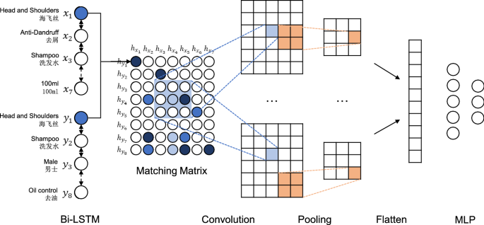

  

  The structure of TMM. TMM is designed for title matching. Bi-LSTM is used to represent each title as positional sentence representations, and generate an interaction matrix by interacting between those sentence representations. Then a CNN is used to extract features. These features are finally fed into a MLP to generate title similarity

• Convolution and pooling operation After obtaining the matching matrix, we apply typical convolutional neural network (CNN) to extract matching patterns. Assuming a kernel $z^k \in R^{r \times s}$, where k is the index of kernels, we scan over M from left to right and from top to bottom then output a future map $F_{i,j}^k$:

  $$\begin{aligned} F_{i,j}^k=\sum _{u=0}^{r-1}\sum _{v=0}^{s-1} z_{u,v}^k \cdot M_{i+u,j+v} +b^k, \end{aligned}$$

  (12)

  where i and j point to a certain position in the interaction matrix. Multiple feature maps are generated by different filters. Note that, the parameters are not shared among filters, thus they can capture different matching patterns. Then max-pooling operation is conducted to aggregate the most important information along each feature map:

  $$\begin{aligned} G^{k}_{i,j} = \max _{0 \le s< d_k}\max _{0 \le t < d'_k} F_{i \cdot d_k+s, j \cdot d'_k+t}^k, \end{aligned}$$

  (13)

  where $d_k$ and $d_k'$ denote the width and length of the corresponding pooling kernel.

• Title similarity Finally, we flatten the output of the pooling layer and concatenate them together as G. And we use a multi-layer perception (MLP) to produce title similarity $SIM_t$:

  $$\begin{aligned} SIM_t=\tanh (W \cdot G + b), \end{aligned}$$

  (14)

  where W and b are parameters and $\tanh (\cdot )$ is a nonlinear activation function.

It is worth noting that TMM is flexible in different applications. When only product titles are provided, TMM can be an independent model and title similarity is used as product matching score. On the contrary, when both product titles and attributes are provided, TMM can be used as a module and title similarity will be further combined with attributes similarity (introduced in Sect. 3.4) to generate the final product matching score.

Fig. 4

The structure of AMM. AMM is designed for attribute matching. The attribute names and values are processed separately. For attribute name matching, we use max pooling operation to extract the most similar pattern directly. For attribute value matching, we use 1-D convolution operation to extract matching patterns. The two matching features are fed into MLP and the MLP outputs the attribute similarity

3.4 AMM: attributes matching module

As the example showed in Fig. 1, the attributes are presented in name-value pairs. Product attribute names are analogous within a product category, and they are different across categories. In Fig. 1, product (a) and product (c) are two different products but they are both shampoos, thus they have some similar attribute names such as place of origin and N.W.. But attribute names are not always the same, like the attribute name “function” of product (a) has the similar meaning with the attribute name “effect” of product (b). Based on these observations, we compute the matching matrix based on word embedding to represent the similarity between the attribute names of two products. A max pooling operation is then conducted to extract the most important matching patterns. As for attribute values, things are different. For product (a) and product (c), they both have the attribute “N.W.”, but their attribute values are different, i.e. 750 ml and 730 ml. From that, we can distinguish these two products are different and mismatched because their size (N.W.) are different. Although “730 ml” and “750 ml” are close in the embedding space, they are different words essentially. These attribute values are pivotal for identifying whether products are identical and matched. Therefore, we cannot calculate the similarity between two sets of attribute values based on their embedding. Here we build attribute value matching matrix based on indicator function. And we design a special convolution operation to extract matching patterns. These features are further combined with attribute name matching features to generate attribute similarity. The matching structure of AMM is showed in Fig. 4.

Before we introduce the detail of AMM, we demonstrate the form of input data again. As the problem definition part we introduced in Sect. 3.1, both attribute names and values consist of several words. We segment the attribute names and values into two sets of words. For product X, the word set of attribute names is $(w_1^K, w_2^K, \ldots , w_u^K)$, while the word set of attribute values is $(w_1^V, w_2^V, \ldots , w_v^V)$. For Y, they are $(w'^K_1, w'^K_2, \ldots , w'^K_{u'})$ and $(w'^V_1, w'^V_2, \ldots , w'^V_{v'})$. Attribute name matching is conducted on word sets of attribute names in Sect. 3.4.1, and attribute value matching is processed on word sets of attribute values in Sect. 3.4.2.

3.4.1 Attribute name matching

We first build an interaction matrix between two word sets of attribute names. Like in the TMM, the similarity between two words is calculated by word embedding. The matrix measures the semantic similarities between two word sets of attribute names. In our example, the attribute name “function” would have a high similarity with the attribute name “effect”, and both of them represent similar meaning. After obtaining the matrix, we use K-Max pooling operation to extract top-k important matching patterns. Formally, the similarity $M^N_{i.j}$ between word of attribute name $w^K_i$ and $w'^K_j$ is computed as:

$$\begin{aligned} M^N_{ij} = e(w^K_i) \otimes e(w'^K_j), \end{aligned}$$

(15)

where e($\cdot$) represents the corresponding word embedding, and $\otimes$ is dot product here. Then the K-Max pooling operation is:

$$\begin{aligned} G^N = \max _k\{M^N\}, \end{aligned}$$

(16)

where $G^N$ is a vector with size $k \times 1$ that represents matching patterns of attribute names.

3.4.2 Attribute value matching

For attribute value matching, things are more complex. As we introduced, the similarity based on word embedding is not suitable here, since two different attribute values could be strong indicators for two products.

Here we use indicator function to build interaction matrix, i.e. for attribute value $w^V_i$ and $w'^V_j$, $M^V_{ij}$ is computed as:

$$\begin{aligned} M^V_{ij} = w^V_i \odot w'^V_j \end{aligned}$$

(17)

where $\odot$ is indicator function defined as:

$$\begin{aligned} a \odot b = {\left\{ \begin{array}{ll} 1 &{} {\text {if}}\,a\,\text {and}\,b\,{{\text {are}}\,{\text {the}}\,{\text {same}}\,{\text {words}}},\\ 0 &{} {\text {otherwise}}. \end{array}\right. } \end{aligned}$$

(18)

If calculating similarity of words by the indicator function, two different words in sets of attribute values cannot match, i.e. the similarity between “730 ml” and “750 ml” is 0.

Next, we use convolution operation to extract matching patterns. The size of convolution window is set as $v \times 1$ and the window moves horizontally. Our motivation is, for each attribute value word of product X, all identical words for product Y should be considered. To extract multiple matching patterns, we use L convolution kernels ($L=3$ in our example). After this step, L matching patterns are derived, and we flatten and concatenate them together as matching patterns of attribute values. Formally, the kth kernel $z'^k$ works on the matching matrix $M^V$ and outputs a matching pattern $F'^k$ where the ith element is computed as:

$$\begin{aligned} F'^k_i = \sum _{j=0}^{v'-1}z'^k_{j}\cdot M^V_{:,j} + b'^k. \end{aligned}$$

(19)

The size of $F'^k$ is $1 \times v'$. After being concatenated and flattened, we obtain attribute value matching patterns $G^V$ with size $(v' \times L) \times 1$.

3.4.3 Attribute similarity

After carrying out attribute name matching process and attribute value matching process, AMM generates two matching patterns. To mix the matching information of these two patterns, we concatenate them as a joint vector, which is a simple but effective method in practice (Zhang et al. 2015; Yan et al. 2016). The joint vector is then passed through a 2-layer MLP, which allows rich interactions between attribute names and attribute values. The features are extracted automatically and combined hierarchically from lower-level to higher-level. Finally, we obtain the attribute matching similarity $SIM_a$:

$$\begin{aligned} SIM_a = \tanh (W'\cdot [G^N:G^V] + b'), \end{aligned}$$

(20)

where $W'$ and $b'$ are parameters in MLP.

4 Two application scenarios

From the above sections, our model generates both the similarity between product titles ($SIM_t$) and the similarity between attributes ($SIM_a$). However, how to combine them depends on our different application scenarios:

4.1 A classification scenario

The first application scenario we simulated is on the consumers’ perspective: they select two products and want to compare them by their titles and attributes to judge whether they are identical and matched. In this scenario, the input is two product descriptions including their titles and attributes. The output is in two classes: 1—represents the two products are identical and 0—represents that they are different. Essentially, this is a classification problem. We concatenate $SIM_t$ and $SIM_a$ into a whole vector, and then feed it into a MLP to generate the probabilities on two classes. The class with higher probability is our predicted result.

We use the cross-entropy loss function to train our whole model:

$$\begin{aligned} L& {} = - \sum _{i=1}^{N}[y^{(i)}log(p_1^{(i)})+(1-y^{(i)})log(p_0^{(i)})], \end{aligned}$$

(21)

$$\begin{aligned} p_k& {} = \frac{e^{s_k}}{e^{s_0}+e^{s_1}},\quad k=0,1, \end{aligned}$$

(22)

where $y^{(i)}$ is the label of the ith data instance. $p_1^{(i)}$ is the predicted probability that the two inputs are identical products, while $p_0^{(i)}$ is on the contrary.

4.2 A ranking scenario

The second application scenario we considered is on the sellers’ or platform managers’ perspective: they use their own products as query products to retrieve similar products sold by other sellers or on other platforms. In this scenario, the input is a query product description and a list of candidate product descriptions. A product description consists of a product title and product attributes. The output is also a list of sorted candidate products. This is a ranking problem virtually. We concatenate $SIM_t$ and $SIM_a$ into a whole vector, then feed it into a MLP to generate a matching score for a given query product and a given candidate product. All candidate products are sorted by their matching scores to generate the result list.

Formally, given a triple ($q, d_+, d_-$), where q is the query product description, $d_+$ is the product that is identical with q, and $d_-$ is different with q. The goal of the ranking function is to rank $d_+$ higher than $d_-$. Thus the loss is:

$$\begin{aligned} L(q, d_+, d_-)=\max (0, 1-s(q,d_+) + s(q, d_-)), \end{aligned}$$

(23)

where $s(\cdot )$ denotes the matching scores output by our model.

5 Experiments

In this section, we conduct experiments to verify the effectiveness of our model and evaluate it in two scenarios we introduced. We first introduce the data set we use and various baselines, then introduce the evaluation metrics we used. The experimental results and analysis based on them are reported later.

5.1 Datasets

To build our data sets, we choose 20 product categories, including cosmetics, snacks, etc., to collect product description texts. We separately collect product data for each category from JD¹ and Tmall,² two most popular online platforms in China. There are more than hundreds of millions of products in JD and Tmall which cover varieties of categories. We finally crawl 695,171 products’ description texts from JD and crawl 382,907 products’ description texts from Tmall, and these data are used to train a Word2Vec (Mikolov et al. 2013b) model for obtaining word embedding. Each product’s description texts consist of a category type, a product title, several product attributes and a product brand name. Category type values are categories of products. Product titles are brief and free texts of products. Product attributes are provided in product detail pages by platforms to specify more details about products. The format of titles and attributes is different. Titles are short texts with semantic structure, while attributes are name-value pairs.

Matched and mismatched product pairs are used as positive and negative samples to train product matching models. To obtain these samples, we build a retrieval-based tagging system. This system uses an open source IR system (Solr³) to retrieve similar products in Tmall when given a product title in JD as query. In the process of manual labeling, we choose a lot of popular products in different categories from JD, and utilize the tagging system to retrieve similar products from Tmall for each selected popular product. Then we label these product pairs with matched and mismatched labels. Finally, these matched pairs and mismatched pairs are stored in database. The criterion for determining whether two products are matched is the consistence of their product brands and key product specifications. This annotation needs much human resource, thus we eventually label 30,545 matched product pairs. Each pair consists of a product from JD and a product from Tmall. For the generation of mismatched pairs, we use our tagging system to retrieve similar but mismatched products for each query product instead of using random sampling, which is mainly because we expect our model to be able to distinguish similar products and this is also consistent with real application scenarios. To guarantee the correctness of labeling, we invite several experienced e-commercial platform workers for manual labeling and inspection.

The statistic of the data set is showed in Table 1. We divide the data set of matched pairs based on product categories, and split them into positive pairs of training set and test set with a ratio of 4:1. For each positive pair in data set, we use the aforementioned sampling strategy to generate some mismatched pairs (regarded as negative pairs) and add them into corresponding data set. Specifically, for each product title, we retrieve 100 negative products by our tagging system. All of them are used in our ranking scenario. As for the classification scenario, 10 of them were selected randomly as negative products, and we adopt over-sampling method to ensure the equilibrium of categorical data. We use fivefold cross validation to get validation set from training data to tune the parameters of our model.

Table 1 The statistic of data set

5.2 Experimental settings

Our model is implemented based on TensorFlow.⁴ The optimization of our model is conducted with Adam optimizer (Kingma and Ba 2014). For network configurations (e.g., the size of word embedding and hidden layer sizes), we set the batch size as 64 and tune these hyper-parameters based on our validation set. Word embedding is initialized by Word2Vec. The embedding size is tested in 50, 100, 200. The learning rate is selected from 1e$-$3, 1e$-$4, 1e$-$5. In the network architecture of TMM, we select 20 as the maximum length of product titles. Titles with more than 20 words are truncated and ones with less than 20 words are padded by zero vectors. And we select the hidden layer size of Bi-LSTM from 50, 100, 200. Convolution window size and pooling window size are from ${2 \times 2, 3 \times 3, 4 \times 4}$. In network architecture of AMM, we select k value of K-Max pooling layer from 10, 20, 30 and the kernel number in attribute value matching layer from 50, 100, 200.

Final optimal hyper-parameters are determined by grid search in validation set. Early stopping is used to prevent over fitting. Finally, we set the word embedding size as 100, and set learning rate as 1e$-$3. In TMM, we use 100 as hidden layer size, and select $2 \times 2$ as convolution window size and pooling window size. In AMM, we use 20 as k value 50 as kernel numbers. Following Zamani et al. (2018), we use tanh as the activation function for all hidden layer.

5.3 Evaluation metrics

Since our experiments are conducted in two application scenarios, the evaluation metrics are different.

In the classification scenario, we use Precision, Recall and F1 to evaluate the models. Precisely, assume the number of matched pairs is T (true samples) and the number of mismatched pairs is F (false samples). The number of pairs predicted as matched by the model is P, while the number of samples predicted as mismatched is N. Under this circumstance, Precision, Recall and F1 are defined as follows:

$$\begin{aligned} \text {Precision}& {} = {TP}/{(TP+FP)}, \\ \text {Recall}& {} = {TP}/{P}, \\ \text {F1}& {} = {2}/({1/\text {Precision}+1/\text {Recall}), } \end{aligned}$$

where TP denotes the number of pairs which are matched and also correctly predicted as matched by the model. FP is the number of pairs that are mismatched but wrongly predicted as matched by the model.

In the ranking scenario, we use the precision at 1 (P@1 shortly), mean reciprocal rank (MRR shortly) and mean average precision (MAP shortly).

P@1 calculates mean precision of top one product for all ranking lists. MRR measures average position of first matched product for all ranking lists. We have:

$$\begin{aligned} \text {P@1}& {} = \frac{1}{N}\sum _{i=1}^{N}{\delta ({rank(S_Y^{+(i)})=1}}) , \\ \text {MRR}& {} = \frac{1}{N}\sum _{i=1}^{N}\left( \frac{1}{rank(S_Y^{+(i)})}\right) , \end{aligned}$$

where N is the number of ranking lists in test set. $S_Y^{+(i)}$ is the first matched product in the ith ranking list, $rank(\cdot )$ denotes the rank of a item in the ranking list, and $\delta$ is the indicator function.

MAP is mean of average precision scores for all ranking lists. This metric is computed as follows:

$$\begin{aligned} \text {AveP(i)}& {} = \frac{1}{R^{(i)}}\sum _{r=1}^{R^{(i)}} \frac{r}{rank(S_Y^{r+(i)})},\\ \text {MAP}& {} = \frac{1}{N}\sum _{i=1}^{N}AveP(i), \end{aligned}$$

where AveP(i) denotes average precision score of the ith ranking list, $R^{(i)}$ is the number of matched products in the ith ranking list. $S_Y^{r+(i)}$ denotes the rth matched item in the ith ranking list.

5.4 Baseline models

We apply a product retrieval approach to product matching problem based on product attributes.

• PM-LM (Duan et al. 2013): PM-LM is a probabilistic entity retrieval model based on query generation. The model is proposed to optimize search over structured product entities with keyword queries. When extending this method to product matching problem, we use the product title from JD as query to retrieve structured product attributes from Tmall. The ranking process is based on the likelihood that product attributes are matched with the given product title. This entity retrieval model can only be applied to our ranking scenario.

Many text matching models have been proposed, thus we compare our model with some state-of-the-art text matching models. We firstly apply these text matching models for product matching by considering only product titles. And we trivially extend these models to work with title and attributes by concatenating all of them into a single text instance. We use t as the subscript to indicate that the matching model only considers product titles to match, and use ta to denote that the model considers both titles and attributes.

• ARC-I (Hu et al. 2014): ARC-I uses layers of convolution and pooling to generate the fixed length compositional representation for each text, and then merges them as the input of the last layer to generate final matching score.

• ARC-II (Hu et al. 2014): ARC-II first builds interaction spaces between two texts by 1D convolution, and conducts interaction operation to consider the similarities between any two segments from two texts instead of considering the similarities between any words from two texts. Then layers of 2D convolution and pooling are used to obtain high level features. Finally, MLP is used to generate matching score.

• MatchPyramid(CNN) (Pang et al. 2016): MatchPyramid firstly interacts between two texts to generate the matching matrix, then uses hierarchical convolution and pooling to capture rich matching patterns, finally adopts MLP as the final layer to generate the matching score or classification result.

• MV-LSTM(Bi-LSTM + K-Max pooling) (Wan et al. 2016): MV-LSTM firstly adopts bi-directional long short term memory (Bi-LSTM) to generate multiple positional sentence representations for each sentence, and then interacts between these positional sentence representations to form interaction matrix by using different similarity functions. Finally adopts K-Max pooling strategy to select important features as the input of the multi-layer perceptron (MLP).

• KNRM (Xiong et al. 2017): KNRM is a kernel based neural model for document ranking. It uses word embedding to measure word-level similarity and generates a translation matrix. Then it adopts kernel-pooling technique to extract multi-level soft matching features from translation matrix, finally these features are used as the input of learning-to-rank layer to get final ranking score. The training process is end-to-end and pair-wise ranking loss function is used to implement document ranking.

• DRMM (Guo et al. 2016): DRMM first builds local interaction between each pair of words from queries and documents, then transforms the variable-length local interaction matrix into fixed-length matching histogram to obtain matching degree for each word in queries, finally it generates final ranking scores based the weighted sum of matching degrees and word weights that obtained by word embedding or TF-IDF.

• DUET (Mitra et al. 2017): DUET is a document ranking model that consists of distributed model and local model, and it matches texts by considering both distributed representations and traditional local representations. The local model uses one-hot encoding to represent words and emphasizes exact matching while distributed model uses distributed embedding to represent words and concerns semantic matching. Then the sum of two scores generated from the two models is final ranking score and the two models are jointly trained as part of a single neural network.

It is worth noting that we use Bi-LSTM to generate positional representations for each title in our title matching module (TMM). Meanwhile, we also replace Bi-LSTM with a single direction LSTM and compare them:

• LSTM + CNN: We adopt long short term memory (LSTM) to generate multiple representations for each sentence, and use these representations to generate interaction matrix, then CNN is used to select features. Finally, these features are feed into a MLP. The only difference between itself and our title matching module is the difference between LSTM and Bi-LSTM. Experimental purpose of LSTM + CNN is to make a contrast with TMM and verify the usefulness of Bi-LSTM.

We also extend an information retrieval model to work with product titles and attributes by regarding products as documents with multiple fields.

• NRM-F (Zamani et al. 2018): NRM-F is a document ranking model that takes advantage of full document structure. The model matches each query with multiple fields that consists of multiple instances. We apply this model to our product matching problem by regarding two input products as two documents with multiple fields. The model semantically represents two products separately. For the semantic representation of products, NRM-F first uses convolution layers and pooling layers to obtain instance-level representations, then aggregates these instance-level representations to generate field-level representations. Finally, all field-level representations are concatenated to generate product representations. After getting two product representations, the model uses Hadamard product to compare across all the field representations and obtain their final interaction similarities. These similarities are finally fed into a MLP to obtain a final matching score.

Since two modules in our model (TMM and AMM) can also work separately, we also conduct experiments on them respectively.

5.5 Experimental results and analysis

To evaluate the performance of these product matching models, we apply these models to a ranking scenario and a classification scenario and evaluate these models based on their respective evaluation metrics. We show the experimental results in Table 2.

Table 2 Experimental results of PMM model and other baselines

Table 3 Experimental results of TMM model based different interaction methods

We compare the performance of baseline models with our proposed title matching module (TMM), attribute matching module (AMM) and product matching model (PMM). Two-tailed paired Student’s t test is performed to compare our product matching model (PMM) with all baselines. And no adjustment is conducted on the t test. Values showing significant improvement over baseline methods are marked ($\ddagger$ for p value < 0.01 and $\dagger$ for p value < 0.1).

In our title matching module (TMM), bidirectional long-term and short-term memory neural networks are used to semantically represent product titles, and different methods can be introduced to interact between titles. Experimental results of TMM by using different interaction methods are showed in Table 3. From the table, we can see that Cosine interaction method ($TMM_{cosine}$) outperforms other interaction methods, including $TMM_{euclidean}$, $TMM_{dot}$ and $TMM_{Bilinear}$. And Student’s t test is conducted to compare $TMM_{cosine}$ with other interaction methods. Results show very significant improvement (p value < 0.01) over $TMM_{Bilinear}$ and $TMM_{dot}$ , and show significant improvement (p value < 0.05) over $TMM_{euclidean}$.

From experimental results in Table 2, we see that our title matching module $TMM_{cosine}$ outperforms all selected text matching baselines, including $ARC-I_t$, $ARC-II_t$, $MatchPyramid_t$, $MV-LSTM_t$, $DRMM_t$, $KNRM_t$, and $DUET_t$, which shows the combination of RNNs and CNNs in our model is a better way to exact product matching features. We also observe that $TMM_{cosine}$ outperforms $LSTM+CNN_t$. This explains that Bi-LSTM can better represent product titles than LSTM. Compared with TMM and AMM, PMM has a better experimental performance, which is expected because PMM leverages both product titles and attributes and it models product titles and product attributes separately. All these also indicate the feasibility and usefulness of our model structure.

The experimental performance of AMM is slightly worse than some other models. We observe our data set and discover that many important product specifications are incomplete or missing in attributes. Based on the reason, the performance of AMM is not considerable, thus combining product attributes as supplementary information with product titles is more reasonable.

We compare text matching models that use product titles to match with those that consider both product titles and attributes to match, experimental results show that there is little improvement or even a decline, which is mainly because the formats of titles and attributes are different, and concatenating them directly is inappropriate. PMM considers the different format of titles and attributes, and it uses different modules to extract their different matching features. We compare it with NRM-F that also considers products’ structure and text matching models that concatenating title and attributes directly to match. Results show that PMM and NRM-F outperform these text matching models, which illustrates that considering the different formats of titles and attributes is beneficial for product matching.

PM-LM is an unsupervised entity retrieval model, and we extend it as a product matching model in our ranking scenario. It outperforms our many neural text matching baselines, and shows that the product language model can well describe structured product attributes, and structured attributes are generally conducive to product matching.

5.6 Model extension

In this section, we first investigate some classic machine learning models in general classification and ranking problems. Then we extract some handcraft features to verify if our model can be further improved.

5.6.1 Classic machine learning models

For the first attempt, note that both title matching result and attribute matching result generated by TMM and AMM are vectors (features), thus it is easy to apply other machine learning methods based on them. To achieve this, we remove MLP in our PMM and train TMM and AMM separately to obtain the title matching features and attribute matching features. Then we feed these features into SVM, Naive Bayes and Decision tree for classification scenario, and feed them into Mart and LambdaMart for ranking scenario. We denote these models as:

• TMM + AMM + SVM: we adopt SVM to train classification model by considering the outputs of both TMM and AMM.

• TMM + AMM + Bayes: we adopt Bayes to train classification model by considering the outputs of both TMM and AMM.

• TMM + AMM + Decision tree: we adopt Decision tree to train classification model by considering the outputs of both TMM and AMM.

• TMM + AMM + Mart: we adopt Mart to train ranking model by considering the outputs of both TMM and AMM.

• TMM + AMM + LambdaMart: we adopt LambdaMart to train ranking model by considering the outputs of both TMM and AMM.

5.6.2 Handcraft features

In order to verify if our model can be further augmented, we extract some handcraft features:

• The number and proportion of co-occurrence words and characters of two products titles;

• The number of co-occurrence digits and letters in the titles and attribute values of two products;

• The Jaccard similarity between titles, attribute names and attribute values of two products;

• The similarity between TF-IDF vectors of two product titles.

Then we add these features into aforementioned advanced models, and we denote them as:

• TMM + AMM + extra features + SVM: Different from TMM + AMM + SVM, we also consider extra features to train classification model.

• TMM + AMM + extra features + Bayes:Different from TMM + AMM + Bayes, we also consider extra features to train classification model.

• TMM + AMM + extra features + Decision tree: Different from Decision tree, we also consider extra features to train classification model.

• TMM + AMM + extra features + Mart: Different from TMM + AMM + Mart, we also consider extra features to train ranking model.

• TMM + AMM + extra features + LambdaMart: Different from TMM + AMM + LambdaMart, we also consider extra features to train ranking model.

Table 4 Experimental results under classification scenario

Table 5 Experimental results under ranking scenario

For each machine learning classification algorithm, we train two models separately by considering whether extra features are added to training stage. The experimental results are showed in Table 4. We compare machine learning classification models with PMM, and we find that PMM works best. The potential reason is that both TMM and AMM are trained simultaneously in PMM, which leads to better performance than other models. By comparisons, we also observe that the performance of Naive Bayes is slightly better than SVM and Decision Tree. Besides, for each classification algorithm, we compare the performance of the model that considering extra features and the model that not considering these features to judge the usefulness of extra features. And we find that there is little improvement and the usefulness of extra features is not obvious under classification scenario.

For each ranking algorithm, we also train two ranking models separately by considering whether extra features are added to training stage. The experimental results are showed in Table 5. We compare these learning to rank algorithms with PMM, and we find PMM works best, which is consistent with classification scenario. And the performance of LambdaMart is better than MART, which is in line with expectation. Whether for LambdaMart or for Mart, we consider the outputs of both TMM and AMM to train ranking models, and also consider adding extra features to train ranking models. After comparisons, we find that the improvement of ranking models considering extra features is not great, which also explain that the features extracted automatically from our neural product matching model are effective.

6 Conclusion

In order to study the problem of identifying identical products on different platforms, we proposed a neural product matching model by considering the respective characteristics of product titles and attributes, and we casted the problem as ranking and classification scenarios. We also tried different classical classification algorithms and ranking algorithms to combine our neural matching features and some other features. The experiments were conducted on the data collected from real online platforms and the results showed that our model can outperform all the state-of-the-art models under both classification and ranking scenarios. In the future, we will further explore a better way to measure the importance of different attributes, and take into account more product information (such as product pictures and richer product descriptions) for product matching.

References

Christen, P. (2012). Data matching: Concepts and techniques for record linkage, entity resolution, and duplicate detection. Data-Centric Systems and Applications, Springer 2012 (pp. 1–270).
Duan, H., & Zhai, C. X. (2015). Mining coordinated intent representation for entity search and recommendation. In Proceedings of the 24th ACM international conference on information and knowledge management, CIKM 2015, Melbourne, VIC, Australia, October 19–23, 2015 (pp. 333–342).
Duan, H., Zhai, C. X., Cheng, J., & Gattani, A. (2013). Supporting keyword search in product database: A probabilistic approach. PVLDB, 6(14), 1786–1797.
Fellegi, I. P., & Sunter, A. B. (1969). A theory for record linkage. Publications of the American Statistical Association, 64(328), 1183–1210.
Gopalakrishnan, V., Sengamedu, S., Sengamedu, S., Sengamedu, S., & Sengamedu, S. (2012). Matching product titles using web-based enrichment. In ACM international conference on information and knowledge management (pp. 605–614).
Guo, J., Fan, Y., Ai, Q., & Croft, W. B. (2016). A deep relevance matching model for ad-hoc retrieval. In Proceedings of the 25th ACM international conference on information and knowledge management, CIKM 2016, Indianapolis, IN, USA, October 24–28, 2016 (pp. 55–64).
Hu, B., Lu, Z., Li, H., & Chen, Q. (2014). Convolutional neural network architectures for matching natural language sentences. In Advances in neural information processing systems 27: Annual conference on neural information processing systems 2014, December 8–13 2014, Montreal, Quebec, Canada (pp. 2042–2050).
Huang, P.-S., He, X., Gao, J., Deng, L., Acero, A., & Heck, L. P. (2013). Learning deep structured semantic models for web search using clickthrough data. In 22nd ACM international conference on information and knowledge management, CIKM’13, San Francisco, CA, USA, October 27–November 1, 2013 (pp. 2333–2338).
Kannan, Anitha, Givoni, I. E., Agrawal, R., & Fuxman, A. (2011). Matching unstructured product offers to structured product specifications. In Proceedings of the 17th ACM SIGKDD international conference on knowledge discovery and data mining, San Diego, CA, USA, August 21–24, 2011 (pp. 404–412).
Kingma, D. P., & Ba, J. (2014). Adam: A method for stochastic optimization. CoRR arXiv:1412.6980.
Köpcke, H., Thor, A., Thomas, S., & Rahm, E. (2012). Tailoring entity resolution for matching product offers. In 15th international conference on extending database technology, EDBT ’12, Berlin, Germany, March 27–30, 2012, proceedings (pp. 545–550).
Mikolov, T., Chen, K., Corrado, G., & Dean, J. (2013a). Efficient estimation of word representations in vector space. CoRR, arXiv:1301.3781.
Mikolov, T., Sutskever, I., Chen, K., Corrado, G. S., & Dean, J. (2013b). Distributed representations of words and phrases and their compositionality. In Advances in neural information processing systems 26: 27th annual conference on neural information processing systems 2013. Proceedings of a meeting held December 5–8, 2013, Lake Tahoe, Nevada, United States (pp. 3111–3119).
Mitra, B., & Craswell, N. (2018). An introduction to neural information retrieval. Foundations and Trends in Information Retrieval, 13(1), 1–126.
Mitra, B., Diaz, F., & Craswell, N. (2017). Learning to match using local and distributed representations of text for web search. In Proceedings of the 26th international conference on World Wide Web, WWW 2017, Perth, Australia, April 3–7, 2017 (pp. 1291–1299).
Nauman, F., & Herschel, M. (2010). An introduction to duplicate detection. Synthesis Lectures on Data Management, 2(1), 1–87.
Onal, K. D., Zhang, Y., Altingovde, I. S., Rahman, Md., Mustafizur, K., Pinar, B., et al. (2018). Neural information retrieval: At the end of the early years. Information Retrieval Journal, 21(2–3), 111–182.
Pang, L., Lan, Y., Guo, J., Xu, J., Wan, S., & Cheng, X. (2016). Text matching as image recognition. In Proceedings of the thirtieth AAAI conference on artificial intelligence, February 12–17, 2016, Phoenix, Arizona, USA (pp. 2793–2799).
Qiu, X., & Huang, X. (2015). Convolutional neural tensor network architecture for community-based question answering. In Proceedings of the twenty-fourth international joint conference on artificial intelligence, IJCAI 2015, Buenos Aires, Argentina, July 25–31, 2015 (pp. 1305–1311).
Schuster, M., & Paliwal, K. K. (1997). Bidirectional recurrent neural networks. IEEE Transaction on Signal Processing, 45(11), 2673–2681.
Shen, Y., He, X., Gao, J., Deng, L., & Mesnil, G. (2014). Learning semantic representations using convolutional neural networks for web search. In 23rd international World Wide Web conference, WWW ’14, Seoul, Republic of Korea, April 7–11, 2014, Companion Volume (pp. 373–374).
Van Gysel, C., de Rijke, M., & Kanoulas, E. (2016). Learning latent vector spaces for product search. In Proceedings of the 25th ACM international conference on information and knowledge management, CIKM 2016, Indianapolis, IN, USA, October 24–28, 2016 (pp. 165–174).
Wan, S., Lan, Y., Guo, J., Xu, J., Pang, L., & Cheng, X. (2016). A deep architecture for semantic matching with multiple positional sentence representations. In Proceedings of the thirtieth AAAI conference on artificial intelligence, February 12–17, 2016, Phoenix, Arizona, USA (pp. 2835–2841).
Winkler, W. (2006). Overview of record linkage and current research directions (pp. 603–623). Suitland: Bureau of the Census.
Winkler, W. E. (1999). The state of record linkage and current research problems. Suitland: Statistical Research Division, U.S. Census Bureau.
Xiong, C., Dai, Z., Callan, J., Liu, Z., & Power, R. (2017). End-to-end neural ad-hoc ranking with kernel pooling. In Proceedings of the 40th international ACM SIGIR conference on research and development in information retrieval, Shinjuku, Tokyo, Japan, August 7–11, 2017 (pp. 55–64).
Yan, R., Wu, H., Wu, H., & Wu, H. (2016). “Shall I be your chat companion?”: Towards an online human–computer conversation system. In ACM international on conference on information and knowledge management (pp. 649–658).
Zamani, H., Mitra, B., Song, X., Craswell, N., & Tiwary, S. (2018). Neural ranking models with multiple document fields. In Proceedings of the Eleventh ACM international conference on web search and data mining, WSDM 2018, Marina Del Rey, CA, USA, February 5–9, 2018 (pp. 700–708).
Zhang, B., Su, J., Xiong, D., Lu, Y., Duan, H., & Yao, J. (2015). Shallow convolutional neural network for implicit discourse relation recognition. In Conference on empirical methods in natural language processing (pp. 2230–2235).
Acknowledgements
This work was supported by National Key R&D Program of China No. 2018YFC0830703, National Natural Science Foundation of China No. 61872370, and the Fundamental Research Funds for the Central Universities, and the Research Funds of Renmin University of China No. 2112018391.
Author information
Authors and Affiliations
Corresponding author
Additional information
Publisher's Note
Springer Nature remains neutral with regard to jurisdictional claims in published maps and institutional affiliations.
Rights and permissions
About this article
Cite this article
Li, J., Dou, Z., Zhu, Y. et al. Deep cross-platform product matching in e-commerce. Inf Retrieval J 23, 136–158 (2020). https://doi.org/10.1007/s10791-019-09360-1
Received:
Accepted:
Published:
Issue Date:
DOI: https://doi.org/10.1007/s10791-019-09360-1