

Abstract
Ambiguous visual images can generate dynamic and stochastic switches in perceptual interpretation known as perceptual rivalry. Such dynamics have primarily been studied in the context of rivalry between two percepts, but there is growing interest in the neural mechanisms that drive rivalry between more than two percepts. In recent experiments, we showed that split images presented to each eye lead to subjects perceiving four stochastically alternating percepts (Jacot-Guillarmod et al. Vision research, 133, 37–46, 2017): two single eye images and two interocularly grouped images. Here we propose a hierarchical neural network model that exhibits dynamics consistent with our experimental observations. The model consists of two levels, with the first representing monocular activity, and the second representing activity in higher visual areas. The model produces stochastically switching solutions, whose dependence on task parameters is consistent with four generalized Levelt Propositions, and with experiments. Moreover, dynamics restricted to invariant subspaces of the model demonstrate simpler forms of bistable rivalry. Thus, our hierarchical model generalizes past, validated models of binocular rivalry. This neuromechanistic model also allows us to probe the roles of interactions between populations at the network level. Generalized Levelt’s Propositions hold as long as feedback from the higher to lower visual areas is weak, and the adaptation and mutual inhibition at the higher level is not too strong. Our results suggest constraints on the architecture of the visual system and show that complex visual stimuli can be used in perceptual rivalry experiments to develop more detailed mechanistic models of perceptual processing.
Keywords: Binocular rivalry, Interocular grouping, Levelt’s propositions, Hierarchical model
1. Introduction
When conflicting images are presented to different eyes, our visual system often fails to produce a stable fused percept. Instead, perception stochastically alternates between the presented images (Wheatstone 1838; Levelt 1965; Leopold and Logothetis 1999; Blake and Logothetis 2002; Blake 2001; Bressler et al. 2013). More generally, multistable binocular rivalry between more than two percepts can occur when images presented to each eye can be partitioned and regrouped into coherent percepts. For example, subjects presented with the jumbled images in Fig. 1a may alternatively perceive a monkey face, or the jungle scene shown in Fig. 1b (Kovacs et al. 1996). In these cases perception evolves dynamically under constant stimuli, revealing aspects of the cortical mechanisms underlying visual awareness (Leopold and Logothetis 1999; Tong et al. 2006; Sterzer et al. 2009; Leopold and Logothetis 1996; Polonsky et al. 2000).
Fig. 1.
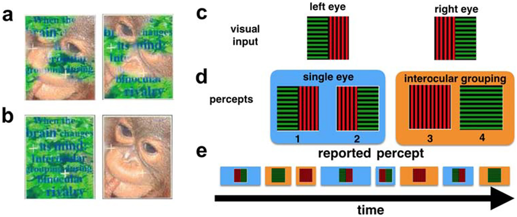
Multistable perceptual rivalry. The fragmented images presented to the left and right eyes in a can lead to the coherent percepts shown in b Kovacs et al. (1996). c An example of the stimuli presented to the left and right eyes in Jacot-Guillarmod et al. (2017). Gratings were always split so that halves with the same color and orientation could be matched via interocular grouping, but were otherwise randomized across trials and blocks (See Jacot-Guillarmod et al. (2017) for experimental methods). d Subjects typically reported seeing one of four percepts – two single-eye and two grouped – at any given time during a trial. e A typical perceptual time series reported by a subject, showing the stochasticity in both the dominance times and the order of transitions between percepts
While the literature on bistable binocular rivalry is extensive, far fewer studies have addressed multistable percepts. Rivalry between multiple percepts likely involves higher level image recognition, as well as monocular competition (Kovacs et al. 1996; Suzuki and Grabowecky 2002; Huguet et al. 2014; Golubitsky et al. 2019), suggesting a noninvasive way to probe perceptual mechanisms across cortical areas, and offering a broader picture of visual processing.
Here, we build on previous models to provide a mechanistic account of perceptual multistability due to interocular grouping effects (Laing and Chow 2002; Wilson 2003; Moreno-Bote et al. 2007; Shpiro et al. 2007; Said and Heeger 2013; Dayan 1998). We propose a mechanism that involves different levels of visual cortical processing by building a hierarchical neural network model of binocular rivalry with interocular grouping. Our model captures the qualitative dynamics of perceptual switches reported by human subjects in experiments described by (Jacot-Guillarmod et al. 2017) involving the visual stimuli shown in Fig. 1c. When presented with these stimuli, subjects reported alternations between four percepts, two single-eye percepts, and two grouped percepts that combined two halves of each stimulus into a coherent whole (See Fig. 1d).
Levelt’s four propositions (1965) capture the hallmarks of bistable binocular rivalry by relating stimulus strength (such as contrast or luminance), dominance duration (the time interval during which a single percept is reported), and predominance (the fraction of the time a percept is reported). Jacot-Guillarmod et al. (2017) have provided experimental support for a generalized version of Levelt’s propositions, and our model suggests neural mechanisms that drive the underlying cortical dynamics encoding perceptual changes.
Levelt’s propositions describe well–tested statistical properties of perceptual alternations (Laing and Chow 2002; Brascamp et al. 2006; Wilson 2007; Moreno-Bote et al. 2010; Klink et al. 2010; Seely and Chow 2011), and provide constraints on mechanistic models of binocular rivalry. Successful models broadly explain rivalry in terms of three interacting neural mechanisms: Mutual inhibition drives the exclusivity of the perceived patterns; Slow adaptation drives the transition between the different percepts; Finally, internally generated noise is necessary to account for the observed variability in perceptual switching times (Matsuoka 1984; Lehky 1988; Arrington 1993; Lumer 1998; Kalarickal and Marshall 2000; Laing and Chow 2002; Lago-Fernandez and Deco 2002; Stollenwerk and Bode 2003; Wilson 2003; Noest et al. 2007; Seely and Chow 2011; Freeman 2005; Brascamp et al. 2006; Moreno-Bote et al. 2007).
In our model we include these mechanisms, along with additional, abstracted features of the visual system. The model contains a lower level associated with early (e.g., eye-based) neural processes and tuned to geometric stimulus properties (e.g. orientation), and a higher level which accounts for complex pattern grouping and is responsible for the formation of late stage percepts. Our model thus extends earlier models of bistable binocular rivalry, and it reduces to simpler rivalry models under bistable inputs (Wilson 2003; Tong et al. 2006; Diekman et al. 2013).
We hypothesize that pattern grouping effects occur already at the early stages of the visual system. We thus assume that the connectivity of the first layer in our network is modulated by cues – in our case color saturation – indicating which parts of the percepts belong to the same group. In most previous models of rivalry the strength of the stimulus primarily modulated the inputs to various network modules. In our case, we assume that the input strength (i.e., color saturation of the oriented grid) changes the connectivity between the neuronal populations encoding the two halves of images of the same color and orientation, consistent with the experimental results of Ramachandran et al. (1973) and Kim and Blake (2007), which indicate that color promotes interocular grouping.
We found that over a range of parameters the model also displays dynamics consistent with the generalized version of Levelt’s Propositions proposed by Jacot-Guillarmod et al. (2017). Our results hold under weak feedback from the higher to the lower level. However, we observed these dynamics only with strong mutual inhibition between populations representing conflicting stimuli at the lower level of the visual hierarchy. Our model thus suggests constraints on the interactions between neural populations in the visual system.
Our study thus shows that more complex visual stimuli can be used in perceptual rivalry experiments to drive the development of more detailed mechanistic models of perceptual processing (Wilson 2003; Dayan 1998; Freeman 2005).
2. Methods
2.1. Hierarchical model of perceptual multistability with interocular grouping
Considerable evidence suggests that visual processing in humans and other mammals is organized hierarchically (Polonsky et al. 2000; Tong 2001; Leopold and Logothetis 1996; Logothetis and Schall 1989; Sheinberg and Logothetis 1997; Dayan 1998; Wilson 2003; Freeman 2005; Tong et al. 2006). The simplest models of such processing assume that visual areas at the higher level of the hierarchy pool the activity of lower areas (Riesenhuber and Poggio 1999). Here we extend previous, non-hierarchical models of perceptual rivalry (Laing and Chow 2002; Wilson 2009; Moreno-Bote et al. 2007; Huguet et al. 2014; Diekman et al. 2013) to a model that spans two levels of the visual hierarchy, and study grouping in perceptual competition. A schematic representation of our model is shown in Fig. 2. The sub-network at the first level of the hierarchy consists of four neural populations, each receiving input from a different hemifield of the two eyes (See also Fig. 6C of Diekman et al. (2013) and Fig. 2B of Tong et al. (2006)). The responses of all four possible pairs of populations at the first level are integrated by distinct populations at the second level (Laing and Chow 2002; Wilson 2003; Moreno-Bote et al. 2007). Each of the four populations at the second level corresponds to one of the four percepts shown in Fig. 1b.
Fig. 2.
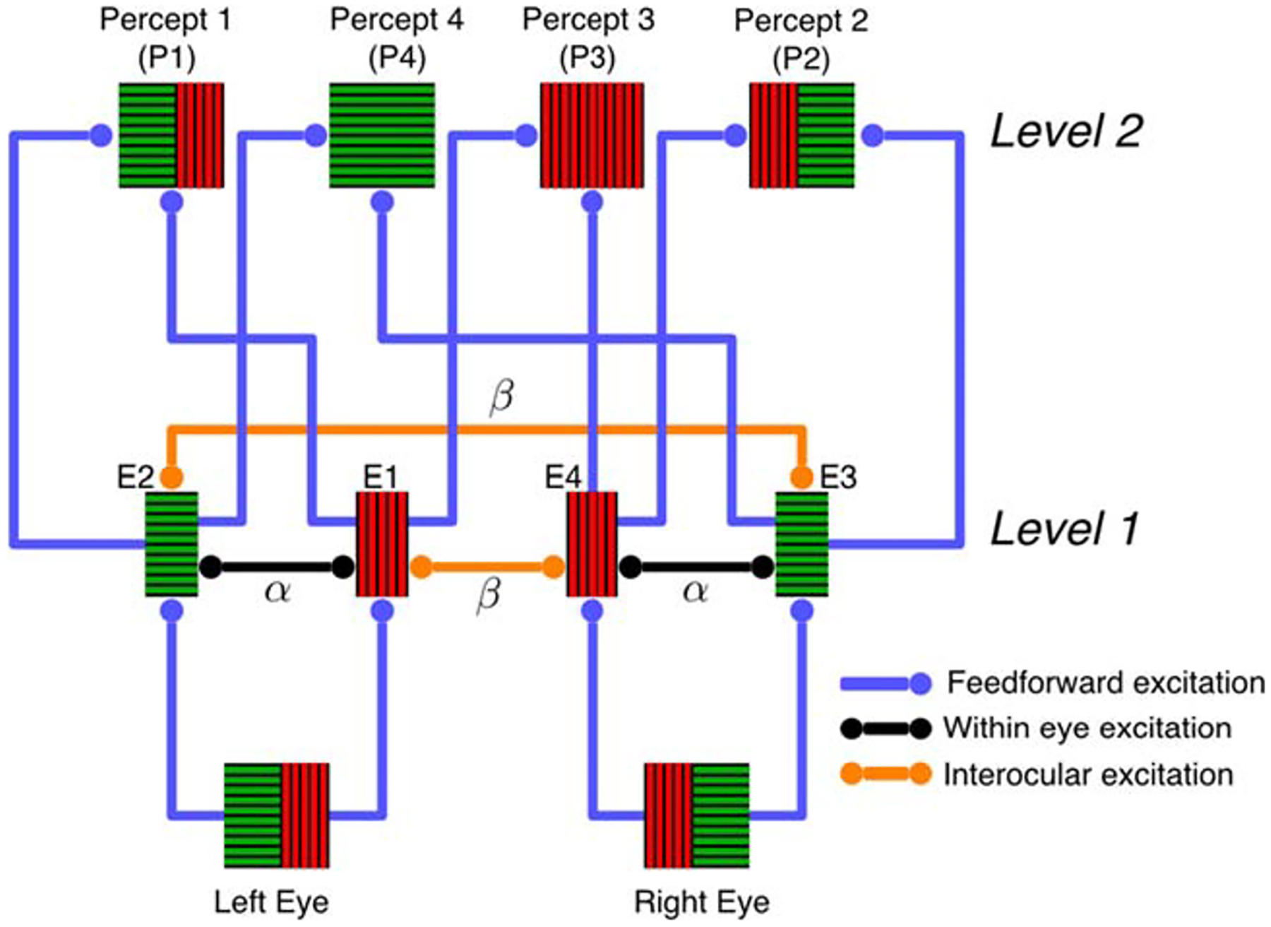
A hierarchical model of interocular grouping. Neural populations representing stimuli to the four hemifield-eye combinations at Level 1 provide feedforward input to populations representing integrated percepts at Level 2, as described by Eqs. (1) and (4) (See also Fig. 6C of Diekman et al. (2013) and Fig. 2B of Tong et al. (2006)). The figure shows recurrent excitation within Level 1. To avoid clutter, mutual inhibition between the same hemifield of opposite eyes is not shown. All populations at the second level of the hierarchy mutually inhibit one another (Laing and Chow 2002; Wilson 2003; Moreno-Bote et al. 2007)
A key feature of our model is the presence of excitatory coupling between populations receiving input from different hemifields both from the same and from different eyes. This is consistent with electrophysiology and tracing experiments that reveal long-range horizontal connections between neurons in area V1 with non-overlapping receptive fields, but similar orientation preferences (Stettler et al. 2002; Sincich and Horton 2005). We also assumed inhibitory coupling between populations receiving conflicting input from the same hemifield of different eyes, e.g. the left hemifield of the left and the left hemifield of the right eye. Experimental literature suggests cells with orthogonal orientation preferences can inhibit one another through multisynaptic pathways involving recurrent and feedback circuitry (Ringach et al. 1997; Ferster and Miller 2000). Finally, we assumed that all populations at the second level inhibit each other, as in previous computational models (Laing and Chow 2002; Moreno-Bote et al. 2007; Shpiro et al. 2007; Lankheet 2006; Seely and Chow 2011).
The two levels thus form a processing hierarchy (Wilson 2003; Tong et al. 2006) with the first roughly associated with monocular neural activity generated in LGN and V1 (Wilson 2003; Blake 1989; Polonsky et al. 2000; Tong 2001), and the second level associated with the activity of higher visual areas, such as V4 and MT, that process objects and patterns (Leopold and Logothetis 1999; Wilson 2003; Lamme and Roelfsema 2000). However, each level could also describe multiple functional layers of the visual system (Sterzer et al. 2009).
First level of the visual hierarchy
The activity of each neural population receiving input from one of the four hemifield-eye combinations at Level 1 is described by a firing rate variable Ei, i = 1, 2, 3, 4 (corresponding to left hemi/left eye; right hemi/left eye; left hemi/right eye; and right hemi/right eye, see Fig. 2). To model adaptation, we included variables describing hyperpolarizing currents activated at elevated firing rates, Hi, with i = 1, 2, 3, 4 (Benda and Herz 2003). The firing rates at the lower level of the visual hierarchy are then governed by the following equations:
| (1a) |
| (1b) |
| (1c) |
| (1d) |
| (1e) |
| (1f) |
| (1g) |
| (1h) |
with activity time constant τ = 10ms, and adaptation time constant τh = 1000ms (Häusser and Roth 1997). The inputs, Ii, model the strength of the stimulus in each hemifield, and g is the strength of adaptation. We assumed that all inputs, Ii, all are equal in intensity, so that Ii = I for i = 1, 2, 3, 4. This is consistent with the experiments of Jacot-Guillarmod et al. (2017) where stimuli were calibrated to be equal in intensity.
The strength of within–eye excitatory coupling is determined by the parameter α, while interocular excitatory coupling between populations receiving input from complementary hemifields is described by β. The strength of mutual inhibition due to orientation and color competition is determined by w.
We used a sigmoidal gain function, G(x), to relate the total input to the population to the output firing rate,
| (2) |
where a = 1, δ = 10 and θ = 0.2. This choice was not essential, as we could have used other gain nonlinearities, such as a Heaviside step or a rectified square root, as long as each individual population, Ei, has a bistable regime (with a low and high stable firing rate state) for a given input Ii (Laing and Chow 2002; Moreno-Bote et al. 2007).
Random fluctuations due to network effects and synaptic noise were modeled by the variables ni, i = 1, 2, 3, 4 (Faisal et al. 2008). Following (Moreno-Bote et al. 2007), we modeled the fluctuations in the total input to each population as an Ornstein-Uhlenbeck process,
| (3) |
where τs = 200ms, σ = 0.03, and ξi(t) is a white-noise process with zero mean. Changing the timescale and amplitude of noise does not impact the results significantly.
Second level of the visual hierarchy
As shown in Fig. 2, feedforward connectivity from Level 1 to Level 2 of the network associates each of four possible combinations of hemifields with a distinct percept reported by observers, and a distinct population at the second level of the hierarchy. The activity of each of these populations is governed by the firing rate, Pi, and an associated adaptation variable, Ai, i = 1, 2, 3, 4,
| (4) |
where ν represents mutual inhibition between percepts of the same class (single-eye or grouped), γ represents the mutual inhibition between percepts of different classes, k is the adaptation rate of a percept, and ni are noise generated by according to Eq. (3). For simplicity we assumed that the activation rate, τ, and adaptation rate, τa ≡ τh are equal between layers.
Feedforward inputs to the second level were modeled as a product of activities of the associated populations at the first level. For instance, population activity P1 depends on the product E1E2 since Percept 1 is composed of the two stimuli in the same-eye hemifields providing input to populations 1 and 2 at Level 1 (e.g. the horizontal green bar, and vertical red bar presented to the left eye in the example shown in Fig. 2). Experimental and modeling studies have pointed to such multiplicative combinations of visual field segments as a potential mechanism for shape selectivity (Salinas and Abbott 1996; Brincat and Connor 2006). When we replaced the multiplicative input to the second level population with additive input from Level 1, Ej + Ek, our results remained qualitatively similar.
Feedback from the higher level of the hierarchy
Experimental results suggest that top-down processing can influence rivalry (Bartels and Logothetis 2010; Klink et al. 2008). We have thus also considered an extension of our model by that includes feedback from Level 2 to Level 1,
| (5) |
We compare the dynamics of the networks with and without feedback, and discuss the impact of feedback in Results.
2.2. Parameter values
As with many previous models of rivalry, the dynamics of our model depends on the choice of parameters, but is relatively robust: We set the time scales, τ, τh and τs, to values found in earlier computational studies, and suggested by experimental work neural population activity dynamics, spike frequency adaptation, and temporal correlations in population wide fluctuations (Häusser and Roth 1997; Benda and Herz 2003; Moreno-Bote et al. 2007; Renart et al. 2010). Other parameters were first chosen so that in the absence of noise the model displayed periodic solutions corresponding to alternations of single-eye percepts. We then included noise, and searched for parameters that produced dynamics that agreed with experimental results. For more details, see Appendix A and Fig. 10 therein.
Fig. 10.
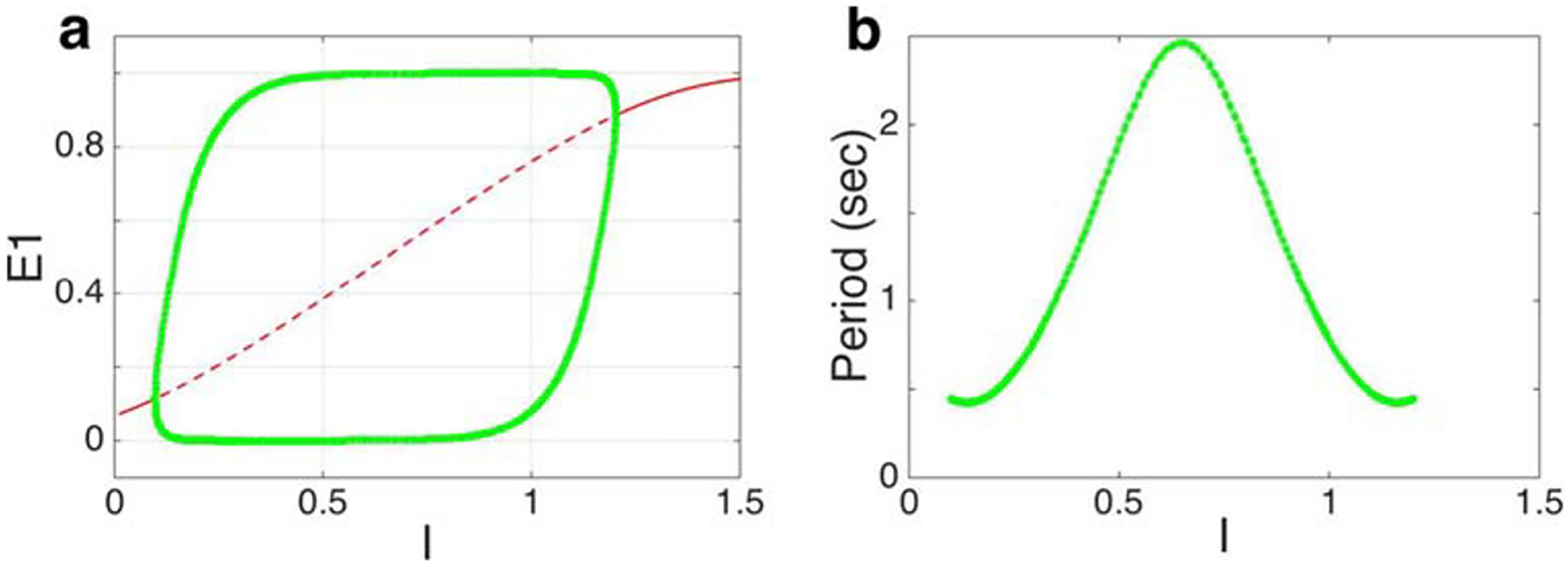
The hierarchical model captures conventional bistable binocular rivalry. a The bifurcation diagram with bifurcation parameter I when α = β = 0.3, and other parameters as in Fig. 3 shows the emergence and disappearance of periodic solutions. The green curves represent the branches of a stable periodic solution, the solid red curve represents a stable equilibrium, and the dashed red curve represents unstable equilibria; b The period of the corresponding stable periodic solution peaks around I = 0.6
3. Results
We use the hierarchical model described by Eq. (1) and Eq. (4) to explain the different experimentally observed features of multistable binocular rivalry involving interocular grouping. Moreover, we show that our model can provide a unifying mathematical framework that accounts for the generalized Levelt’s propositions, and provides concrete hypotheses of how different neural mechanisms shape perceptual dominance across levels of the visual hierarchy. At the same time, our model reduces to previous successful models of binocular rivalry with stimuli that conflict between the eyes, but do not promote inter-ocular grouping. We use numerical experiments and bifurcation theory to demonstrate the qualitative changes in the dynamics of the model to support these conclusions.
3.1. Levelt’s Propositions and their generalization
Levelt’s propositions relate stimulus strength to dominance duration – the time interval during which a single percept is reported; predominance – the fraction of the time a percept is reported; and alternation rate – the rate of switching between percept reports. Since the seminal work of Levelt (1965), there has been extensive work on extending the four original propositions (Shiraishi 1977; Bossink et al. 1993; Moreno-Bote et al. 2010; Platonov and Goossens 2013). In the context of bistable rivalry, the current version of Levelt’s propositions have most recently been summarized in a review paper of Brascamp et al. (2015) as: (I) Increasing the strength of the stimulus presented to one eye increases the predominance of that stimulus; (II) Increasing the difference in stimulus strengths between the two eyes increases the dominance duration of the stronger stimulus; (III) Increasing the difference in stimulus strengths between the two eyes reduces the perceptual alternation rate; (IV) Increasing stimulus strength in both eyes while keeping it equal between eyes increases the perceptual alternation rate. This effect may reverse at near-threshold stimulus strength (See Fig. 3 in Brascamp et al. (2015) for an illustration).
The strength of a percept has been defined as any attribute whose increase causes that percept to suppress the appearance of other percepts (Brascamp et al. 2015). Levelt’s Proposition I thus effectively defines the strength of a percept attribute according to whether it impacts a percept’s predominance. Jacot-Guillarmod et al. (2017) found experimental support for some of the following extensions of Levelt’s proposition using the stimuli and associated percepts shown in Fig. 1c, d:
Increasing percept strength of grouped percepts or single-eye percepts increases the perceptual predominance of those percepts. (Jacot-Guillarmod et al. 2017) showed that increasing color saturation increases the predominance of grouped percepts. Experimental results thus support this proposition, with color saturation defining the strength of the grouped percept class.
Decreasing the difference between the strength of the grouped percepts and that of single-eye percepts primarily decreases the average dominance duration of the stronger percepts. When the single-eye percept is stronger (weaker), increasing the strength of grouped percepts decreases (increases) the average dominance duration of the single-eye (grouped) percepts. Jacot-Guillarmod et al. (2017) showed that increasing color saturation primarily decreased the average dominance duration of the stronger, single-eye percepts, consistent with Proposition II. Experimental results did not speak to the validity of generalized Proposition II when the grouped percepts were stronger. When one class of percept is much stronger (e.g., single-eye percepts), we expect them to completely suppress percepts of the other class (e.g., grouped percepts). Percept strengths used in the experiments of Jacot-Guillarmod et al. (2017) were not sufficiently high to validate these predictions, but we test them in our model.
Decreasing the difference in strengths between grouped percepts and single-eye percepts increases the perceptual alternation rate. Since alternation rate and average dominance duration are related reciprocally, Proposition III follows from Proposition II.
Increasing the strength in both grouped percepts and single-eye percepts while keeping strength equal among percepts increases the perceptual alternation rate. Proposition IV was not tested directly in Jacot-Guillarmod et al. (2017), as changing color saturation affected the strengths of each percept differently. We show below that this Proposition holds in our model.
3.2. The hierarchical model exhibits perceptual multistabiliy
We first demonstrate how our model captures alternations between multiple percepts. As in previous studies, we associated a neural population with each percept: An elevation in the activity of a population at Level 2 of our model indicates that the corresponding percept is perceived and reported (Laing and Chow 2002; Wilson 2003; Moreno-Bote et al. 2007; Dayan 1998; Freeman 2005; Wilson 2009; Lehky 1988; Said and Heeger 2013; Lago-Fernandez and Deco 2002; Lumer 1998).
For a wide range of parameters, a single Level 2 neural population exhibited elevated activity, and suppressed the activity of the remaining populations (See Fig. 3a for a representative simulation). The order and timing of these periods of elevated firing were stochastic, and the distributions of the time periods of elevated firings were unimodal (Fig. 3b). This dynamics corresponded to the reports of experimental subjects who primarily reported seeing individual percepts over intervals of varying durations, and random alternations between the percepts. Consistent with previous models (Laing and Chow 2002; Wilson 2003; Moreno-Bote et al. 2007), stochastic alternations between percepts emerged due to the mutual suppression between the four populations at the second level of the hierarchy, while noise and adaptation drove alternations between the active populations.
Fig. 3.
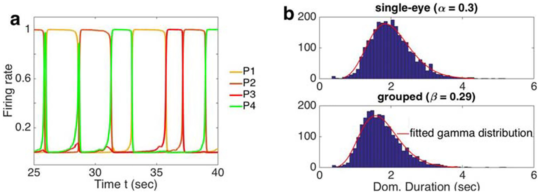
Dynamics of a hierarchical model of interocular grouping. a A typical time series of the firing rates, Pi, of neural populations at the second level of the model. Each of these populations is associated with one of the four percepts: P1 and P2 correspond to single-eye percepts, and P3 and P4 correspond to grouped percepts. Here we used same-eye coupling α = 0.3, interocular grouping strength β = 0.26, and input strength Ii = 1. b Distributions of dominance durations in the model have a single mode around 1.8s for single-eye percepts, and 1.5s for grouped percepts. These distributions are consistent with experimental data. Distributions were obtained from 100 time series, each 100s in duration. Parameters were set to Ii = 1.2, w = 1, g = 0.5, ci = 1, ν =γ = 0.45, κ = 0.5
3.3. Changing stimulus strength in the model yields experimentally observed dominance duration changes
In classical models of perceptual rivalry, stimulus and percept strengths are represented by the magnitude of input(s) to different neural populations. Changes in these input strengths correspond to changes in stimulus features like luminosity or contrast (Freeman 2005; Seely and Chow 2011). In the case of rivalry with grouped percepts (Fig. 1d), we assume that changes in color saturation have little effect on the strength of the inputs Ii (Jacot-Guillarmod et al. 2017). Rather, we assume that varying color saturation changes the tendency for interocular grouping between the two halves of images of the same color and orientation, consistent with Gestalt principles of similarity (Roelfsema 2006; Kohler 2015). Thus color saturation provides a visual cue for binding complementary halves of grouped percepts (Wagemans et al. 2012). We therefore modeled the effects of color saturation as a change in the strength of cross-hemispheric excitatory connections, β, between populations responding to like stimulus features. We also assumed that the excitatory coupling, α, between populations representing same-eye image halves was unaffected by changes in color saturation.
Jacot-Guillarmod et al. (2017) made several observations about the impact of color saturation on perceptual alternations recapitulated by our model. First, color saturation increased subjects’ predominance of grouped percepts (by 6% to 30%, see Fig. 4 of Jacot-Guillarmod et al. (2017) for more details), i.e. the fraction of the total time subjects reported a grouped percept out of the total time they reported seeing any percept: Increasing interocular coupling strength, β, in our model also increased the predominance of grouped percepts (See Fig. 4a). Thus color saturation, modeled by connection strength, β, between first level network populations in our model, satisfies the commonly used definition of stimulus strength (Brascamp et al. 2015).
Fig. 4.
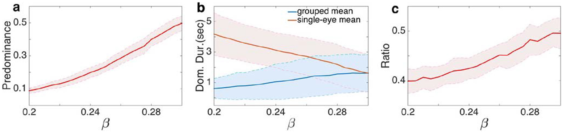
Effects of varying the interocular grouping strength, β, at the first level of the hierarchical model. a Predominance of grouped percepts increased with β. b The average dominance duration of single-eye percepts decreased with β, while that of grouped percepts remained approximately unchanged, particularly in the range 0.27 ≤ β ≤ 0.3. c Furthermore, the frequency of visits to grouped percepts increased with β. Other parameters were the same as in Fig. 3. Solid lines represent computationally obtained means, and shaded regions represent one standard deviation about the means obtained over 100 realizations
Second, Jacot-Guillarmod et al. (2017) observed that increasing color saturation decreased the average dominance duration (the average time the percept is seen before a switch occurs) of single-eye percepts while the average dominance duration of grouped percepts remained largely unchanged: the average dominance of single-eye percepts decreased by 0.09 to 0.23 and the change of the average dominance duration of grouped percepts ranged between −0.04 to 0.04, see Fig. 5 of Jacot-Guillarmod et al. (2017) for more details. Our model captured this feature over a range of parameters: For 0.2 < β < 0.3, increasing β decreased the dominance duration of single-eye percepts, while changes in dominance of grouped percepts were smaller and nearly absent as β approached α (See Fig. 4b).
Finally, (Jacot-Guillarmod et al. 2017) showed that increasing color saturation increased the ratio of visits to grouped percepts (by 3% to 32%, see Fig. 8 in Jacot-Guillarmod et al. (2017) for more details). Our model exhibited this behavior as well: The ratio of visits to grouped percepts increased with interocular grouping strength, β, (See Fig. 4c). As shown in Fig. 9 these results also hold in the presence of feedback.
Fig. 9.
Simulation results with feedback from the higher to the lower level of the hierarchy. Simulations indicate that the model can capture the key experimental results in Jacot-Guillarmod et al. (2017) even with feedback from the higher level to the lower level: a Predominance of grouped percepts increased as the interocular grouping strength increased; b The average dominance duration of single-eye percepts decreased while the average dominance duration of grouped percepts remained approximately unchanged (when β < α but close to the value α); c The ratio of the number of visits to the grouped percepts increased as the interocular grouping strength increased. Here ai = bi = 0.1 in Eq. (5), with other parameters as in Fig. 3
Note that our model only qualitatively matches the data. Due to experimental constraints, we obtained data at only two levels of color saturation. With our computational model we were able to change saturation over an entire interval. There is no precise match between the level of color saturation we used in the experiments, and that in the computational model. Any such correspondence is likely to vary between subjects, and possibly even between sessions with a single subject. We therefore did not attempt to specify the precise value of β that would correspond to our experimental data.
3.4. Neural population model conforms to the generalized Levelt’s propositions when α > β
We next asked whether the dynamics of our model agrees with experimentally observed generalizations of Levelt’s propositions (Jacot-Guillarmod et al. 2017). As shown in Fig. 4a, Proposition I does hold. In fact, this proposition holds over a wide range of parameter values, even when other propositions fail, and in all model versions we have explored.
We found that Proposition II holds in our model when β < α. When excitatory coupling between neural populations representing different-eye hemispheres is weaker than coupling between same-eye hemisphere populations, increasing interocular coupling strength β decreases the average dominance duration of the two single-eye percepts but very weakly increases the average dominance duration of the grouped percepts (See Fig. 4b). Since Proposition III follows from Proposition II and I, our model supports Proposition III as well.
To determine whether our model conforms to the prediction of Proposition IV, we varied α and β simultaneously while keeping them equal (See Fig. 5b). When grouping strength, β, is sufficiently high (β > 0.32), multiple sub-populations become co-active, indicating fusion. Figure 5b shows that an increase in β (and α) decreased the average dominance duration of both grouped and single-eye percepts, i.e. increasing the strengths of all percepts while keeping them equal increases the perceptual switching rate, in accord with Proposition IV. As in existing models for bistable binocular rivalry, Levelt’s Propositions IV holds only for parameter values over which the period of the periodic solutions of the associated deterministic model decreases as I increases (See Fig. 10 in Appendix for more details).
Fig. 5.
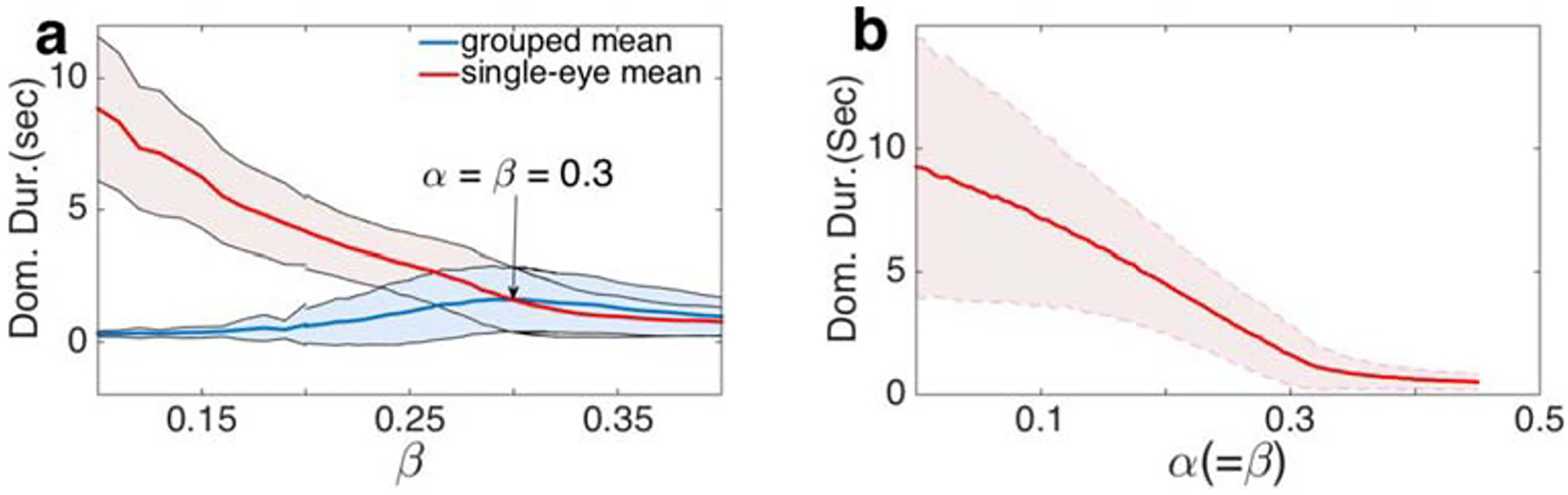
Levelt’s Proposition IV holds in the hierarchical model. a Proposition II held when β < α. Here α = 0.3, with other parameter values as in Fig. 3. b Increasing within- and between-eye grouping strengths (α and β respectively), simultaneously while keeping them equal decreased the average dominance duration
3.5. Generalized Levelt’s proposition II does not hold when α < β
To explore the full range of model behaviors, we also consider the case α < β representing strong interocular coupling. In this case, Proposition II fails since increasing the strength of the grouped percepts by increasing β does not lead to an increase in their average dominance duration, despite the grouped percepts being stronger (Fig. 5a). Such failures are common in other existing models when percept strengths are close (See Fig. 11c which reproduces results from Seely and Chow (2011)). Proposition II states that the average dominance duration of the stronger percept should change more than that of the weaker percept, but this effect does not hold when input strengths are close in mutual inhibitory models of perceptual bistability (Fig. 11c).
Fig. 11.
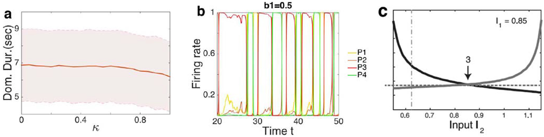
Adaptation rate, κ, at the higher level of the hieararchy, and top-down influence. a The adaptation rate had little or no effect on the dominance duration of percepts. Parameter values as in Fig. 3. b Example of top-down influence from only one percept, here P3 (a1 = a2 = b2 = 0 and b1 = 0.5). Top down input from one percept increased its dominance duration. Parameters not listed were as in Fig. 3. c Part of Fig. 4C from Seely and Chow (2011): Proposition IV did not hold when I2 ∈ (0.85, 1) since the increasing rate of the stronger percepts did not exceed the decreasing rate of the weak percept.
When the percept strength of the grouped percepts is much stronger than that of the single-eye percepts, perception is dominated by two rivaling grouped percepts. According to the original Levelt’s Proposition IV, further increasing in the strength of the grouped percepts should increase the switching rate between the two grouped percepts, reducing their average dominance duration. This is the case in our model, and is the reason for the decrease in average dominance duration when β > α shown in Fig. 5a, in contrast to the increase seen in Fig. 11c.
3.6. The mechanisms of multistable rivalry in the hierarchical model
We next describe the mechanisms that drive the perceptual switching dynamics in our model. The neural interactions implied by these mechanisms may underlie the dynamics described by the generalized Levelt’s Propositions:
Increasing interocular grouping strength, β, promotes co-activation of populations E1 and E4, as well as E2 and E3 at the first level of the hierarchy. Joint activity of populations E1 and E4 leads to increased activation of population P3 at the second level. Similarly, joint activity of E2 and E3 increases activation of P4. Due to mutual inhibition between populations at the same hemifields of opposite eyes, E1 and E3 (E2 and E4) synchronous activity of the pair E1 and E4 (E2 and E3) is likely not to be observed together with a coactivation of E1 and E2, or E3 and E4. Thus, a coactivation of the input E1E4 to P3 (E2E3 to P4) decreases the likelihood of elevated inputs E1E2 and E3E4 to the populations P1 and P2 corresponding to single-eye percepts. This explains why increasing interocular grouping strength, β, increases the predominance of the grouped percepts (P3 and P4), and hence the mechanism behind Proposition I.
As in earlier models of bistable rivalry, our hierarchical model exhibits perceptual switches either due to (a) inhibition release, or (b) escape driven by noise or the relaxation of adaptation (Curtu et al. 2008; Moreno-Bote et al. 2007). These two mechanisms are not mutually exclusive, and depend on model parameters. We chose parameters such that the escape mechanism dominates.
Keeping α = β and increasing their values is ‘equivalent’ to increasing the input, I: When single-eye percepts dominate, the two terms αE2 + βE4 ≈ α in the gain of E1 in Eq. (1a). A similar observation applies to the corresponding two terms determining the evolution of the firing rates E2, E3 and E4, and a similar effect occurs when the grouped percepts dominate. Hence, simultaneously increasing the value of α and β while keeping them equal, is approximately equivalent to increasing the input I. Since the period of the associated deterministic model decreases as input strength, I, increases in our chosen parameter range, we concluded that Proposition IV holds.
3.7. Impact of mutual inhibition at different levels of the hierarchical model
It has been debated at which level of the visual hierarchy mutually inhibitory interactions lead to rivalry (Carlson and He 2004; Andrew and Lotto 2004; Wilson 2003). Carlson and He (2004) showed that incompatibilities (conflicting interocular information that cannot be fused) at the lower level are necessary for producing rivalry. In contrast, Andrew and Lotto (2004) used identical stimuli within a different chromatic surround to show that the presence of rivalry can depend on the perceptual meaning of the visual stimuli, and must thus occur at higher levels of the visual processing hierarchy. Wilson (2003), on the other hand, used a two-stage feedforward model to show that the elimination of mutual inhibition at early stages reveals the activity at the higher layer, i.e. the activity remains at steady-state at the first level, and rivalry occurs only at the higher level.
Our model exhibits behavior similar to that reported by Wilson (2003): If lower-level mutual inhibition is not strong enough, activity at the lower level of the hierarchy approaches steady-state. Multistable rivalry in this situation requires stronger mutual inhibition at the higher level of the model. However, if this is the case, changes in interocular grouping strength have the same effect on all the percepts. As a consequence Levelt’s propositions do not hold. We conclude that multistable rivalry is possible with inhibition only at the higher level of the visual hierarchy. However, mutual inhibition at the lower level is necessary for generalized Levelt’s propositions to hold.
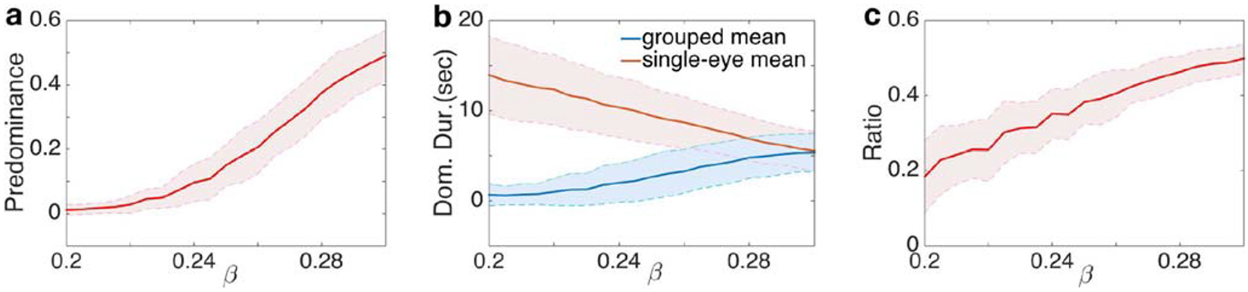
Next we asked whether mutual inhibition at the upper level is necessary for the generalized Levelt’s propositions to be hold. Our model showed that it was not. The four propositions hold without mutual inhibition at the upper level (Fig. 6): The predominance of the (weaker) grouped percepts increases with β (Fig. 6a), and the average dominance duration of the (stronger) single-eye percepts decreases faster than that of the (weaker) grouped percepts increases (Fig. 6b). The average dominance duration of all percepts decreases as α = β increases (Fig. 6c).
Fig. 6.
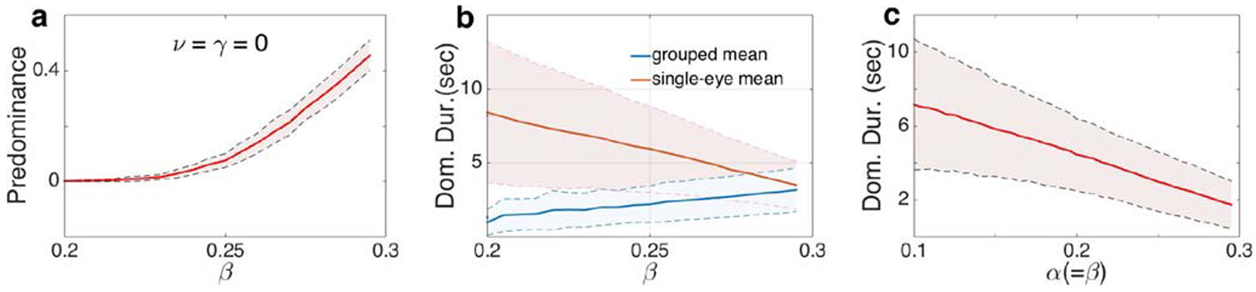
Levelt’s propositions hold without mutual inhibition at Level 2 (ν = γ = 0). a Predominance of grouped percepts increased with interocular grouping strength, β. b The average dominance duration of single-eye percepts (stronger percepts) decreased much faster than the average dominance duration of grouped percepts (weak percepts). c The average dominance duration decreased as α and β were increased and kept equal. Other parameter values as in Fig. 3
Weak or mild mutual inhibition at the upper level does help improve the persistence of dominant percepts by increasing the difference between the activity levels of the dominant and suppressed percepts. Nonetheless, dominance switches still tend to be mainly determined by the activity at the lower level (See Fig. 7), as the dominance of a percept becomes increasingly clear as mutual inhibition is increased.
Fig. 7.
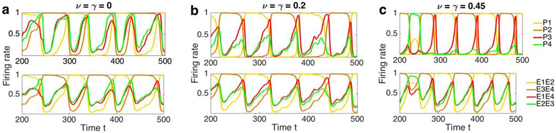
Time series with different mutual inhibition at the upper level. Each upper panel shows the neural activity of percepts (populations at the higher level of the hierarchy), and lower panels show inputs from the lower to the higher level of the hierarchical model; e.g., E1E2 is the input to P1. a, b Weak or mild mutual inhibition at the higher level helped disentangle different percepts, i.e. mutual inhibition at the upper level increased the distance between the activity levels of the dominating percepts and suppressed percepts; whereas c strong inhibition at the higher level lead to more frequent percept switching. Other parameter values as in Fig. 3
3.8. Impact of adaptation at the different levels
Adaptation plays a central role in most models of rivalry, by decreasing the stability of the dominant percept, and thus driving transitions between percepts (Kang and Blake 2010; Hollins and Hudnell 1980; Roumani and Moutoussis 2012; Blake and Overton 1979; Blake et al. 1990; van Boxtel et al. 2008; Wade and Weert 1986). We therefore asked at what level of the visual hierarchy this type of adaptation is needed to explain experimentally observed switching dynamics. As with mutual inhibition, we found that the generalized Levelt’s Propositions did hold when we removed adaptation (κ = 0) at the second level of the population model (See Fig. 8). In addition, a change in the strength of adaptation had little effect on the average dominance of either grouped percepts or single-eye percepts. See Fig. 11a for example. However, when we removed adaptation at the lower level, the activity of lower level populations approached steady state since adaptation was necessary for switching to occur, and the generalized propositions did not hold any more.
Fig. 8.
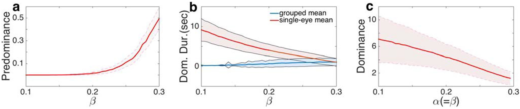
Generalized Levelt’s propositions hold in the absence of adaptation at the higher level of the visual hierarchy. a The predominance of grouped percepts increased with the interocular grouping strength, β. b The average dominance duration of single-eye percepts (stronger percepts) decreased much faster than the average dominance duration of grouped percepts (weak percepts). c The average dominance duration decreased with α and β when the two were kept equal. Parameter values as in Fig. 3
3.9. Impact of feedback
Thus far, we assumed an absence of feedback (ai = 0 and bi = 0) from the higher level of the visual hierarchy. However, numerous studies have found top–down feedback pathways from higher areas processing more complex features to lower areas processing basic geometric features (Angelucci et al. 2002; van Ee et al. 2006; Tong et al. 2006). Thus, we next asked whether generalized Levelt’s propositions still hold when we included feedback in our model as described in Eq. (5). Our simulations showed that for weak feedback (ai and bi small), the dynamics of the hierarchical model described above did not change qualitatively (Compare Fig. 9 with feedback, to Fig. 4 with no feedback). However, the average dominance duration was larger when we included feedback, consistent with findings in the bistable case (Wilson 2003).
3.10. The hierarchical model captures bistable binocular rivalry
As our hierarchical model is an extension of earlier models of binocular rivalry, we asked whether it also exhibits dynamics consistent with rivalry between two percepts. To answer this question we provided coherent “stimuli” to each pair of populations receiving input from the same eye, but conflicting stimuli to the two eyes. This would be equivalent to displaying a monochromatic square composed of vertical bars to one eye, and a monochromatic square composed of horizontal bars to the other eye.
Without feedback and inclusion of weak mutual inhibition and adaptation at the higher level, the dynamics of the system was mainly driven by the lower–level populations. Hence the only active populations at the higher level are therefore those corresponding to single–eye percepts. More precisely, without noise, and assuming I1 = I2, I3 = I4, the subsystem at the lower level has a flow-invariant subspace, S = {E1 = E2, E3 = E4, H1 = H2, H3 = H4}. Diekman et al. (2012) proved the subspace S is locally attracting at every point. When restricted to the subspace S, Eq. (1) reduces to a classical two population model (Laing and Chow 2002; Wilson 2003):
| (6) |
When population E1(= E2) dominates, it leads to the domination of percept 1 (P1). Similarly, when E3(= E4) dominates, then so does percept 2 (P2). Alternations in elevated activity between populations E1 and E3 therefore correspond to rivalry between percepts 1 and 2. Hence, Eq. (1) generalizes existing models of rivalry, and can capture features of binocular and multistable rivalry observed in experiments.
In addition, while the synchrony subspace S is associated with single-eye percepts (when E1 = E2 > E3 = E4, P1 dominates; when E3 = E4 > E1 = E2, P2 dominates), if I1 = I4, I2 = I3, then there is another synchrony subspace W = {E1 = E4, E2 = E3} (when I1 = I4, I2 = I3) associated to grouped percepts (when E1 = E4 > E3 = E2, P3 dominates; when E3 = E2 > E1 =E4, P4 dominates). The model thus also suggests that with sufficiently strong cues, the dynamics could be restricted to the invariant subset W, resulting in pure pattern rivalry.
4. Discussion
Multistable perceptual phenomena have long been used to probe the mechanisms underlying visual processing (Leopold and Logothetis 1999). Among these, binocular rivalry is perhaps the most robust, and has been studied most frequently. However, we can obtain different insights by employing visual inputs that are integrated to produce interocularly grouped percepts (Kovacs et al. 1996; Suzuki and Grabowecky 2002). These experiments are particularly informative when guided by Levelt’s Propositions, which were originally proposed to describe alternations between two rivaling percepts (Levelt 1965; Brascamp et al. 2015).
We generalized Levelt’s Propositions to perceptual multistability involving interocular grouping. These extended propositions are consistent with experimental findings, and the dynamics of a hierarchical model of visual processing. Our neural population model thus points to potential mechanisms that underlie experimentally reported perceptual alternations in rivalry with interocular grouping (Jacot-Guillarmod et al. 2017). In addition, there is no experimental data that we are aware of for the case of dominant grouped percepts. We found such percepts hard to achieve experimentally, but this does not mean that it is impossible to do so. Our computational results therefore offer a prediction that the proposition does not hold when grouped percepts are stronger.
Evidence suggests that rivalry exists across a hierarchy of visual cortical areas (Alias and Blake 2004). Indeed, rivalry can occur between complex stimulus representations, requiring higher order processing than typically observed in early visual areas (Kovacs et al. 1996; Tong et al. 2006). Physiological and imaging experiments have also shown that binocular rivalry modulates neural activities in the primary visual cortex, as well as higher areas including V2 and V4, MT, and inferior temporal cortex (Leopold and Logothetis 1996; Logothetis and Schall 1989; Sheinberg and Logothetis 1997; Tong et al. 1998). However, the way in which activity at these different levels contributes to binocular rivalry remains unclear. Competition at the lower or higher levels, or a combination thereof can all explain different aspects of this phenomenon, depending on the experiment (Leopold and Logothetis 1999; Pearson et al. 2007). Our model suggests that mutual inhibition at the early stages of the visual hierarchy is necessary for dynamics consistent with generalized Levelt’s Propositions.
Multistable rivalry has been studied previously using interocular grouping and fusion of coherently moving gratings. Moving plaid percepts arise when superimposing two drifting gratings moving at an angle to one another (Hupe and Rubin 2004). In these cases subjects perceive either a grating or a moving plaid in alternation (three total percepts: moving to the left, moving the right and moving upward). Mutual inhibitory, adapting neuronal network models display dynamics consistent with data from such experiments, suggesting the mechanisms behind such rivalry may be similar to those driving conventional binocular rivalry (Huguet et al. 2014). This provides further evidence that the classical models of rivalry can serve as a foundation for models describing more complex settings.
Comparisons with previous models of perceptual multistability
Our computational model is based on the assumption that perceptual multistability occurs via a winner-take-all process, with a single percept temporarily excluding all others (Wilson 2003; Shpiro et al. 2007). Consequently, some neural process must allow the system to switch from the dominant percept to another after a few seconds (Laing and Chow 2002). The simplest model of this process is a multistable system with slow adaptation and/or noise–driven switches between multiple attractors (Moreno-Bote et al. 2007; Braun and Mattia 2010). This framework is common in models of binocular rivalry (Laing and Chow 2002; Shpiro et al. 2007), non-eye-based perceptual rivalry (Brascamp et al. 2009)), and even perceptual multistability with more than two percepts (Diekman et al. 2013; Kilpatrick 2013; Huguet et al. 2014). Each percept typically corresponds to a single neural population which mutually inhibits the other(s). Spike rate adaptation or short term plasticity then drive the slow switching between network attractors (Laing and Chow 2002), and noise generates variation in the dominance times (Moreno-Bote et al. 2007).
Our computational model differs from previous ones in a few key ways. Excitatory connectivity at the first level facilitates both single-eye and grouped binocular percepts. Diekman et al. (2013) provided a preliminary account of interocular grouping, but ignored the effects of noise fluctuations on switching dynamics, and did not account for the known hierarchical structure of the visual system (Angelucci et al. 2002; Tong et al. 2006). In our model the strength of excitatory connectivity at the first level determines the input strength to populations at the higher level of the visual hierarchy, and ultimately each percept’s predominance. In this way, our model is similar to that of Wilson (2003) and Brascamp et al. (2013), who used a two level model to capture the effects of monocular and binocular neurons. Our model also includes feedback from the higher to the lower level, which could be due to attentional modulation. In this way, our model is similar in spirit to that of Li et al. (2017), who modeled attentional modulation of rivaling behavior. However, while previous models focused on the case of two possible percepts, our model accounts for four possible percepts in an interocular grouping task, and can be extended to include a larger number of percepts.
A number of other hierarchical models have also been proposed: Dayan (1998) developed a top-down statistical generative model, which places the competition at the higher level. Freeman (2005) proposed a feedforward multistage model with all stages possessing the same structure. These models also focused on conventional bistable binocular rivalry, and did not address the mechanisms of multistable rivalry.
Mutual inhibition.
Mutual inhibition is believed to account for the suppression of one percept by another in binocular rivalry. Most existing models of bistable binocular rivalry include only cross-eye mutual inhibition, but we note two exceptions: Brascamp et al. (2013) and Li et al. (2017) considered both cross-eye and same-eye inhibition to capture the rivalry emerging under rapid swapping of stimuli (two rival grating patches presented to alternate eyes rapidly). Under such rapid stimulus alternation neuronal populations from the same eye responding to orthogonal orientations at the same visual location could be active at the same time. Thus, same-eye inhibition between neuronal populations of the orthogonal orientations could affect perception. We note that neuronal populations responding to input from the same eye but different locations are co-activated in our model. However, as there are no conflicting stimuli appearing in rapid succession at the same location in our experiments, we did not include cross-orientation inhibition in our model.
Extensions to other computational models
We made several specific choices in our computational model. First, we described neural responses to input in each visual hemifield by a single variable. We could also have partitioned population activity based on orientation selectivity or receptive field location (Ferster and Miller 2000). This would allow us to describe the effects of horizontal connections that facilitate the representation of collinear orientation segments in more detail (Bosking et al. 1997; Angelucci et al. 2002). Since there is evidence for chromatically-dependent collinear facilitation (Beaudot and Mullen 2003), we could model the effects of image contrast and color saturation as separate contributions to interocular grouping. However, these extensions would complicate the model and make it more difficult to analyze. We therefore chose a reduced model with the effects of color saturation described by a single parameter, β.
Neural mechanisms of perceptual multistability
Our observations support the prevailing theory that perceptual multistability is significantly percept-based and involves higher visual and object-recognition areas (Leopold and Logothetis 1999). However, a number of issues remain unresolved. The question of whether and when binocular rivalry is eye-based or percept-based has not been fully answered (Blake 2001). Activity predictive of a subject’s dominant percept has been recorded in lateral geniculate nucleus (LGN) (Haynes and Rees 2005), primary visual cortex (V1) (Lee and Blake 2002; Polonsky et al. 2000), and higher visual areas (e.g., V2, V4, MT, IT) (Logothetis and Schall 1989; Leopold and Logothetis 1996; Sheinberg and Logothetis 1997). Thus, rivalry likely results from interactions between networks at several levels of the visual system (Freeman 2005; Wilson 2003). To understand how these activities collectively determine perception it is hence important to develop descriptive models that incorporate multiple levels of the visual processing hierarchy.
Collinear facilitation involves both recurrent connectivity in V1 as well as feedback connections from higher visual areas like V2 (Angelucci et al. 2002; Gilbert and Sigman 2007), reenforcing the notion that perceptual rivalry engages a distributed neural architecture. However, a coherent theory that relates image features to dominance statistics during perceptual switching is lacking. It is unclear how neurons that are associated to each subpopulation may interact due to grouping factors such as collinearity and color.
Conclusion
Our work supports the general notion that perceptual multistability is a distributed process that engages several layers of the visual system. Interocular grouping requires integration in higher visual areas (Leopold and Logothetis 1996), but orientation processing and competition occurs earlier in the visual stream (Angelucci et al. 2002; Gilbert and Sigman 2007). Overall, our model shows that the mechanisms that explain bistable perceptual rivalry can indeed be extended to multistable perceptual rivalry.
Acknowledgements
We thank Martin Golubitsky for helpful suggestions. Funding was provided by DHS-2014-ST-062-000057, NSF HRD-1800406 and NSF CNS-1831980 (YW); NSF DMS-1615737, NSF DMS-1853630 (ZPK); NIH-1R01MH115557 (KJ and ZPK); DBI-1707400 (KJ).
Appendix A: Choice of parameter values
We had to set a number of parameters in our model to capture the perceptual alternations observed experimentally. To do so we first let α = β, and chose a set of parameter values so that the corresponding deterministic model had a periodic solution with E1(t) = E2(t) and E3(t) = E4(t). i.e. the periodic solution associated with the alternation of single-eye percepts. We then used XPPAUT to obtain the bifurcation diagram shown in Fig. 10, where the green curve in (A) is a branch of stable periodic solutions and the green curve in (B) is the corresponding periods of the periodic solutions in (A). We choose the values of input strength Ii all to be equal and in the interval (0.8, 1.25) so that the model displayed decreases in dominance duration with increasing input strength I.
Changing the values of α and β changes the bifurcation diagram. However, by continuity, as long as parameter values are not far from those we used to obtain the bifurcation diagram, the dynamics of the system remains similar. In many of our simulations, we fixed the input values I to 1.2, and other values at α = 0.3, w = 1, g = 0.5, ci = 1, ν = γ = 0.45, κ = 0.5. τ = 10ms, τh = τa = 1000ms, δ = 0.03. The parameter values of w, g, ν, γ and κ roughly follow the values used in the literature (Seely and Chow 2011; Wilson 2003). We then numerically found the same qualitative results hold for I ∈ [1, 1.25].
Appendix B: Simulation procedure
To obtain the results shown in the figure, for each given parameter set we ran 100 realizations of the model for 300 seconds each and computed the dominance durations, predominance, and visit ratio for each percept. We pooled all dominance durations of one class of percepts (e.g., single-eye percepts or grouped percepts) and computed its average and standard deviation across occurrences and realizations.
Appendix C: Simulation results with feedback from higher to lower level
Our hierarchical model with sufficiently weak feedback from the higher level to the lower level can also capture the three main observations reported by Jacot-Guillarmod et al. (2017) with the minor difference that the average dominance duration increases (Fig. 9). Increasing the adaptation rate κ in the top level had little or no effect on the dominance duration of percepts (Fig. 11a shows single-eye percepts, but results for grouped percepts were similar) over a large interval (0, 0.8). The main effect of top down excitatory feedback from a percept we observed was to increase that percept’s dominance duration (Fig. 11b).
Footnotes
Conflict of interests The authors declare that they have no conflict of interest.
References
- Alias D, & Blake R (2004). Binocular rivalry. Cambridge: MIT Press. [Google Scholar]
- Andrew TJ, & Lotto RB (2004). Fusion and rivalry are dependent on the perceptual meaning of visual stimuli. Current Biology, 14, 418–423. [DOI] [PubMed] [Google Scholar]
- Angelucci A, Levitt JB, Walton EJ, Hupe JM, Bullier J, Lund JS (2002). Circuits for local and global signal integration in primary visual cortex. The Journal of Neuroscience, 22(19), 8633–8646. [DOI] [PMC free article] [PubMed] [Google Scholar]
- Arrington KF (1993). Neural network models for color brightness percception and binocular rivalry. PhD thesis, Boston University. [Google Scholar]
- Bartels A, & Logothetis NK (2010). Binocular rivalry: a time-depedence of eye and stimulus contributions. Journal of Vision, 10, 1–14. [DOI] [PubMed] [Google Scholar]
- Beaudot WH, & Mullen KT (2003). How long range is contour integration in human color vision? Visual Neuroscience, 20(01), 51–64. [DOI] [PubMed] [Google Scholar]
- Benda J, & Herz AV (2003). A universal model for spike-frequency adaptation. Neural Computation, 15(11), 2523–2564. [DOI] [PubMed] [Google Scholar]
- Blake R (1989). A neural theory of binocular rivalry. Psychological Review, 96, 145–167. [DOI] [PubMed] [Google Scholar]
- Blake R (2001). A primer on binocular rivalry, including current controversies. Brain and Mind, 2, 5–38. [Google Scholar]
- Blake R, & Logothetis NK (2002). Visual competition. Nature Reviews Neuroscience, 3, 13–21. [DOI] [PubMed] [Google Scholar]
- Blake R, & Overton R (1979). The site of binocular rivalry suppression. Perception, 8(2), 143–152. [DOI] [PubMed] [Google Scholar]
- Blake R, Westendorf D, Fox R (1990). Temporal perturbations of binocular rivalry. Perception & Psychophysics, 48(6), 593–602. [DOI] [PubMed] [Google Scholar]
- Bosking W, Zhang Y, Schofield B, Fitzpatrick D (1997). Orientation selectivity and the arrangement of horizontal connections in tree shrew striate cortex. Journal of Neuroscience, 17, 2112–2127. [DOI] [PMC free article] [PubMed] [Google Scholar]
- Bossink C, Stalmeier P, De Weert C (1993). A test of Levelt’s second proposition for binocular rivalry. Vision Research, 33(10), 1413–1419. [DOI] [PubMed] [Google Scholar]
- van Boxtel JJA, Alais D, van Ee R (2008). Retinotopic and non-retinotopic stimulus encoding in binocular rivalry and the involvement of feedback. Journal of Vision, 8(5), 17–17. [DOI] [PubMed] [Google Scholar]
- Brascamp J, Pearson J, Blake R, Van Den Berg A (2009). Intermittent ambiguous stimuli: Implicit memory causes periodic perceptual alternations. Journal of Vision, 9(3), 3. [DOI] [PMC free article] [PubMed] [Google Scholar]
- Brascamp J, Klink P, Levelt WJ (2015). The ‘laws’ of binocular rivalry: 50 years of Levelt’s propositions. Vision research, 109, 20–37. [DOI] [PubMed] [Google Scholar]
- Brascamp JW, Van RE, Noest AJ, Jacobs RH, van den Berg AV (2006). The time course of binocular rivalry reveals a fundamental role of noise. Journal of Vision, 6, 1244–1256. [DOI] [PubMed] [Google Scholar]
- Brascamp JW, Sohn H, Lee SH, Blake RH (2013). A monocular contribution to stimulus rivalry. PNAS. [DOI] [PMC free article] [PubMed] [Google Scholar]
- Braun J, & Mattia M (2010). Attractors and noise: twin drivers of decisions and multistability. NeuroImage, 52(3), 740–751. [DOI] [PubMed] [Google Scholar]
- Bressler DW, Denison RN, Silver MA (2013). The constitution of visual consciousness: lessons from binocular rivalry 90, 253. [Google Scholar]
- Brincat SL, & Connor CE (2006). Dynamic shape synthesis in posterior inferotemporal cortex. Neuron, 49(1), 17–24. [DOI] [PubMed] [Google Scholar]
- Carlson TA, & He S (2004). Competing global representations fail to initiate binocular rivalry. Neuron, 43, 970–914. [DOI] [PubMed] [Google Scholar]
- Curtu R, Shpiro A, Rubin N, Rinzel J (2008). Mechanisms for frequency control in neuronal competition models. SIAM J Appl Dyn Sys, 7, 609–649. [DOI] [PMC free article] [PubMed] [Google Scholar]
- Dayan P (1998). A hierarchical model of binocular rivalry. Neural Computation, 10, 1119–1135. [DOI] [PubMed] [Google Scholar]
- Diekman CO, Golubitsky M, McMillen T (2012). Reduction and dynamics of a generalized rivalry network with two learned patterns. SIAM J Appl Dyn Sys, 11, 1270–1309. [Google Scholar]
- Diekman CO, Golubitsky M, Wang Y (2013). Derived patterns in binocular rivalry networks. Journal of Mathematical Neuroscience,3(6). [DOI] [PMC free article] [PubMed] [Google Scholar]
- van Ee R, Noest AJ, Brascamp JW, van den Berg AV (2006). Attentional control over either of the two competing percepts of ambiguous stimuli revealed by a two-parameter analysis: Means do notmake the difference. Vision Research, 46, 3129–3141. [DOI] [PubMed] [Google Scholar]
- Faisal AA, Selen LPJ, Wolpert DM (2008). Noise in the nervous system. Nature Reviews Neuroscience, 9(4), 292–303. [DOI] [PMC free article] [PubMed] [Google Scholar]
- Ferster D, & Miller KD (2000). Neural mechanisms of orientation selectivity in the visual cortex. Annual Review of Neuroscience, 23(1), 441–471. [DOI] [PubMed] [Google Scholar]
- Freeman AW (2005). Multistage model for binocular rivalry. Journal of Neurophysiology, 94, 4412–4420. [DOI] [PubMed] [Google Scholar]
- Gilbert CD, & Sigman M (2007). Brain states: top-down influences in sensory processing. Neuron, 54(5), 677–696. [DOI] [PubMed] [Google Scholar]
- Golubitsky M, Zhao Y, Wang Y, Lu ZL (2019). The symmetry of generalized rivalry network models determines patterns of interocular grouping in four-location binocular rivalry. Journal of Neurophysiology. [DOI] [PMC free article] [PubMed] [Google Scholar]
- Häusser M, & Roth A (1997). Estimating the time course of the excitatory synaptic conductance in neocortical pyramidal cells using a novel voltage jump method. The Journal of Neuroscience, 17(20), 7606–7625. [DOI] [PMC free article] [PubMed] [Google Scholar]
- Haynes JD, & Rees G (2005). Predicting the stream of consciousness from activity in human visual cortex. Current Biology, 15(14), 1301–7. [DOI] [PubMed] [Google Scholar]
- Hollins M, & Hudnell K (1980). Adaptation of the binocular rivalry mechanism. Investigative Ophthalmology & Visual Science, 19(9), 1117–1120. [PubMed] [Google Scholar]
- Huguet G, Rinzel J, Hupé JM (2014). Noise and adaptation in multistable perception: Noise drives when to switch, adaptation determines percept choice. Journal of Vision, 14(3). [DOI] [PubMed] [Google Scholar]
- Hupe JM, & Rubin N (2004). The oblique plaid effect. Vision Research, 44(5), 489–500. [DOI] [PubMed] [Google Scholar]
- Jacot-Guillarmod A, Wang Y, Pedroza C, Ogmen H, Kilpatrick Z, Josić K (2017). Extending levelt’s propositions to perceptual multistability involving interocular grouping. Vision research, 133, 37–46. [DOI] [PubMed] [Google Scholar]
- Kalarickal GJ, & Marshall JA (2000). Neural model of temporal and stochastic properties of binocular rivalry. Neurocomputing, 32, 843–853. [Google Scholar]
- Kang MS, & Blake R (2010). What causes alternations in dominance during binocular rivalry? Atten Percept Psychophys, 72(1), 179–86. 10.3758/APP.72.1.179. [DOI] [PMC free article] [PubMed] [Google Scholar]
- Kilpatrick ZP (2013). Short term synaptic depression improves information transfer in perceptual multistability. Frontiers in Computational Neuroscience, 7(85). [DOI] [PMC free article] [PubMed] [Google Scholar]
- Kim CY, & Blake R (2007). Illusory color promotes interocular grouping during binocular rivalry. Psychonomic Bulletin & Review, 14(2), 356–362. [DOI] [PubMed] [Google Scholar]
- Klink PC, van Ee R, Nijs MM, Brouwer GJ, Noest AJ, van Wezel RJA (2008). Early interacions between neuronal adaptation and voluntary control determine perceptual choices in bistable vision. Journal of Vision, 8(16), 1–18. [DOI] [PubMed] [Google Scholar]
- Klink PC, Brascamp JW, Blake R, Wezel RJAV (2010). Experience-driven plasticity in binocular vision. Current Biology, 20. [DOI] [PMC free article] [PubMed] [Google Scholar]
- Kohler W (2015). The task of Gestalt psychology. Princeton: Princeton University Press. [Google Scholar]
- Kovacs I, Papathomas TV, Yang M, Feher A (1996). When the brain changes its mind: Interocular grouping during binocular rivalry. PNAS, 93, 15508–15511. [DOI] [PMC free article] [PubMed] [Google Scholar]
- Lago-Fernandez LF, & Deco G (2002). A model of binocular rivalry based on competition in it. Neurocomputing, 44–46, 503–507. [Google Scholar]
- Laing C, & Chow CC (2002). A spiking neuron model for binocular rivalry. J Comput Neurosci, 12, 39–53. [DOI] [PubMed] [Google Scholar]
- Lamme VA, & Roelfsema PR (2000). The distinct modes of vision offered by feedforward and recurrent processing. Trends in Neurosciences, 23(11), 571–579. [DOI] [PubMed] [Google Scholar]
- Lankheet MJM (2006). Unraveling adaptation and mutual inhibition in perceptual rivalry. Journal of Vision, 6, 304–310. 10.1167/6.4.1. [DOI] [PubMed] [Google Scholar]
- Lee SH, & Blake R (2002). V1 activity is reduced during binocular rivalry. Journal of Vision, 2(9), 4. [DOI] [PubMed] [Google Scholar]
- Lehky SR (1988). An astable multivibrator model of binocular rivalry. Perception, 17, 215–228. [DOI] [PubMed] [Google Scholar]
- Leopold D, & Logothetis NK (1999). Multistable phenomena: changing views in perception. Trends in Cognitive Sciences, 3, 254–264. [DOI] [PubMed] [Google Scholar]
- Leopold DA, & Logothetis NK (1996). Activity changes in early visual cortex refect monkeys’ percepts during binocular rivalry. Nature, 379, 549–553. [DOI] [PubMed] [Google Scholar]
- Levelt WJM (1965). On binocular rivalry. PhD thesis, Institute for Perception RVO-TNO Soeterberg; (Netherlands: ). [Google Scholar]
- Li HH, Rankin J, Rinzel J, Carrasco M, Heeger DJ (2017). Attention model of binocular rivalry. PNAS, 114(30). [DOI] [PMC free article] [PubMed] [Google Scholar]
- Logothetis NK, & Schall JD (1989). Neuronal correlates of subjective visual perception. Science, 245(4919), 761–763. [DOI] [PubMed] [Google Scholar]
- Lumer ED (1998). A neural model of binocular intergration and rivalry based on the coordination of action-potential timing in primary visual cortex. Cerebral Cortex, 8, 553–561. [DOI] [PubMed] [Google Scholar]
- Matsuoka K (1984). The dynamic model of binocular rivalry. Biological Cybernetics, 49, 201–208. [DOI] [PubMed] [Google Scholar]
- Moreno-Bote R, Rinzel J, Rubin N (2007). Noise-induced alternations in an attractor network model of perceptual bistability. Journal of Neurophysiology, 98, 1125–1139. [DOI] [PMC free article] [PubMed] [Google Scholar]
- Moreno-Bote R, Shapiro A, Rinzel J, Rubin N (2010). Alternation rate in perceptual bistability is maximal at and symmetric around equi-dominance. Journal of Vision, 10(11), 1–18. [DOI] [PMC free article] [PubMed] [Google Scholar]
- Noest AJ, van Ee R, Nijs MM, van Wezel RJA (2007). Percept-choice sequences driven by interrupted ambiguous stimuli: a low-levl neural model. Journal of Vision, 7(8), 1–14. [DOI] [PubMed] [Google Scholar]
- Pearson J, Tadin D, Blake R (2007). The effects of transcranial maganetic stimulation on visual rivalry. Journal of Vision, 7(7), 1–11. [DOI] [PubMed] [Google Scholar]
- Platonov A, & Goossens J (2013). Influence of contrast and coherence on the temporal dynamics of binocular motion rivalry. PloS One, 8(8), e71931. [DOI] [PMC free article] [PubMed] [Google Scholar]
- Polonsky A, Blake R, Braun J, Heeger D (2000). Neuronal activity in human primary visual cortex correlates with perception during binocular rivalry. Nature Neuroscience, 3, 1153–1159. [DOI] [PubMed] [Google Scholar]
- Ramachandran VS, Rao VM, Sriram S, Vidyasagar TR (1973). The role of colour perception and “pattern” recognition in stereopsis. Vision Research, 13, 505–509. [DOI] [PubMed] [Google Scholar]
- Renart A, De La Rocha J, Bartho P, Hollender L, Parga N, Reyes A, Harris KD (2010). The asynchronous state in cortical circuits. Science, 327(5965), 587–590. [DOI] [PMC free article] [PubMed] [Google Scholar]
- Riesenhuber M, & Poggio T (1999). Hierarchical models of object recognition in cortex. Nature Neuroscience, 2(11), 1019–1025. [DOI] [PubMed] [Google Scholar]
- Ringach DL, Hawken MJ, Shapley R, et al. (1997). Dynamics of orientation tuning in macaque primary visual cortex. Nature, 387(6630), 281–284. [DOI] [PubMed] [Google Scholar]
- Roelfsema PR (2006). Cortical algorithms for perceptual grouping. Annual Review of Neuroscience, 29, 203–227. [DOI] [PubMed] [Google Scholar]
- Roumani D, & Moutoussis K (2012). Binocular rivalry alternations and their relation to visual adaptation. Frontiers in Human Neuroscience, 6, 35–35. [DOI] [PMC free article] [PubMed] [Google Scholar]
- Said CP, & Heeger DJ (2013). A model of binocular rivalry and cross-orientation suppression. Plos Computational Biology, 9, e1002991. [DOI] [PMC free article] [PubMed] [Google Scholar]
- Salinas E, & Abbott L (1996). A model of multiplicative neural responses in parietal cortex. Proceedings of the National Academy of Sciences, 93(21), 11956–11961. [DOI] [PMC free article] [PubMed] [Google Scholar]
- Seely J, & Chow CC (2011). The role of mutual inhibition in binocular rivalry. Journal of Neurophysiology, 106, 2136–2150. [DOI] [PMC free article] [PubMed] [Google Scholar]
- Sheinberg DL, & Logothetis NK (1997). The role of temporal cortical areas in perceptual organization. Proceedings of the National Academy of Sciences, 94(7), 3408–3413. [DOI] [PMC free article] [PubMed] [Google Scholar]
- Shiraishi S (1977). A test of Levelt’s model on binocular rivalry. Japanese Psychological Research, 19(3), 129–135. [Google Scholar]
- Shpiro A, Curtu R, Rinzel J, Rubin N (2007). Dynamical characteristics common to neuronal competition models. Journal of Neurophysiology, 97(1), 462–473. [DOI] [PMC free article] [PubMed] [Google Scholar]
- Sincich LC, & Horton JC (2005). The circuitry of v1 and v2: integration of color, form, and motion. Annual Review of Neuroscience, 28, 303–326. [DOI] [PubMed] [Google Scholar]
- Sterzer P, Kleinschmit A, Rees G (2009). The neural bases of multistable perception. Trends in Cognitive Sciences, 13(7). [DOI] [PubMed] [Google Scholar]
- Stettler DD, Das A, Bennett J, Gilbert CD (2002). Lateral connectivity and contextual interactions in macaque primary visual cortex. Neuron, 36(4), 739–750. [DOI] [PubMed] [Google Scholar]
- Stollenwerk L, & Bode M (2003). Lateral neural model of binocular rivalry. Neural Computation, 15, 2863–2882. [DOI] [PubMed] [Google Scholar]
- Suzuki S, & Grabowecky M (2002). Evidence for perceptual “trapping” and adaptation in multistable binocular rivalry. Neuron, 36, 143–157. [DOI] [PubMed] [Google Scholar]
- Tong F (2001). Competing theories of binocular rivalry. Brain and Mind, 2, 55083. [Google Scholar]
- Tong F et al. (1998). Binocular rivalry and visual awareness in human extrastriate cortex. Neuron, 21(753–759). [DOI] [PubMed] [Google Scholar]
- Tong F, Meng M, Blake R (2006). Neural bases of binocular rivalry. Trends in Cognitive Sciences, 10,(11). [DOI] [PubMed] [Google Scholar]
- Wade NJ, & Weert CMMD (1986). Aftereffects in binocular rivalry. Perception, 15(4), 419–434. [DOI] [PubMed] [Google Scholar]
- Wagemans J, Elder JH, Kubovy M, Palmer SE, Peterson MA, Singh M, von der Heydt R (2012). A century of gestalt psychology in visual perception: I. perceptual grouping and figure–ground organization. Psychological Bulletin, 138(6), 1172. [DOI] [PMC free article] [PubMed] [Google Scholar]
- Wheatstone C (1838). Contributions to the physiology of vision. Part I. On some remarkable, and hitherto unobserved, phenomena of binocular vision. London and Edinburgh Philosophical Magazine and Journal of Science, 3, 241–267. [Google Scholar]
- Wilson HR (2003). Computational evidence for a rivalry hierarchy in vision. PNAS, 100, 14499–14503. [DOI] [PMC free article] [PubMed] [Google Scholar]
- Wilson HR (2007). Minimal physiological conditions for binocular rivalry and rivalry memory. Vision Res, 47, 2741–2750. [DOI] [PubMed] [Google Scholar]
- Wilson HR (2009). Requirements for conscious visual processing, Cambridge University Press, chap In Cortical Mechanisms of Vision, pp 399–417. [Google Scholar]