
Abstract
Polarization encoded images improve on conventional intensity imaging techniques by providing access to additional parameters describing the vector nature of light. In a polarimetric image, each pixel is related to a \(4 \times 1\) vector named Stokes vector (\(3 \times 1\) in a linear configuration, which is the framework retained afterwards). Such images comprise a valuable set of physical information on the objects they contain, amplifying subsequently the accuracy of the analysis that can be done. A Stokes imaging polarimeter yields data named radiance images from which Stokes vectors are reconstructed, supposed to comply with a physical admissibility constraint. Classical estimation techniques such as pseudo-inverse approach exhibit defects, hampering any relevant physical interpretation of the scene: (i) first, due to their sensitivity to noise and errors that may contaminate the observed radiance images and that may then propagate to the evaluation of the Stokes vector components, thus justifying an ad hoc a posteriori treatment of Stokes vectors; (ii) second, in not taking this physical admissibility criterion explicitly into account. Motivated by this observation, the proposed contribution aims to provide a method of reconstruction addressing both issues, thus ensuring smoothness and spatial consistency of the reconstructed components, as well as compliance with the prescribed physical admissibility constraint. A by-product of the algorithm is that the resulting angle of polarization reflects more faithfully the physical properties of the materials present in the image. The mathematical formulation yields a non-smooth convex optimization problem that is then converted into a min–max problem and solved by the generic Chambolle–Pock primal-dual algorithm. Several mathematical results (such as existence/uniqueness of the minimizer of the primal problem, existence of a saddle point to the associated Lagrangian, etc.) are supplied and highlight the well-posed character of the modelling. Experiments demonstrate that our method provides significant improvements (i) over the least square-based method both in terms of quantitative criteria (physical admissibility constraint automatically met) and qualitative assessment (spatial regularization/coherency), (ii) over the physical consistency of related relevant polarimetric parameters such as the angle and degree of polarization, (iii) robustness of the method when applied on real outdoor scenes acquired in degraded conditions (poor weather conditions, etc.).


References
Wolff, L.B., Andreou, A.G.: Polarization camera sensors. Image Vis. Comput. 13(6), 497–510 (1995)
Berger, K., Voorhies, R., Matthies, L.H.: Depth from stereo polarization in specular scenes for urban robotics. In: 2017 IEEE International Conference on Robotics and Automation (ICRA), pp. 1966–1973 (2017)
Zhu, D., Smith, W.A.P.: Depth From a Polarisation + RGB Stereo Pair. In: 2019 IEEE/CVF Conference on Computer Vision and Pattern Recognition (CVPR), pp. 7578–7587 (2019)
Morel, O., Stolz, C., Meriaudeau, F., Gorria, P.: Active lighting applied to three-dimensional reconstruction of specular metallic surfaces by polarization imaging. Appl. Opt. 45(17), 4062–4068 (2006)
Miyazaki, D., Saito, M., Sato, Y., Ikeuchi, K.: Determining surface orientations of transparent objects based on polarization degrees in visible and infrared wavelengths. J. Opt. Soc. Am. A 19(4), 687–694 (2002)
Rehbinder, J., Haddad, H., Deby, S., Teig, B., Nazac, A., Novikova, T., Pierangelo, A., Moreau, F.: Ex vivo Mueller polarimetric imaging of the uterine cervix: a first statistical evaluation. J. Biomed. Opt. 21(7), 1–8 (2016)
Wang, F., Ainouz, S., Meriaudeau, F., Bensrhair, A.: Polarization-based car detection. In: 2018 25th IEEE International Conference on Image Processing (ICIP), pp. 3069–3073 (2018)
Aycock, T.M., Chenault, D.B., Hanks, J.B., Harchanko, J.S.: Polarization-based mapping and perception method and system. Google Patents. US Patent 9,589,195 (2017)
Blin, R., Ainouz, S., Canu, S., Meriaudeau, F.: Road scenes analysis in adverse weather conditions by polarization-encoded images and adapted deep learning. In: 2019 IEEE Intelligent Transportation Systems Conference (ITSC), pp. 27–32 (2019)
Faisan, S., Heinrich, C., Rousseau, F., Lallement, A., Zallat, J.: Joint filtering estimation of Stokes vector images based on a nonlocal means approach. J. Opt. Soc. Am. A 29(9), 2028–2037 (2012)
Zallat, J., Heinrich, C.: Polarimetric data reduction: a Bayesian approach. Opt. Express 15(1), 83–96 (2007)
Zallat, J., Heinrich, C., Petremand, M.: A Bayesian approach for polarimetric data reduction: the Mueller imaging case. Opt. Express 16(10), 7119–7133 (2008)
Valenzuela, J.R., Fessler, J.A.: Joint reconstruction of Stokes images from polarimetric measurements. J. Opt. Soc. Am. A 26(4), 962–968 (2009)
Chambolle, A., Pock, T.: A first-order primal-dual algorithm for convex problems with applications to imaging. J. Math. Imaging Vis. 40(1), 120–145 (2011)
Bass, M., Van Stryland, E.W., Williams, D.R., Wolfe, W.L.: Handbook of Optics, Third Edition Volume II: Design, Fabrication and Testing, Sources and Detectors, Radiometry and Photometry, 3rd edn. McGraw-Hill, Inc., New York (2009)
Terrier, P., Devlaminck, V.: Robust and accurate estimate of the orientation of partially polarized light from a camera sensor. Appl. Opt. 40(29), 5233–5239 (2001)
Ainouz, S., Morel, O., Fofi, D., Mosaddegh, S., Bensrhair, A.: Adaptive processing of catadioptric images using polarization imaging: towards a pola-catadioptric model. Opt. Eng. 52(3), 1–9 (2013)
Zubko, E., Chornaya, E.: On the ambiguous definition of the degree of linear polarization. Res. Notes AAS 3(3), 45 (2019)
Wang, Z., Zheng, Y., Chuang, Y.-Y.: Polarimetric camera calibration using an LCD monitor. In: 2019 IEEE/CVF Conference on Computer Vision and Pattern Recognition (CVPR), pp. 3738–3747 (2019)
Chambolle, A.: An algorithm for total variation minimization and applications. J. Math. Imaging Vis. 20(1), 89–97 (2004)
Pierre, F., Aujol, J.-F., Bugeau, A., Papadakis, N., Ta, V.-T.: Luminance-chrominance model for image colorization. SIAM J. Imaging Sci. 8(1), 536–563 (2015)
Azé, D.: Éléments d’analyse convexe et variationnelle. Mathématiques pour le \(2^{{\grave{{\rm e}}{{\rm me}}}}\) cycle. Ellipses, Paris (1997)
Ekeland, I., Témam, R.: Convex Analysis and Variational Problems. Society for Industrial and Applied Mathematics, Philadelphia (1999)
Moreau, J.-J.: Fonctions convexes duales et points proximaux dans un espace hilbertien. C. R. Acad. Sci. 255, 2897–2899 (1962)
Combettes, P.L., Pesquet, J.-C.: Proximal splitting methods in signal processing. In: Bauschke, H.H., Burachik, R.S., Combettes, P.L., Elser, V., Luke, D.R., Wolkowicz, H. (eds.) Fixed-Point Algorithms for Inverse Problems in Science and Engineering, pp. 185–212. Springer, New York (2011)
Kolmogorov, A., Fomine, S.: Éléments de la Théorie des Fonctions et de l’Analyse Fonctionnelle, 2nd edn. Mir, Moscow (1977)
Tang, L., Fang, Z.: Edge and contrast preserving in total variation image denoising. EURASIP J. Adv. Signal Process. 2016, 1–21 (2016)
Wang, F., Ainouz, S., Petitjean, C., Bensrhair, A.: Specularity removal: a global energy minimization approach based on polarization imaging. Comput. Vis. Image Underst. 158, 31–39 (2017)
Wang, Y., Jiang, Z., Shi, J.: Highlight area inpainting guided by illumination model. In: Fifth International Conference on Graphic and Image Processing (ICGIP 2013), vol. 9069, p. 90691 (2014). International Society for Optics and Photonics
Kupinski, M.K., Bradley, C.L., Diner, D.J., Xu, F., Chipman, R.A.: Angle of linear polarization images of outdoor scenes. Opt. Eng. 58(8), 082419 (2019)
Baek, S.-H., Jeon, D.S., Tong, X., Kim, M.H.: Simultaneous acquisition of polarimetric SVBRDF and normals. ACM Trans. Graph. 37(6) (2018)
Schechner, Y.Y., Narasimhan, S.G., Nayar, S.K.: Polarization-based vision through haze. Appl. Opt. 42(3), 511–525 (2003)
Sarafraz, A., Negahdaripour, S., Schechner, Y.Y.: Enhancing images in scattering media utilizing stereovision and polarization. In: 2009 Workshop on Applications of Computer Vision (WACV), pp. 1–8 (2009). IEEE
Beck, A.: First-Order Methods in Optimization. Society for Industrial and Applied Mathematics, Philadelphia (2017)
Acknowledgements
This project was co-financed by the European Union with the European regional development fund (ERDF, 18P03390/ 18E01750/18P02733), by the Haute-Normandie Régional Council via the M2SINUM project and by the French Research National Agency ANR via ICUB project ANR 17-CE 22-0011-01. The authors would like to thank Dr Sylvain Faisan (ICube - MIV, Université de Strasbourg) for providing us with the code to generate artificial data in the full Stokes recovery case.
Author information
Authors and Affiliations
Corresponding author
Additional information
Publisher's Note
Springer Nature remains neutral with regard to jurisdictional claims in published maps and institutional affiliations.
Appendices
Appendix A: Pointwise Infimum of Concave Functions
Let us denote by \(f(p)=\displaystyle {\inf _{S\in {\mathcal {K}}}}\,{\mathcal {L}}(S,p)=\displaystyle {\inf _{S\in {\mathcal {K}}}}\,{\mathcal {L}}_S(p)\). In our case, for each p the infimum is reached so that we could write equivalently \(f(p)=\displaystyle {\min _{S\in {\mathcal {K}}}}\,{\mathcal {L}}_{S}(p)\). Let us prove that f is concave.
We recall a preliminary result.
Theorem 3
Let X be a set and let \(f : X \rightarrow \bar{{\mathbb {R}}}\). The hypograph of f is defined by
A function \(f: X \rightarrow \bar{{\mathbb {R}}}\) is concave if and only if its hypograph is convex.
Coming back to our problem,
which is convex as the intersection of convex sets.
Appendix B: Pointwise Infimum of Continuous Functions
Theorem 4
Let \((X,\tau )\) be a topological space and let \(f : X \rightarrow \bar{{\mathbb {R}}}\) be a function. Function f is upper semi-continuous if \(\forall \alpha \in {\mathbb {R}}\), the set \(\left\{ x\in X\,\mid \,f(x)<\alpha \right\} \) is open.
Let us prove that \(f : p \in {\mathcal {B}} \mapsto \displaystyle {\inf _{S\in {\mathcal {K}}}}\,{\mathcal {L}}(S,p)\) is upper semi-continuous. Let \(\alpha \in {\mathbb {R}}\). Let \(p\in f^{-1}((-\infty ,\alpha ))\). Then, \(\displaystyle {\inf _{S\in {\mathcal {K}}}}\,{\mathcal {L}}(S,p)<\alpha \) and there exists \({\bar{S}}_p\in {\mathcal {K}}\) such that \({\mathcal {L}}({\bar{S}}_p,p)={\mathcal {L}}_{{\bar{S}}_p}(p)<\alpha \). This implies that
which is open as the union of open sets.
Appendix C: Alternative Proof to Get the Proximal Operator of \(\tau \, g\)
Consider the three-dimensional optimization problem
Using the identity
and the fact that \(A^TA=\begin{pmatrix}1&{}0&{}0\\ 0&{}\frac{1}{2}&{}0\\ 0&{}0&{}\frac{1}{2} \end{pmatrix}\), the minimization problem can be equivalently restated as:
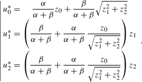
with \(\left\{ \begin{array}{cccc} \alpha &{}=&{}\frac{1}{2\tau }+\frac{\mu }{2}\\ \beta &{}=&{}\frac{1}{2\tau }+\frac{\mu }{4} \end{array}\right. \), and \(z_0=\frac{\frac{1}{2\tau }u_0+\frac{\mu }{2}b_0}{\alpha }\), \(z_1=\frac{\frac{1}{2\tau }u_1+\frac{\mu }{2}b_1}{\beta }\) and \(z_2=\frac{\frac{1}{2\tau }u_2+\frac{\mu }{2}b_2}{\beta }\).
We then set \(\left\{ \begin{array}{ccc}{\bar{u}}_0&{}=&{}\sqrt{\alpha }\,{\tilde{u}}_0\\ {\bar{u}}_1&{}=&{}\sqrt{\beta }\,{\tilde{u}}_1\\ {\bar{u}}_2&{}=&{}\sqrt{\beta }\,{\tilde{u}}_2 \end{array}\right. \), \(\left\{ \begin{array}{ccc}{\bar{z}}_0&{}=&{}\sqrt{\alpha }\,z_0\\ {\bar{z}}_1&{}=&{}\sqrt{\beta }\,z_1\\ {\bar{z}}_2&{}=&{}\sqrt{\beta }\,z_2 \end{array}\right. \) and \(\overline{{\mathcal {C}}}\) the closed convex set defined by
and consider the auxiliary problem related to (C1)
which thus amounts to computing the projection of \({\bar{z}}=({\bar{z}}_0,{\bar{z}}_1,{\bar{z}}_2)\) onto \(\overline{{\mathcal {C}}}\). Once the (unique) solution of (C2) is obtained, it suffices to use the previous change of variable to recover the \(u^{*}_i\)’s.
Let us now recall the following result dedicated to orthogonal projection onto epigraphs.
Theorem 5
Orthogonal projection onto epigraphs, taken from [34, Chapter 6, Theorem 6.36] with \({\mathbb {E}}\) a Euclidean space, let
where \(g : {\mathbb {E}} \rightarrow {\mathbb {R}}\) is convex. Then,
where \(\lambda ^{*}\) is any positive root of the function
In addition, \(\Psi \) is nonincreasing.
We invoke the previous theorem with \(g(\cdot )=\sqrt{\frac{\alpha }{\beta }}\,\Vert \cdot \Vert _{{\mathbb {R}}^2}\) to obtain the formula and follow the arguments of Beck ([34, Chapter 6]) (we respect the same order in the arguments of \(P_{\overline{{\mathcal {C}}}}(\cdot )\) as in [34])
where \(\lambda ^{*}\) is any positive root of the function \(\Psi (\lambda )=\sqrt{\frac{\alpha }{\beta }}\,\Vert {\text{ prox }}_{\lambda \,\sqrt{\frac{\alpha }{\beta }}\Vert \cdot \Vert _{{\mathbb {R}}^2}}({\hat{z}})\Vert _{{\mathbb {R}}^2}-\lambda -{\bar{z}}_0\).
Let \(({\hat{z}},\bar{z_0})\) be such that \({\bar{z}}_0 <\sqrt{\frac{\alpha }{\beta }}\,\Vert {\hat{z}}\Vert _{{\mathbb {R}}^2}\).
Recall that
Plugging the above into the expression of \(\Psi \) leads to
The unique positive root \(\lambda ^{*}\) of the piecewise linear function \(\Psi \) is
resulting in

If we summarize the whole results, coming back to the initial variables, we see that we recover the results obtained with the necessary and sufficient KKT condition. Indeed,
-
If \({\bar{z}}_0 \ge \sqrt{\frac{\alpha }{\beta }}\,\Vert {\hat{z}}\Vert _{{\mathbb {R}}^2}\) or equivalently, \(z_0\ge \sqrt{z_1^2+z_2^2}\),
$$\begin{aligned}&\left( \sqrt{\alpha }u^{*}_0,\sqrt{\beta }u^{*}_1,\sqrt{\beta }u^{*}_2 \right) =({\bar{z}}_0,{\bar{z}}_1,{\bar{z}}_2)\\&\quad =\left( \sqrt{\alpha }z_0,\sqrt{\beta }z_1,\sqrt{\beta }z_2\right) , \end{aligned}$$yielding
$$\begin{aligned} \left( u^{*}_0,u^{*}_1,u^{*}_2 \right) =(z_0,z_1,z_2). \end{aligned}$$ -
If \({\bar{z}}_0 <\sqrt{\frac{\alpha }{\beta }}\,\Vert {\hat{z}}\Vert _{{\mathbb {R}}^2}\) or equivalently, \(z_0< \sqrt{z_1^2+z_2^2}\),
-
(i)
If \({\bar{z}}_0 \ge 0\) (or equivalently \(z_0\ge 0\)), then \(\Vert {\hat{z}}\Vert _{{\mathbb {R}}^2}\ge -{\bar{z}}_0\sqrt{\frac{\alpha }{\beta }}\) or equivalently \(\beta \,\sqrt{z_1^2+z_2^2}\ge -\alpha \,z_0\), and intermediate computations lead to
-
(ii)
If \({\bar{z}}_0<0\) (or equivalently, \(z_0<0\)) and \(\Vert {\hat{z}}\Vert _{{\mathbb {R}}^2}<-{\bar{z}}_0\sqrt{\frac{\alpha }{\beta }}\) or equivalently \(\beta \,\sqrt{z_1^2+z_2^2}< -\alpha \,z_0\), then
$$\begin{aligned} \left( u^{*}_0,u^{*}_1,u^{*}_2 \right) =(0,0,0). \end{aligned}$$ -
(iii)
If \({\bar{z}}_0<0\) (or equivalently, \(z_0<0\)) and \(\Vert {\hat{z}}\Vert _{{\mathbb {R}}^2}\ge -{\bar{z}}_0\sqrt{\frac{\alpha }{\beta }}\) or equivalently \(\beta \,\sqrt{z_1^2+z_2^2}\ge -\alpha \,z_0\), then intermediate computations lead to


Rights and permissions
Springer Nature or its licensor (e.g. a society or other partner) holds exclusive rights to this article under a publishing agreement with the author(s) or other rightsholder(s); author self-archiving of the accepted manuscript version of this article is solely governed by the terms of such publishing agreement and applicable law.
About this article

Cite this article
Le Guyader, C., Ainouz, S. & Canu, S. A Physically Admissible Stokes Vector Reconstruction in Linear Polarimetric Imaging. J Math Imaging Vis 65, 592–617 (2023). https://doi.org/10.1007/s10851-022-01139-2
Received:
Accepted:
Published:
Issue Date:
DOI: https://doi.org/10.1007/s10851-022-01139-2