
Abstract
We consider scenario approximation of problems given by the optimization of a function over a constraint that is too difficult to be handled but can be efficiently approximated by a finite collection of constraints corresponding to alternative scenarios. The covered programs include min-max games, and semi-infinite, robust and chance-constrained programming problems. We prove convergence of the solutions of the approximated programs to the given ones, using mainly epigraphical convergence, a kind of variational convergence that has demonstrated to be a valuable tool in optimization problems.


Notes
This object is also called essential intersection, but this name is quite misleading since it induces some confusion with the ℙ-essential intersection.
It is enough to take f(x,y)=1−2⋅1{(x,y)∈A}, where 1{z∈B} is the indicator or characteristic function, that is the function taking the value 1 if z∈B and 0 otherwise.
Some of them are discussed in [3, pp. 99–100].
χ is defined as:
$$\chi (x,C )=\left \{ \begin{array}{l@{\quad}l} 0, & \textrm{if}\ x\in C\\ +\infty, & \textrm{if }x\notin C\end{array} \right .,\quad x\in\mathbf{X}. $$This is similar to the program considered in [25].
It would be clearly possible to explicitly consider two different approximating programs, one for the deterministic and one for the stochastic case. However, the separation between the two programs is quite artificial. As an example, also for (7) it is possible to define a fictitious probability measure on Y and to draw random points according to it. Provided the density of the measure is strictly positive, the behavior of the solutions is described by Corollary 5.2.
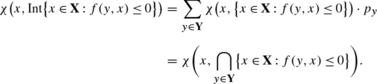
This can be simply verified using the result of [18] quoted in the proof of Corollary 5.2. Indeed, if (p y ) are the probability masses, we have

References
Still, G.: Discretization in semi-infinite programming: The rate of convergence. Math. Program., Ser. A 91(1), 53–69 (2001)
Calafiore, G., Campi, M.C.: Robust convex programs: Randomized solutions and applications in control. In: Proceedings of the 42nd IEEE Conference on Decision and Control, Maui, Hawaii, USA, December 2003 pp. 2423–2428 (2003)
Campi, M.C., Calafiore, G.: Decision making in an uncertain environment: The scenario-based optimization approach. In: Kárný, M., Kracík, J., Andrýsek, J. (eds.) Multiple participant decision making. International Series on Advanced Intelligence, vol. 9, pp. 99–111. Advanced Knowledge International (2004)
Calafiore, G., Campi, M.C.: Uncertain convex programs: Randomized solutions and confidence levels. Math. Program. 102, 25–46 (2005)
Nemirovski, A., Shapiro, A.: Scenario approximations of chance constraints. In: Calafiore, G., Dabbene, F. (eds.) Probabilistic and Randomized Methods for Design under Uncertainty, pp. 3–48. Springer, Berlin (2006)
Pucci de Farias, D., Van Roy, B.: On constraint sampling in the linear programming approach to approximate dynamic programming. Math. Oper. Res. 29(3), 462–478 (2004)
Reemtsen, R.: Semi-infinite programming: Discretization methods. In: Floudas, C., Pardalos, P. (eds.) Encyclopedia of Optimization, pp. 3417–3424. Springer, New York (2009)
Reemtsen, R.: Discretization methods for the solution of semi-infinite programming problems. J. Optim. Theory Appl. 71(1), 85–103 (1991)
Reemtsen, R.: Some outer approximation methods for semi-infinite optimization problems. J. Comput. Appl. Math. 53(1), 87–108 (1994)
Combettes, P.: Strong convergence of block-iterative outer approximation methods for convex optimization. SIAM J. Control Optim. 38(2), 538–565 (2000) (electronic)
Shapiro, A.: Monte Carlo sampling methods. In: Stochastic programming. Handbooks Oper. Res. Management Sci., vol. 10, pp. 353–425. Elsevier, Amsterdam (2003)
Huber, P.J.: The 1972 Wald lecture. Robust statistics: A review. Ann. Math. Stat. 43, 1041–1067 (1972)
Niederreiter, H.: Random number generation and quasi-Monte Carlo methods. CBMS-NSF Regional Conference Series in Applied Mathematics, vol. 63. Society for Industrial and Applied Mathematics (SIAM), Philadelphia (1992)
Polak, E.: On the mathematical foundations of nondifferentiable optimization in engineering design. SIAM Rev. 29(1), 21–89 (1987)
Hettich, R., Kortanek, K.O.: Semi-infinite programming: Theory, methods, and applications. SIAM Rev. 35(3), 380–429 (1993)
Žaković, S., Rustem, B.: Semi-infinite programming and applications to minimax problems. Ann. Oper. Res. 124, 81–110 (2003)
Hess, C., Seri, R., Choirat, C.: Approximations results for robust optimization. Working paper (2010)
Hiriart-Urruty, J.B.: Contributions à la programmation mathématique: cas déterministe et stochastique. Ph.D. thesis, Université de Clermont-Ferrand II, Clermont (1977)
Charnes, A., Cooper, W.W., Symonds, G.H.: Cost horizons and certainty equivalents: An approach to stochastic programming of heating oil. Manag. Sci. 4, 183–195 (1958)
Charnes, A., Cooper, W.W.: Chance-constrained programming. Manag. Sci. 6, 73–79 (1959/1960)
Charnes, A., Cooper, W.W.: Chance constraints and normal deviates. J. Am. Stat. Assoc. 57, 134–148 (1962)
Sengupta, J.K.: Stochastic linear programming with chance constraints. Int. Econ. Rev. 11, 101–116 (1970)
Still, G.: Generalized semi-infinite programming: Theory, methods. Eur. J. Oper. Res. 119, 301–313 (1999)
Still, G.: Generalized semi-infinite programming: Numerical aspects. Optimization 49(3), 223–242 (2001)
Bai, D., Carpenter, T.J., Mulvey, J.M.: Making a case for robust models. Manag. Sci. 43, 895–907 (1997)
Redaelli, G.: Convergence problems in stochastic programming models with probabilistic constraints. Riv. Mat. Sci. Econ. Soc. 21(1–2), 147–164 (1998)
Pennanen, T., Koivu, M.: Epi-convergent discretizations of stochastic programs via integration quadratures. Numer. Math. 100, 141–163 (2005)
Choirat, C., Hess, C., Seri, R.: A functional version of the Birkhoff ergodic theorem for a normal integrand: A variational approach. Ann. Probab. 31(1), 63–92 (2003)
Choirat, C., Hess, C., Seri, R.: Approximation of stochastic programming problems. In: Niederreiter, H., Talay, D. (eds.) Monte Carlo and Quasi-Monte Carlo Methods 2004, pp. 45–60. Springer, Berlin (2006)
Dal Maso, G.: An Introduction to Γ-Convergence. Progress in Nonlinear Differential Equations and their Applications, vol. 8. Birkhäuser, Boston (1993)
Jagannathan, R.: Chance-constrained programming with joint constraints. Oper. Res. 22(2), 358–372 (1974)
López, M., Still, G.: Semi-infinite programming. Eur. J. Oper. Res. 180(2), 491–518 (2007)
Rockafellar, R.T., Wets, R.J.B.: Variational Analysis. Grundlehren der Mathematischen Wissenschaften [Fundamental Principles of Mathematical Sciences], vol. 317. Springer, Berlin (1998)
Allen, F.M., Braswell, R.N., Rao, P.V.: Distribution-free approximations for chance constraints. Oper. Res. 22(3), 610–621 (1974)
Gray, R.M., Kieffer, J.C.: Asymptotically mean stationary measures. Ann. Probab. 8(5), 962–973 (1980)
Wets, R.J.B.: Stochastic programs with chance constraints: Generalized convexity and approximation issues. In: Generalized Convexity, Generalized Monotonicity: Recent Results, Luminy, 1996. Nonconvex Optim. Appl., vol. 27, pp. 61–74. Kluwer Academic, Dordrecht (1998)
Pagnoncelli, B.K., Ahmed, S., Shapiro, A.: Sample average approximation method for chance constrained programming: Theory and applications. J. Optim. Theory Appl. 142(2), 399–416 (2009)
Elker, J., Pollard, D., Stute, W.: Glivenko–Cantelli theorems for classes of convex sets. Adv. Appl. Probab. 11(4), 820–833 (1979)
Steele, J.M.: Empirical discrepancies and subadditive processes. Ann. Probab. 6(1), 118–127 (1978)
Shorack, G.R., Wellner, J.A.: Empirical Processes with Applications to Statistics. Wiley Series in Probability and Mathematical Statistics: Probability and Mathematical Statistics. Wiley, New York (1986)
Nobel, A.: A counterexample concerning uniform ergodic theorems for a class of functions. Stat. Probab. Lett. 24(2), 165–168 (1995)
Henrion, R., Römisch, W.: Metric regularity and quantitative stability in stochastic programs with probabilistic constraints. Math. Program., Ser. A 84(1), 55–88 (1999)
Luedtke, J., Ahmed, S.: A sample approximation approach for optimization with probabilistic constraints. SIAM J. Optim. 19(2), 674–699 (2008)
Cheney, E.W.: Introduction to Approximation Theory. AMS Chelsea, Providence (1998). Reprint of the second (1982) edition
Barrodale, I., Phillips, C.: Algorithm 495: Solution of an overdetermined system of linear equations in the Chebyshev norm. ACM Trans. Math. Softw. 1(3), 264–270 (1975)
Devroye, L.: Laws of the iterated logarithm for order statistics of uniform spacings. Ann. Probab. 9(5), 860–867 (1981)
Aliprantis, C.D., Border, K.C.: Infinite-Dimensional Analysis. Springer, Berlin (1999)
Beer, G., Rockafellar, R.T., Wets, R.J.B.: A characterization of epi-convergence in terms of convergence of level sets. Proc. Am. Math. Soc. 116(3), 753–761 (1992)
Molchanov, I.S.: A limit theorem for solutions of inequalities. Scand. J. Stat. 25(1), 235–242 (1998)
Attouch, H.: Variational Convergence for Functions and Operators. Applicable Mathematics Series. Pitman, Boston (1984)
Breiman, L.: Probability. Classics in Applied Mathematics, vol. 7. Society for Industrial and Applied Mathematics (SIAM), Philadelphia (1992)
Acknowledgements
We are grateful to Christian Hess and Enrico Miglierina for useful comments and discussions, and to the anonymous referees, the Associate Editor Masao Fukushima and the Editor Franco Giannessi for valuable suggestions that helped improve the article substantially.
Author information
Authors and Affiliations
Corresponding author
Additional information
Communicated by Masao Fukushima.
Appendices
Appendix A: Proofs
Proof of Theorem 5.1
In order to show convergence of the solution of (9), we write in a different way the program. Using the indicator function χ, (9) becomes:
We set:

To ease notation, we define A(y):={x∈X:f(x,y)≤0}. Now, in order to show that the solution of (9) converges to the solution of (11), we use Theorem 7.33 of [33, pp. 266–267], reproduced in the Appendix as Theorem B.2. We have to verify the following hypotheses (see Definition 4.1):
-
1.
(F n (x)+c T x) n and F(x)+c T x are lower semi-continuous and proper;
-
2.
(F n (x)+c T x) n is eventually level-bounded;
-
3.
(F n (x)+c T x) n epi-converges to F(x)+c T x.
(F n (x)+c T x) n and F(x)+c T x are lower semi-continuous: c T x is continuous; F n (x) is lower semi-continuous iff the set \(\bigcap_{i=1}^{n}A (y^{ (i )} )\) is closed (Example 1.6 in [30], p. 10) and this is guaranteed by f being lower semi-continuous in x for any y∈Y (Proposition 1.7 in [30, p. 11]). Moreover, these functions are proper as the set ⋂ y∈Y A(y) is nonempty, and therefore:

As concerns eventual level-boundedness of the sequence (F n (x)+c T x) n , since the function c T x is not level-bounded, we need the sequence of indicator functions (F n (x)) n to be eventually level-bounded: this is guaranteed by the assumption that there exists an index n 0 such that the set \(\bigcap_{i=1}^{n}A (y^{ (i )} )\) is compact for any n≥n 0.
As concerns epi-convergence, using Example 6.24(b) in [30, p. 64], we see that if (F n (x)) n epi-converges to F(x) and it is an increasing sequence, and c T x is continuous and therefore lower semi-continuous, (F n (x)+c T x) n epi-converges to F(x)+c T x: all these conditions are verified apart from the epi-convergence of (F n (x)) n to F(x) that has still to be proved.
According to Proposition 4.15 in [30, p. 43], epi-convergence of the indicator functions is equivalent to Painlevé–Kuratowski convergence of the sets. Since the sequence \(\bigcap_{i=1}^{n}A (y^{ (i )} )\) is decreasing, according to Exercise 4.3(b) in [33, p. 111], we have:

□
Proof of Corollary 5.1
In the proof, we will use the following characterizations of lower semi-continuity of f and density of Y ⋆ in Y. The function f is lower semi-continuous with respect to y, iff, for x fixed, we have that for every λ∈ℝ, the set G λ (x):={y∈Y:f(x,y)>λ} is open (see [47, Chap. 2, p. 42]); Y ⋆ is dense in Y iff, for all open subset G of Y, we have G∩Y ⋆≠∅ (see [47, Chap. 2, p. 26]).
As before, define A(y):={x∈X:f(x,y)≤0} and
To prove I=I ⋆, we prove first I⊆I ⋆ and then I ⋆⊆I. The first inclusion is trivially verified since Y ⋆⊆Y. Let us now prove that I ⋆⊆I by counterposition. Suppose that there exists an x ⋆ such that x ⋆∈I ⋆ and x ⋆∉I. It respectively means that
and ∃y 0∈Y such that f(x ⋆,y 0)>0. By combination of these two conditions, we get: ∃y 0∈Y∖Y ⋆ such that f(x ⋆,y 0)>0. Since f is lsc with respect to y, the set G 0(x) is open: thus, there exists η=η(y 0)>0 such that, for every y∈B(y 0,η) (the ball of radius η centered in y 0), y∈G 0 i.e. f(x,y)>0. But, since Y ⋆ is dense in Y, there exists some \(y_{0}^{\star}\in\mathsf{B} (y_{0},\eta )\cap\mathbf{Y}^{\star}\). So \(f (x^{\star},y_{0}^{\star} )>0\), which contradicts (15). Therefore:
which, together with (15), gives
Thus, we have x ⋆∈I and I ⋆⊆I. As a consequence, I=I ⋆. □
Proof of Corollary 5.2
As in the previous theorem, we just need to show that (F n (x)) n epi-converges to a certain limit function F(x), i.e. that
converges in the sense of Painlevé–Kuratowski to a limit set (Proposition 4.15 in [30, p. 43]). Using Theorem 2.7 in [28], we see that \(\bigcap_{i=1}^{n} \{ f (x,y^{ (i )} )\le0 \} \) converges in the sense of Painlevé–Kuratowski to Int({x∈X:f(x,Y)≤0}) under the following conditions:
(i) The set {f(x,y (i))≤0} has to be nonempty and closed: nonemptiness is guaranteed by the statement of the corollary, and closedness by the fact that f is lower semi-continuous in x for ℙ-almost surely any y∈Y (Proposition 1.7 in [30, p. 17]).
(ii) The random variable D(Y):=d(0,Int({x∈X:f(x,Y)≤0})) is integrable.
Therefore, (F n (x)) n epi-converges ℙ-as to
Note that we can use a result of [18, Proposition 21, p. IV-34] to write

and to express (8) as
Convergence of the solution can be proved using the same conditions as before (see the proof of Theorem 5.1): in particular, we have just to check for eventual level-boundedness of (F n (x)) n , but this is guaranteed by integrability of d(0,{f(x,Y)≤0}). □
Proof of Theorem 5.2
The idea is to write this program, using the properties of the indicator function χ, as \(\min_{x\in\mathbf{X}\subseteq\mathbb{R}^{p}}a (x )\), where:

The approximate solution is given by min x∈X a n (x), where:
If we define the empirical probability based on the sequence (y (i)) i=1,…,n as \(\mathbb{P}_{n} (B )=\frac{1}{n}\sum_{i=1}^{n}\mathbf{1} (y^{ (i )}\in B )\), we have
(a) Under hypothesis (i), the function −1{(x,Y)∈A} is lower semi-continuous in x for ℙ-almost any Y∈Y and measurable with respect to \(\mathcal{B} (\mathbf{X} )\otimes\mathcal{Y}\). We can then apply Corollary 2.4 in [28, p. 70], to prove that, for almost any independent and identically distributed sequence (y (i)) i=1,…,n ,

Now, define

for α∈ℝ. Using the characterization of epi-convergence through level sets (see [48, result (b) on p. 755]),
for any (α n ) n such that α n →α. Recall that, for a sequence of sets (C n ) n , PK−lim sup n→∞ C n is the set of all cluster points extracted from the sequence (C n ) n : this means that if we define a sequence \((\overline{x}_{n} )_{n}\) through \(\overline{x}_{n}\in\arg\min_{x\in\mathbf{X}}a_{n} (x )\), the set of cluster points of \((\overline{x}_{n} )_{n}\) is included in S(α).
From Proposition 4.15 in [30, p. 43], Eq. (17) means that

From Proposition 6.21 in [30, p. 63], since h(x) is continuous by (ii),
Proposition 7.29 (a) in [33] yields \(\liminf_{n}a_{n} (\overline{x}_{n} )\ge a (\overline{x} )\) provided (iii) holds, and from the obvious relations \(a_{n} (\overline{x}_{n} )=h (\overline{x}_{n} )\) and \(a (\overline{x} )=h (\overline{x} )\), we get the desired result.
(b) From (16), using Proposition 7.7 (b) in [33], we obtain the existence of a sequence \((\alpha_{n}^{\star} )_{n}\) with \(\alpha_{n}^{\star}\uparrow\alpha\) such that
Therefore we get:

where the first equality derives from Proposition 6.21 in [30, p. 63], since h(x) is continuous by (ii), and the second one from the property of the particular sequence \((\alpha_{n}^{\star} )_{n}\).
Now, we show convergence of the minimizers. The functions a(x) and a n (x) are lower semi-continuous since, under hypothesis (i), the function 1{(x,Y)∈A} is lower semi-continuous in x for ℙ-almost any Y∈Y. Under hypotheses (ii), (iii) and (iv), a n (x) and a(x) are proper. The sequence (a n (x)) n is eventually level-bounded, from (ii) and (iii). Therefore, for the sequence \((\alpha_{n}^{\star} )_{n}\), Theorem B.2 applies.
(c) Then, we pass to the last part of the theorem. We start from the first statement. In particular, the fact that \(\liminf_{n}h (\overline{x}_{n} )\ge h (\overline{x} )\) ℙ-almost surely is a consequence of (a) under hypotheses (i)–(ii)–(iii)–(iv) with α n =α. As concerns the fact that \(\limsup_{n}h (\overline{x}_{n} )\le h (\overline{x} )\) ℙ-almost surely, it can be shown to hold following the proof of Proposition 2.2 in [37] and replacing the fact that G is Carathéodory with (i), continuity of f with (ii), compactness of X with (iii), the existence of an optimal solution stated in (A) with (iv)–(ii) and the remaining part of (A) with (vi) (see Remark 5.3 for a comparison of the hypotheses). As concerns the second statement, we first show that S n (α,(y (i)) i ) converges ℙ-almost surely in the Hausdorff metric to S(α), then we show that this implies epi-convergence of the objective functions and we close the proof proving convergence of the solutions. Let A(x) be the set defined in the statement of the theorem. Then we have 1{(x,Y)∈A}=1{Y∈A(x)} and:

This holds because of hypothesis (v). On the other hand, Eq. (2.3) in [49] becomes
and this is equivalent to hypothesis (vi). From hypothesis (iii), S n (α,(y (i)) i ) ℙ-almost surely converges in the Hausdorff metric to S(α) by Theorem 2.1 in [49].
On the space of nonempty compact subsets of an Euclidean space, convergence in the Hausdorff metric and Painlevé–Kuratowski convergence of sequences of sets are equivalent, and both are equivalent to epi-convergence of the indicator functions of the sets (Proposition 4.15 in [30, p. 43]). This means that PK−lim n→∞ S n (α,(y (i)) i )=S(α) ℙ-as is equivalent to:

From Proposition 6.21 in [30], since h(x) is continuous by (ii),
Therefore, we can apply Theorem B.2 that holds since the objective functions (a n (x)) n and a(x) are lower semi-continuous, proper and eventually level-bounded (from (ii) and (iii)), (a n (x)) n is epi-convergent to a(x) and the space X is compact. □
Appendix B: Some Mathematical Concepts
2.1 B.1 Epi-convergence
Since our main result is based on epi-convergence, we provide a short presentation. Let \(h:E\rightarrow\overline{\mathbb{R}}\) be a function from the metric space E into the extended reals. Its epigraph is defined by
The hypograph of h, denoted by Hypo(h), is defined by reversing the inequality. Let (h n ) n≥1 (or (h n ) n for short) be a sequence of functions from E into \(\overline{\mathbb{R}}\). For any x∈E, we introduce the quantities
where B(x,1/k) denotes the open ball of radius 1/k centered at x. The function x↦epi−lim inf n→∞ h n (x) (resp. x↦epi−lim sup n→∞ h n (x)) is called the lower (resp. upper) epi-limit of the sequence (h n ) n . These functions are lsc. If epi−lim inf n→∞ h n (x)=epi−lim sup n→∞ h n (x), then (h n ) n is said to be epi-convergent at x. If this is true for all x∈E, then the sequence (h n ) n epi-converges. Its epi-limit is denoted by epi−lim n→∞ h n .
Equalities (18) have a geometric counterpart involving the Painlevé–Kuratowski convergence of epigraphs on the space of closed sets of E×ℝ (see, e.g., [50] or [30]). The Painlevé–Kuratowski convergence is defined as follows. Given a sequence (C n ) n≥1 of sets in E, we define

where (C n(i)) i≥1 is a subsequence of (C n ) n≥1. The subsets PK−lim inf n→∞ C n and PK−lim sup n→∞ C n are the lower limit and the upper limit of (C n ) n≥1. It is not difficult to check that they are both closed and that they satisfy PK−lim inf n→∞ C n ⊂PK−lim sup n→∞ C n . A sequence (C n ) n≥1 is said to converge to C, in the sense of Painlevé–Kuratowski, if
This is denoted by \(C=\mathrm{PK-}\lim_{n\rightarrow\infty}C_{n}\). As mentioned above, this notion is strongly connected with epi-convergence: a sequence of functions \(h_{n}:E\rightarrow\overline{\mathbb{R}}\) epi-converges to h iff the sequence (Epi(h n )) n≥1 PK-converges to Epi(h), in E×ℝ.
A characterization of epi-convergence can be given using level sets (see [33, p. 246]).
Theorem B.1
Let h:ℝd→ℝ and (h n ) n be such that h n :ℝd→ℝ. Then:
-
(i)
epi−lim inf n→∞ h n ≥h iff
$$\limsup_{n} (\mathrm{lev}_{\le\alpha_{n}}h_{n} )\subseteq \mathrm{lev}_{\le\alpha}h, $$for all sequences α n →α;
-
(ii)
h≥epi−lim sup n→∞ h n iff
$$\liminf_{n} (\mathrm{lev}_{\le\alpha_{n}}h_{n} )\supseteq \mathrm{lev}_{\le\alpha}h, $$for some sequence α n →α, in which case this sequence can be chosen with α n ↓α;
-
(iii)
epi−lim n→∞ h n =h if and only if both conditions hold.
2.2 B.2 Convergence of Minima
The following result (Theorem 7.33 in [33, pp. 266–267]) plays a fundamental role in our proofs.
Theorem B.2
Suppose that the sequence (h n ) n is eventually level-bounded, and epi−lim n→∞ h n =h with h n and h lower semi-continuous and proper. Then:
and infh is finite; moreover, there exists n 0 such that, for any n≥n 0, the sets argminh n are nonempty and form a bounded sequence with
Indeed, for any choice of ε n ↓0 and x n ∈ε n −argminh n , the sequence (x n ) n∈ℕ is bounded and such that all its cluster points belong to argminh. If argminh consists of a unique point \(\overline{x}\), one must actually have \(x_{n}\rightarrow\overline{x}\).
2.3 B.3 Stationarity and Ergodicity
A sequence of random variables (X i ) i=1,… is said to be stationary if the random vectors (X 1,…,X n ) and (X k+1,…,X n+k ) have the same distribution for all integers n,k≥1. A measurable set B is said to be invariant if
for every k≥1. A sequence (X i ) i=1,… is said to be ergodic if, for every invariant set B,
These properties can be introduced also in a more abstract setting. Given a probability space \((\varOmega,\mathcal{A},\mathbb{P} )\), an \(\mathcal{A}\)-measurable transformation T:Ω→Ω is said to be measure-preserving if ℙ(T −1 A)=ℙ(A) for all \(A\in\mathcal{A}\). Equivalently, ℙ is said to be stationary with respect to T. The sets \(A\in\mathcal{A}\) that satisfy T −1 A=A are called invariant sets and constitute a sub-σ-field \(\mathcal{I}\) of \(\mathcal{A}\). A measurable and measure-preserving transformation T is said to be ergodic if ℙ(A)=0 or 1 for all invariant sets A. Equivalently, the sub-σ-field \(\mathcal{I}\) reduces to the trivial σ-field {Ω,∅} (up to the ℙ-null sets). The previous definitions can be recovered remarking that any stationary sequence (X i ) i=1,… can almost surely be rewritten using a measurable and measure-preserving transformation T as X t (ω)=X 0(T t ω) (see, e.g., [51, Proposition 6.11]).
2.4 B.4 Random Sets
Given a Polish space E, the set of all subsets of E is denoted by 2E. A random set is a set-valued map Γ:Ω→2E having some sort of measurability property. Here, we shall use graph measurability. The graph of Γ is denoted by Gr(Γ) and defined by
In this framework, Γ is said to be a random set if Gr(Γ) is a member of the product σ-field \(\mathcal{A}\otimes\mathcal{B}(E)\). Then, Γ is said to be graph-measurable.
Rights and permissions
About this article
Cite this article
Seri, R., Choirat, C. Scenario Approximation of Robust and Chance-Constrained Programs. J Optim Theory Appl 158, 590–614 (2013). https://doi.org/10.1007/s10957-012-0230-3
Received:
Accepted:
Published:
Issue Date:
DOI: https://doi.org/10.1007/s10957-012-0230-3